HAL Id: hal-03022321
https://hal.archives-ouvertes.fr/hal-03022321
Submitted on 24 Nov 2020HAL is a multi-disciplinary open access archive for the deposit and dissemination of sci-entific research documents, whether they are pub-lished or not. The documents may come from teaching and research institutions in France or abroad, or from public or private research centers.
L’archive ouverte pluridisciplinaire HAL, est destinée au dépôt et à la diffusion de documents scientifiques de niveau recherche, publiés ou non, émanant des établissements d’enseignement et de recherche français ou étrangers, des laboratoires publics ou privés.
Testing environmental and genetic effects in the
presence of spatial autocorrelation.
François Rousset, Jean-Baptiste Ferdy
To cite this version:
François Rousset, Jean-Baptiste Ferdy. Testing environmental and genetic effects in the presence of spatial autocorrelation.. Ecography, 2014, 37 (8), pp.781-790. �10.1111/ecog.00566�. �hal-03022321�
Testing environmental and genetic effects in the presence of spatial
autocorrelation
François Rousset and Jean-Baptiste Ferdy
F. Rousset ([email protected]), Inst. des Sciences de l’Evolution (UM2-CNRS), Univ. Montpellier 2, Place Eugène Bataillon, CC 065, FR-34095 Montpellier cedex 5, France, and: Inst. de Biologie Computationnelle, Montpellier, France. – J.-B. Ferdy, Laboratoire Évolu-tion et Diversité Biologique, UMR 5174 CNRS – Univ. Paul Sabatier – ENFA, route de Narbonne, FR-31062 Toulouse Cedex 9, France.
Spatial autocorrelation is a well-recognized concern for observational data in general, and more specifically for spatial data in ecology. Generalized linear mixed models (GLMMs) with spatially autocorrelated random effects are a potential general framework for handling these spatial correlations. However, as the result of statistical and practical issues, such GLMMs have been fitted through the undocumented use of procedures based on penalized quasi-likelihood approximations (PQL), and under restrictive models of spatial correlation. Alternatively, they are often neglected in favor of simpler but more questionable approaches. In this work we aim to provide practical and validated means of inference under spatial GLMMs, that overcome these limitations. For this purpose, a new software is developed to fit spatial GLMMs. We use it to assess the performance of likelihood ratio tests for fixed effects under spatial autocorrelation, based on Laplace or PQL approximations of the likelihood. Expectedly, the Laplace approximation performs generally slightly better, although a variant of PQL was better in the binary case. We show that a previous implementation of PQL methods in the R language, glmmPQL, is not appropriate for such applications. Finally, we illustrate the efficiency of a bootstrap procedure for correcting the small sample bias of the tests, which applies also to non-spatial models.
Spatial autocorrelation is a well-known concern in the modelling of the distribution of species or species richness (Keitt et al. 2002, Dormann et al. 2007, Bini et al. 2009), community structure (Robertson and Freckman 1995), and distribution of phenotypic and genetic variation (Stopher et al. 2012, Bradburd et al. 2013). It arises each time the value a response variable takes at one point in space correlates with its values in nearby localities. Spatial autocorrelation may represent the effect of unobserved predictor variables that themselves exhibit spatial autocor-relation. Alternatively, the response may have identical expectation everywhere, but may fluctuate randomly and in a correlated manner in nearby positions when its value in any place depends on the realized values in nearby positions at some earlier time. In both cases, the standard hypothesis of independence in errors is violated and simple statistical tools are inappropriate. It then becomes difficult to infer and test properly the effect of the predictor variable on the response variable. This problem is well rec-ognized in population biology, and many approaches have been described to address it (see Dormann et al. 2007 for a survey), but much fewer have been validated.
One way to model spatial autocorrelation in the response variable is to consider that it results from random effects that are spatially correlated. Generalized linear mixed mod-els (GLMMs) with spatially autocorrelated random effects
are therefore a potential general framework for handling these spatial correlations. However, as summarized by Bolker et al. (2009), complex GLMMs remain challenging to fit and statistical inference such as hypothesis testing remains difficult. Available software allowing autocorre-lated random effects have various limitations, in terms of range of models allowed, computation limits, dependence on user decisions, and criteria of fit. One of the common practices is to use variants of penalized quasi-likelihood approximations (PQL, Breslow and Clayton 1993; summarized later in this paper), which have been imple-mented in the GLIMMIX procedure in SAS or in the glmmPQL procedure in R. The use of the latter procedure for spatial analyses rests on a largely undocumented trick (Dormann et al. 2007). Other algorithms are discussed in the literature, such as Markov chain Monte Carlo methods (Diggle and Ribeiro 2007), but it is difficult to fully automate their application and, perhaps as a result, their performance has not been systematically investigated.
In the ecological and evolutionary literature, a com-monly used alternative approach for testing the effect of a variable in the presence of spatial autocorrelation is the partial Mantel test. Several variants of this methodology have been described, but it typically first considers a regression of a distance matrix of the response variance to a geographic distance matrix, then uses the residuals of
Ecography 37: 781–790, 2014
doi: 10.1111/ecog.00566 © 2014 The Authors. Ecography © 2014 Nordic Society Oikos Subject Editor: Jean-Michel Gaillard. Accepted 30 December 2013
this first regression in a second regression to some function of the environmental variable. Oden and Sokal’s (1992) simulation study first pointed problems with such approaches. Despite additional criticisms (Raufaste and Rousset 2001, Rousset 2002), the approach keep being used, and defended (Legendre and Fortin 2010, Appendix 3). The simulation study of Guillot and Rousset (2013) show that all variants discussed by Legendre and Fortin (2010) fail, and can produce a high rate of spurious significant results. Indeed all of these methods are subject to an earlier criticism which rests only on the distribution of samples generated by permutation (Raufaste and Rousset 2001), rather than on the nature of different test statistics as discussed in Legendre and Fortin (2010). What this debate shows is that partial Mantel tests will keep being used despite their weaknesses, as long as no easy and broadly applicable alternative is available. Providing an alternative to these tests can be viewed as part of the broader problem of estimating and constructing valid and efficient (likelihood-based) confidence intervals for fixed effects in a GLMM.
In this work, we have developed new tools to address these issues. A package, spaMM, has been developed to fit spatial GLMMs in R (R Core Team). This is a standard R package, i.e. free software running on all major operating systems, including a documentation with examples based on included data sets. This package uses classical Laplace approximations for the likelihood, and the basic model for spatial correlation is the Matérn model, which encom-passes the widely used but more restrictive exponential and gaussian correlation models.
In a GLMM, confidence intervals for parameters as well as tests of given values can be deduced from likelihood ratios. The validity of both types of inferences is assessed by check-ing the distribution of the likelihood ratio p-values. We therefore use our new procedures to assess the performance of likelihood ratio tests and of their PQL counterparts, for both linear mixed models and for binomial and Poisson GLMMs which are relevant for count data in ecological studies. In particular, we reconsider the problem of testing fixed effects in simulations conditions where small sample bias could be expected, as well as conditions closely match-ing two actual studies. Although likelihood ratio (LR) tests tend to be anticonservative, we found generally good perfor-mance in the simple inferences we considered. To correct for small-sample bias of likelihood ratio tests, we will apply a parametric bootstrap approach that requires only a small number of bootstrap replicates (as little as 100). Together, these different methods provide reliable inferences in the presence of spatial autocorrelation. For binary data, we unexpectedly found that a PQL-based procedure could perform better than other approximations to the likelihood.
Methods
Estimation and inference
Spatial GLMMs
We consider GLMMs with spatially correlated random effects. For example, we consider observed frequencies of
one genotype in different spatial locations i. Such data can be fitted by a Binomial GLMM with canonical logit link, wherein for each location i the data are fitted by a Binomial(ni,pi) where ni is the sample size in location i and log p p b i i i 1 xiβ (1)
where xi are observed values of predictor variables in spatial positions i, b is a vector of associated fixed effect parameters, and the bis are random effects in different spatial positions i. Likewise, in a Poisson GLMM with canonical log link, the data are counts whose expectation ci is of the form
log(ci) xi b bi (2)
Standard accounts of GLMMs often also include GLMMs with Gamma-distributed residual error, and other link functions such as the complementary log–log link for binomial data. Such cases are included in our procedures, but will not be discussed in this paper.
In the general formulation of GLMMs, the bis are assumed Gaussian with zero mean and any covariance matrix among them can be considered. The vector b of bi values is usually represented as b Zv, where v is a vector of independent Gaussian deviates, and Z is a matrix which is either known or a function of some parameters to be estimated. This representation holds for spatial models (Breslow and Clayton 1993, Lee and Nelder 2001b) because any multivariate Gaussian distribution with marginal variance l can be represented as the distri-bution of Zv for a vector v of independently distributed Gaussian deviates with zero mean and variance l. Its covariance matrix is then lZZ┬ (where ┬ denotes transpose), which implies that Z can be obtained as the Cholesky factor of the correlation matrix, or as the matrix square root for symmetric semi-positive definite matrices (Golub and van Loan 1996, pp. 143, 149).
In an elementary linear mixed model, there are two disper-sion parameters, the variance l of the bis, and the variance j of the residual error, and the Z matrix is known and described as the design matrix of the random effects. In spatial models, we distinguish three types of parameters, the previous fixed effect and dispersion parameters, and the correlation parameters controlling the correlations between the bi in dif-ferent locations. The correlation parameters affect the value of the Z matrix, which is no longer assumed constant in the pro-cess of fitting the model to the data, but is still commonly described as the design matrix of random effects. The xis may also be realizations of a spatially correlated process; however, all inferences are conditional on the realized values of the design matrix X, that is the set of xis for all positions (Davison 2003, p. 648; Cox 2006, p. 46), and therefore the GLMM analysis makes no assumption whether the elements of X are conceived as correlated random variables or not. Approximation of the likelihood
In mixed models, the likelihood is actually the marginal like-lihood, integrated over the distribution of random effects.
This is often difficult to evaluate, and various approxima-tions have been developed (Breslow and Clayton 1993, Demidenko 2004, Lee et al. 2006). Several of them can be formulated in terms of the h-likelihood (Lee and Nelder, 1996, 2001a). The h-likelihood is the sum of the log likelihood of the data as function of the linear predictor (i.e. of Xb Zv in the above examples), and of the log likeli-hood of random effects values v (ui) under the assumed distribution of random effects:
h(b,v,l,j) ℓ(y|v;b,j) ℓ(v;l) (3) where ℓ denotes log likelihood, which may be computed either as log probability or as log probability density. The marginal likelihood for parameters (b,l,j) is the integral of exp(h) over the distribution of random effects, and this is approximated by a Laplace approximation as
pv( )h h( , , , )β v^ λ ϕ log ( , ) ( )H h π v v^
1
2 v 2 (4)
where the inferred random effects vˆ are obtained by maxi-mizing the h-likelihood with respect to v, and H(h,v) is the Hessian matrix of the h likelihood with respect to the random effects, i.e. the matrix with ijth element 2∂2h/∂u
i∂uj; and |.| denotes the absolute value of the matrix determinant (Demidenko 2004, p. 12). H(h,v) can be expressed in terms of the design matrix Z, of the random effect variance, and of GLM ‘weights’ that depend on the value of the linear predictor (as function of b and v) and the link function (McCullagh and Nelder 1989, p. 40). As
pn(h) is an approximation for the marginal log-likelihood,
likelihood ratio tests of fixed effects can be constructed from it.
PQL (Breslow and Clayton 1993), which estimates fixed effects by maximization of h rather than pn(h) (Lee and
Nelder 2001a, Demidenko 2004, McCulloch et al. 2008), is usually a less accurate approximation of the likelihood, up to the point where it has been considered ‘not truly an approximation to the likelihood function’ and not allowing the use of likelihood ratio tests (Pinheiro and Chao 2006). Even the above Laplace approximation may fail for binary data, for which a second-order correction has been proposed (Noh and Lee 2007).
Inference
Efficient methods to compute likelihoods and to fit models to data may not be enough. Indeed, testing a fixed effect in a GLMM is a source of persistent concerns for practitioners. For linear mixed models, both likelihood ratio tests and approximate F and t tests based on effective degrees of freedom have been criticized (Pinheiro and Bates 2000, sec-tion 2.4.2, Baayen et al. 2008, Bolker et al. 2009, p. 132). Baayen et al. (2008) suggest an MCMC approach, but it is not fully developed and the little simulation results available suggest it is conservative (their Table 4 and 5). A reasonably fast and more widely applicable method is required.
A LR chi-square statistic with n degrees of freedom should have expected value n, but for finite samples, its expected value m will differ (as already occurs in linear
models without random effects). However, the LR test can often be corrected in a conceptually very simple way, by mul-tiplying the LR statistic by n/m: an accurate correction of the distribution of the LR statistic can thus be derived from consideration of its mean only (Bartlett 1937). In practice
m may be very difficult to approximate analytically, but it
can be estimated by a bootstrap approach, an approach that is investigated below. This provides an effective correction of LR test that is faster than a bootstrap assessment of the distribution of p-values. Although this method is not new (Rocke 1989, Rayner 1990), it seems to have been over-looked in practice. For non-spatial models, Pinheiro and Bates (2000, p. 88) used a simple design to illustrate the biases of LR tests in linear mixed models, and Fig. A1 in the Supplementary material Appendix A demonstrates the effectiveness of the bootstrap correction in this case.
In the following, we will compare two variants of the above methods, denoted ML and PQL/L. In ML, all parameters were estimated by maximization of pn. In
PQL/L, considered for Poisson and binomial GLMMs (including the binary case), b is estimated by maximization of h as in standard PQL, and all dispersion and correla-tion parameters are estimated by generic numerical maxi-mization of pn. Reasons for these choices and further
alternatives are discussed in the Supplementary material Appendix B.
Implementation details
To allow the estimation of correlation parameters and the investigation of variants of the estimation method, we developed the new package spaMM. It is available from the Comprehensive R Archive Network (CRAN). It is based on the iteratively reweighted least squares algorithm (Demidenko 2004, Lee et al. 2006, McCulloch et al. 2008 for background) for estimation of b, with the gradient and Hessian matrix computed as described in Noh and Lee (2007) and Lee and Lee (2012). We also implemented a Levenberg–Marquardt variant (Nocedal and Wright 1999, Madsen et al. 2004) of this algorithm. Dispersion parameters were estimated using leverages corrected as in Lee and Nelder (2001a). Computation of the corrected AIC of Ha et al. (2007) is also included. Beyond the simula-tions reported below, the code was checked by comparison with other R packages, the lme4 package for non spatial linear mixed models (Bates et al. 2012), the HGLMMM package (Molas and Lesaffre 2011) for a wide class of non-spatial mixed models, and the hglm package (Rönnegård et al. 2010) which can fit models with given correlation matrix, based on the extended quasi-likelihood method (Lee and Nelder 1996).
Spatial correlation model
We assume that the correlation between random effects ui at spatial distance d is of the form Mn(rd) where r is a spatial
scale parameter and Mn(rd) is the Matérn correlation family,
which can be written as:
Gaussian distributions with standard deviation (‘spatial spread’ ssp) 0.2 or 0.6. It is equivalent to vary r or to vary
this standard deviation, so only the latter was varied. Then an environmental value xi is assigned to each location as a simple sequence, xi (1,…,ns)/ns.
In the Gaussian case, the a value does not affect performance, and the residual variance was set to j 0.1. The variance of random effects was either l 0.1 or 2.5, representing excess relative variance (‘over-dispersion’) values of 1 or 25 relative to the residual error. In the Poisson model the parameters were chosen so as to achieve a similar over-dispersion. The marginal distribution of the response is Poisson-lognormal, with mean exp(mf l/2) given the fixed term mf of the linear predictor, and second factorial moment exp[2(mf l)]. From this, the over- dispersion relative to the Poisson variance mf is ≈ 1 for mf 15 and l 0.06, and ≈ 25 for mf 10 and l 0.763, in both cases with marginal mean ≈ 15. In the binomial case, there is no simple expression for the moments of the marginal (binomial logit-normal) distribution. For small l and large binomial sample size N, a Taylor series approxi-mation (Coull and Agresti 2000) suggests that the over-dispersion is close to that for the Gaussian model with the same l, so l 0.1 or 2.5 was considered again and the resulting over-dispersion was estimated from the simula-tions. Given the other assumed values mf 21 (i.e. expected frequency pf 1/4) and binomial sample size N 40 in each location, the observed over-dispersion relative to the binomial variance Npf(1 2 pf) was ≈ 1 and 15, respectively.
Additional simulations were also run for binary data, i.e. binomial data with one sampled individual sampled per site, which describes presence/absence data. For binary data, the number of sites was increased to 100 (still a very small total sample size). Other parameters were set as above. Binary samples were checked for ‘separation’ (finiteness of the fixed effect ML estimates) using the algorithms implemented in the safeBinaryRegression package (Konis 2009). Further, samples with fewer than 10 observations of either type were ignored as non-informative.
Real-life sampling designs
In addition, simulations were run in two settings matching those of two real-life applications, as described below.
Mueller et al. (2011) have searched for polymorphisms associated with migration behaviour in the European blackcap Sylvia atricapilla. Their best candidate is the allele size polymorphism at the ADCYAP1 locus encoding a neu-ropeptide, the adenylate cyclase-activating polypeptide 1. To take into account correlations generated by gene flow, they used partial Mantel tests between per-population mean allele size and a score for migratory behaviour, with 14 populations. Here these data have been reanalyzed as a linear mixed model, and a simulation study was per-formed, matching the spatial positions of the original samples, the values of the explanatory variable (mean allele size), and dispersion and correlation parameters close to estimates from the data (n 0.63, r 0.055, l 0.55, j 0.0003). It should be clear that 14 autocorrelated data points provide very limited information for estimating where Kn is the Bessel function of second kind and order n,
and n 0 is the ‘smoothness’ parameter (the higher n is, the smoother are the realized surfaces at a small scale). The Matérn family is appropriate to fit autocorrelated pro-cesses with more or less rugged realizations, and is the most useful correlation model for a wide range of applications (Stein 1999, see also Minasny and McBratney 2005, Hoeting et al. 2006, Diggle and Ribeiro 2007). It includes the commonly used exponential and squared exponential (or ‘Gaussian’) correlation functions as special cases (for n 0.5 and n → , respectively). Both r and n were estimated.
Autoregressive models, either ‘conditional’ (CAR) or ‘simultaneous’ (SAR) have been even more widely consid-ered (Dormann et al. 2007; and the WinBUGS software, Lunn et al. 2000) because they lead to simpler algebra, and in particular facilitate the application of fast sparse matrix methods. But autoregressive models have notable drawbacks as models of spatial autocorrelation (Wall 2004, Martellosio 2012), and will not be discussed here, although a CAR has been implemented in the spaMM package. We also implemented the Matérn correlation function in a form suitable for use with alternative procedures in R such as nlm and glmmPQL, but encountered several problems with the last one, as will be shown.
Simulation study
By definition, the distribution of p-values under a null hypothesis should be uniform. Simulations were performed to check this property in small samples, for idealized or more realistic scenarios of the effect of a variable in a spatial landscape.
In both data simulation and analysis, the Matérn correlation model is used. We assume linear predictors of the form hi a bxi ui, including the effect of an ‘environmental’ variable xi, and the random effect ui drawn from the multivariate Gaussian distribution with variance l and correlations Mn(rd). The data are simulated for the
same model, but with b 0. In the Gaussian linear mixed model, the response variable is hi ei, where the residual error ei is Gaussian with variance j which is also estimated. In the binomial GLMM with logit link (Eq. 1), the residual error is that of Binomial sampling. In the Poisson GLMM with log link (Eq. 2), the residual error is that of Poisson sampling.
For each set of parameters described below, 1000 samples were analyzed, each being independent in terms of the realized random effects and of the spatial location of samples. All results are without bootstrap correction, unless men-tioned otherwise.
Default simulation design
For simplicity, an identical default set of spatial parameter values was considered for binomial, Poisson and Gaussian models: the smoothness parameter n was either 0.5 (exponential correlation) or 4 (closer to Gaussian correla-tion). r was set to 10, and for each dataset, ns 40 locations
(indexed as i 1,…,40) were sampled at random pairs of geographical coordinates each drawn from independent
The mean likelihood ratio for these new samples is then computed and used to correct the original likelihood ratio, independently for the 1000 original samples analyzed.
Results
Default simulation design
The Supplementary material Appendix C and D shows the distribution of p-values for all simulations (Fig. C1 and D1). As convenient summaries, we report here the proportion of significant tests at the conventional 0.05 and 0.01 levels, and the average value of the likelihood ratio chi-square statistic, which expectation should equal the number of degrees of freedom, i.e. 1 in all cases. If the testing procedure is exact, for 1000 simulation replicates the observed values of these summaries are expected to fall with probability ≈ 0.95 in the intervals 0.037–0.063, 0.005–0.016, and 0.914–1.09, respectively.
Overall it was found that p-values of LR tests derived from ML fits were close to uniformly distributed (Supplementary material). For the default set of parameters, the main deviations for low p values were observed in the Gaussian case (Table 1). In this case, LR tests are anti- conservative, a known result even for fixed-effect linear mod-els, and which comes from the approximate nature of likelihood ratio tests in small samples. The same trend occurs to a much lesser extent in the non-Gaussian cases. This is perhaps best summarized by the mean value of the LR chi-square statistic, which is 1.21 for Gaussian cases, but only 1.06 and 1.03 for Poisson and binary cases, respectively. Binary data
The analysis of binary data was less straightforward. First, binary data are generally considered the most challenging setting for approximations of likelihood. In the present application, there is only one draw for each level of the random effects, in contrast to other discussions of binary data (Breslow and Lin 1995, Pinheiro and Chao 2006, Noh and Lee 2007) where there are at least two such draws (binary matched pairs). The use of PQL when the number of draws is low has been particularly criticized (McCulloch et al. 2008), although its performance is expected to improve quickly with the number of draws. For binary matched pairs, it has also been found that the pn(h) approximation of
the likelihood could be improved by a second-order Laplace approximation (Noh and Lee 2007). We considered all three methods for the estimation of fixed effects (standard Laplace approximation for ML, second-order Laplace approximation, and PQL) and unexpectedly found that the PQL variant, PQL/L, performed best for binary data (Table 2). PQL/L was similar to ML in the other cases, with overall slightly inflated type-1 error, and a (usually small) fraction of negative LR, which is not unexpected given that the fitting procedure involves maximization of two distinct functions for distinct sets of parameters (see Methods and Supplementary material).
With only one draw, all methods might be expected to perform poorly. However, in contrast to the PQL 5 parameters under the null model (one fixed effect
parameter in addition to n, r, l, and f), in which case small sample biases are expected. This case was therefore used to illustrate the efficiency of the bootstrap procedure.
The epidemiological study of Diggle et al. (2007) pro-vides another realistic design, already used by Guillot and Rousset (2013) to illustrate the performance of partial Mantel tests. In this case, a binomial GLMM was applied to determine environmental features (altitude and vegeta-tion features) affecting the prevalence of infecvegeta-tion by the filarial nematode Loa loa involved in onchocerciasis in villages in Cameroon. Here the samples have been drawn assuming the reported estimates as in the original study: r 1/0.7 and n 0.5, a superset of 197 locations, and the corresponding altitude values which are here taken as the explanatory variable which effect is tested.
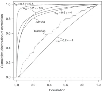
Realized spatial correlations in the simulations The simulations should cover a wide range of realistic levels of spatial correlation. The migration gene example rep-resents a case of strong correlation over the landscape (r 0.75 on average between a sampled position and its closest neighbour, average r 0.36 over the landscape). The
Loa loa prevalence example represents a case of stronger
correlation among such neighbours and more moderate autocorrelation overall (r 0.90 and r 0.13, respectively). Such autocorrelation is large enough to substantially impact the performance of partial Mantel tests of fixed effects (Guillot and Rousset 2013). Our simulation study covers a wider set of autocorrelation situations, as shown in Fig. 1. Bootstrap estimation of LR bias
For the bootstrap estimation of the LR bias, for each sample analyzed, 100 new samples are simulated under the null hypothesis, with estimated parameters under the null model, and with the same spatial locations as the original sample.
Figure 1. Cumulative distributions of spatial correlations of random effects for the different simulation conditions.
Effects of bootstrap correction
To illustrate the effect of the bootstrap correction, we considered bad-looking Poisson and binomial cases from the Tables. We further reduced the samples sizes, and per-formed PQL/L analyses, to accentuate small sample bias (with actually limited effect). The results are shown in Fig. 2 and confirms the effectiveness of the correction. The Gaussian case is illustrated in the next section.
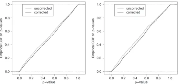
Ad hoc sampling designs and glmmPQL performance Simulations based on the migration gene study design exhibit a strong bias of the likelihood ratio test, as expected from such small samples. This case was used to check the efficiency of the bootstrap (with only 100 replicates) in cor-recting such a bias (Fig. 3 left).
For LMMs, the data sets can also be analyzed using the nlm procedure in R through a syntactic trick as described in Dormann et al. (2007, Appendix). However, this de facto constrains the analysis to models without residual error; the results are otherwise similar to those of the ML method (see Supplementary material Appendix G for details).
In simulations based on the onchorcerciasis study design, the likelihood ratio tests based on either ML or PQL/L exhibited little bias, while analyses based on glmmPQL and the same syntactic trick are strongly anticonservative (Fig. 3 right). These comparisons are based on the t-test in glmmPQL, as this procedure did not provide likelihood val-ues. Supplementary material Appendix G also presents the distributions of estimates by the different methods for all approximation, the pn(h) approximation for likelihood may
be inaccurately large for large l, and the second-order Laplace approximation even more so. For example, consider binary data in 6 locations, 5 ‘positive’ and one ‘negative’, for spatially independent random effects with linear predic-tor a ui (i 1,…,6). The log-likelihood (directly com-puted by numerical integration) is maximized for a ≈ 2, l ≈ 1.4; h-likelihood is maximized for a ≈ 1.7, l ≈ 0; pn(h)
for a ≈ 11.9, l ≈ exp(7.7), and the second-order approxi-mation appears to increase indefinitely, linearly with log(l) for a ≈ 0.
Although the joint estimates actually depend on the distinct objective functions used to estimate b and l, this example predicts the observed trends. The inaccuracies of the Laplace approximations lead to a high frequency of ML fits diverging to very large l values, often with no inferred spatial correlation, and to very inaccurate LR statistics. The PQL/L fits were comparatively much bet-ter behaved (Table 2). These problems may largely disap-pear in practice as soon as soon as two draws are made in each spatial location (Fig. F1 in Supplementary material Appendix F). The ML fits may still be useful under some conditions, as the distributions of p-values for samples that did not exhibit such a divergence were uniform. Likewise, the distribution was uniform if l estimates were constrained as 5 (Table 1). However, this con-straint expectedly raises other problems; for example if the true l 100 (with other parameters as in the fourth row of the table), the test of fixed effects appears conser-vative, the mean likelihood ratio chi-square statistic being 0.66.
Table 1. Performance of likelihood ratio tests. In each case, the table shows the proportion of significant tests at the conventional 0.05 and 0.01 levels, and the average value LR of the likelihood ratio chi-square statistic. For l, ‘low’ and ‘high’ values are respectively 0.1 and 2.5, except for the Poisson case where they are 0.06 and 0.763 (see main text). For binary samples, the l estimates were constrained below 5 (see main text).
Gaussian Poisson Binomial Binary (lˆ 5)
ssp n l 0.05 0.01 LR 0.05 0.01 LR 0.05 0.01 LR 0.05 0.01 LR 0.2 0.5 low 0.072 0.019 1.161 0.051 0.007 1.05 0.054 0.008 1.062 0.052 0.011 0.995 – – high 0.074 0.022 1.241 0.065 0.018 1.172 0.072 0.011 1.228 0.052 0.013 1.066 – 4 low 0.078 0.017 1.195 0.051 0.013 1.044 0.052 0.011 0.973 0.058 0.016 1.025 – – high 0.059 0.013 1.138 0.048 0.01 0.984 0.041 0.008 0.952 0.055 0.013 1.009 0.6 0.5 low 0.073 0.018 1.182 0.056 0.011 1.079 0.049 0.015 1.014 0.06 0.016 1.045 – – high 0.069 0.018 1.15 0.074 0.015 1.179 0.053 0.009 1.098 0.044 0.011 0.955 – 4 low 0.077 0.019 1.22 0.039 0.01 0.949 0.047 0.006 0.996 0.057 0.017 1.037 – – high 0.091 0.026 1.377 0.048 0.014 1.042 0.043 0.006 0.948 0.051 0.01 1.016
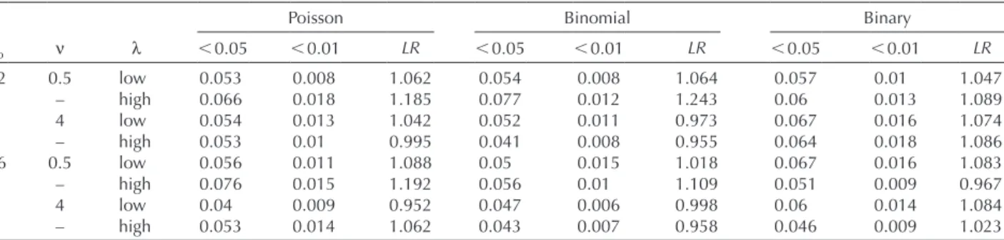
Table 2. Performance of PQL/L likelihood ratio tests. See Table 1 legend for details, except that l estimates were not constrained below 5 for binary samples. The samples analyzed are exactly the same in both tables.
Poisson Binomial Binary
ssp n l 0.05 0.01 LR 0.05 0.01 LR 0.05 0.01 LR 0.2 0.5 low 0.053 0.008 1.062 0.054 0.008 1.064 0.057 0.01 1.047 – – high 0.066 0.018 1.185 0.077 0.012 1.243 0.06 0.013 1.089 – 4 low 0.054 0.013 1.042 0.052 0.011 0.973 0.067 0.016 1.074 – – high 0.053 0.01 0.995 0.041 0.008 0.955 0.064 0.018 1.086 0.6 0.5 low 0.056 0.011 1.088 0.05 0.015 1.018 0.067 0.016 1.083 – – high 0.076 0.015 1.192 0.056 0.01 1.109 0.051 0.009 0.967 – 4 low 0.04 0.009 0.952 0.047 0.006 0.998 0.06 0.014 1.084 – – high 0.053 0.014 1.062 0.043 0.007 0.958 0.046 0.009 1.023
The results confirm that some testing biases, leading to too narrow confidence intervals, are observed for small samples, in particular in the Gaussian case, in which case a bootstrap correction is recommended. This correction is of more general interest as it should be fast, and easy to perform with alternative software, in non-spatial models. Otherwise, the testing biases are much smaller than those that can be observed for partial Mantel tests. For example, for the design based on the onchocerciasis study, Guillot and Rousset (2013) found that the error rate of the latter is 27.5% at the nominal level 5%. The spaMM package therefore allows for more reliable inferences. Another approach, where standard R software for linear mixed models is applied by specifying a dummy random effect, may sometimes yield good results but has several draw-backs. In linear mixed models, ML fits using the lme pro-cedure effectively constrain the residual error to zero, and simulated data sets, highlighting further problems with
glmmPQL.
Discussion
In this work we have implemented and assessed methods for fitting GLMMs, for the poorly implemented case of spatial data. Our simulations confirm that these methods allow inferences of environmental and genetic effects in spatially correlated landscapes. Although we have focused here on inferences about fixed effects, the Supplementary material shows that the new procedures also provide better estimates of the spatial autocorrelation parameters (Supplementary material Appendix G, Fig. G1 and G2) and that glmmPQL may not provide useful estimates of the variance of the autocorrelated random effects.
Figure 3. Distributions of p-values for slope (b) estimates from simulations based on real sampling designs. Left: results of uncorrected and bootstrap-corrected likelihood ratio tests for data simulated according to the migration gene study design; right: results of ML and PQL methods for data simulated according to the onchocerciasis study design. In contrast to glmmPQL, PQL/L and ML result are barely distinguishable.
Figure 2. Effects of bootstrap correction. Left: same parameters as in Poisson case, sixth row in Table 1 and 2, but with only 20 sampled locations. Right: same parameters as in binomial case, second row in Table 1 and 2, but with only 20 sampled locations with 20 draws per location.
values for the full analysis, as well as by more or less ad hoc optimization of the code, but not up to the point where interactive analyses can be considered. Sparse matrix techniques have often been used to analyze large data sets, or more generally to speed up computations (e.g. the lme4 package, Bates et al. 2012). Autoregressive models (Methods) have also been considered for the same reason, but as the spatial correlation matrices considered in this work are not inherently sparse, the feasibility of sparse matrix approximations and their ultimate impact on statistical inference is not obvious.
For binary data, Laplace approximations have clear weaknesses, in particular overestimating the likelihood of high variance of random effects. What is usually the crudest approximation, penalized quasi-likelihood, was here better behaved, and should be used at least whenever divergence of l estimates is observed in ML fits. This may be sufficient for the simple inferences problems considered in this work, but not more generally. Other approxima-tions to marginal and conditional likelihoods, and algo-rithms to fit models, could be considered. In particular, Diggle et al. (2003) developed MCMC methods for fitting the spatial GLMMs considered in this study. These meth-ods might perform well by the present criteria when prop-erly used, but this may be difficult to assess insofar as they require substantial user intervention on each data set (Diggle and Ribeiro 2007, p. 175). More recently, Rue et al. (2009) developed integrated nested Laplace integration (INLA), which may give results similar to those used in this work (see Lee in discussion of Rue et al. 2009). Several other techniques are discussed in the litera-ture (reviewed by Demidenko 2004, McCulloch et al. 2008), for mixed models distinct from the present one, and distributions of p-values (or coverage of confidence intervals) are rarely considered, so it is again difficult to anticipate how well they would perform.
A prominent question in the recent literature is how to detect the effect of environmental features, rather than simply geographical distance, on genetic structure (landscape genetics, Guillot et al. 2009, Storfer et al. 2010), and similar questions arise in species distribution modelling (Algar et al. 2013). In a GLMM framework, assessing landscape features on gene flow or individual dispersal is equivalent to testing whether the correlation matrix of random effects is a function only of distance or of other effects. This can be tested by comparing restricted likelihood values for models with different structures of the correlation matrix, provided that effects of landscape fea-tures on correlations among allele frequencies in different locations can be related to correlations among underlying Gaussian random effects in a GLMM.
In summary, inference problems in spatially autocorre-lated landscapes can be addressed by fitting spatial general-ized linear mixed models. Spatial analyses are recommended even in cases when spatial autocorrelation appears non- significant because of insufficient power. However, software implementations have been limited in various respects, and this approach is often ignored in ecological and evolu-tionary studies. We have shown that valid inferences of fixed effects can be performed in small samples, using Laplace approximation or even penalized quasi-likelihood were also found to diverge in a large proportion of
simula-tions. Likewise, glmmPQL should not be used to analyze non-Gaussian spatial data, as it performs substantially worse than our implementation for spatial data. This may not be a problem with glmmPQL per se, which has been shown to perform more satisfactorily in other applications (Hamel et al. 2012), but may stem from the fact that it has to be used in a non-standard way, to our knowledge not recommended by its authors, for the analysis of spatial data.
The main approximations used in this work have already been checked and compared to previous proposals such as penalized quasi-likelihood or Markov-chain simulation methods, mainly in terms of bias and variance of estimators for various specifications of the fixed and random effects (Lee et al. 2006, pp. 190–192, Noh et al. 2006, Pinheiro and Chao 2006, Jang et al. 2007, Noh and Lee 2007, Lee and Lee 2012). With the exception of the PQL/L results for binary data, the simulation results can be seen as a check of well-established, though approximate, likelihood methods for GLMMs. However, there does not appear to be comparable simulations for spatially correlated models in the literature. Ignoring autocorrelation may have little effect on the bias of estimates of fixed effects but should result in underestimates of the variance and too narrow confidence intervals. Thus, our assessment of the properties of likelihood ratio tests is much more informative than simple assessment of bias of estimators.
Comparison of models with or without spatial correla-tions is feasible within the present framework, as the model with spatial correlation includes the model without spatial correlation as a limit case (when the spatial scale parameter r become very large). However, for inference of fixed effects, it appears better to always include spatial auto-correlation in the analysis, even if autoauto-correlation appears non-significant. In particular, a non significant autocorrela-tion can arise in a real data set because few localities are sampled, but this does not necessarily mean that the auto-correlation does not impact inference of fixed effects, because the statistical information about a fixed effect in this data set can decrease with increasing assumed level of autocorrelation. Such cases can be detected by comparing confidence intervals for fixed effect under (say) the fitted non-zero autocorrelation, and in a model without autocorrelation. However, the proper interval for fixed effects is not the one given by the first of these two compu-tations. Rather, it is given by the profile likelihood ratios, which are designed to take into account uncertainty in nuisance parameters.
We have considered the Matérn correlation model for a first implementation, using generic matrix methods applicable to any correlation matrix. A well-known issue for mixed models is that the computation time of fitting algorithms involving such matrix computations increases sharply with sample size, here with the number of sampled locations. For example, tests of the effect of climate variables on single-nucleotide polymorphisms in Arabidopsis thaliana took nearly 10 CPU hours on 2 GHz processors on average (52 tests) when a large data set of 948 locations (Hancock et al. 2011) was considered. This can probably be shortened by first analyzing subsets of the data to define good starting
Golub, G. H. and van Loan, C. F. 1996. Matrix computations, 3rd ed. – John Hopkins Univ. Press.
Guillot, G. and Rousset, F. 2013. Dismantling the Mantel tests. – Methods Ecol. Evol. 4: 336–344.
Guillot, G. et al. 2009. Statistical methods in spatial genetics. – Mol. Ecol. 18: 4734–4756.
Ha, I. D. et al. 2007. Model selection for multi-component frailty models. – Stat. Med. 26: 4790–4807.
Hamel, S. et al. 2012. Statistical evaluation of parameters estimating autocorrelation and individual heterogeneity in longitudinal studies. – Methods Ecol. Evol. 3: 731–742. Hancock, A. M. et al. 2011. Adaptation to climate across the
Arabidopsis thaliana genome. – Science 334: 83–86.
Hoeting, J. A. et al. 2006. Model selection for geostatistical models. – Ecol. Appl. 16: 87–98.
Jang, M. J. et al. 2007. A comparison of the hierarchical likelihood and Bayesian approaches to spatial epidemiological modelling. – Environmetrics 18: 809–821.
Keitt, T. H. et al. 2002. Accounting for spatial pattern when modeling organism–environment interactions. – Ecography 25: 616–625.
Konis, K. 2009. safeBinaryRegression: safe binary regression. – R package ver. 0.1-2.
Lee, W. and Lee, Y. 2012. Modifications of REML algorithm for HGLMs. – Stat. Comput. 22: 959–966.
Lee, Y. and Nelder, J. A. 1996. Hierarchical generalized linear models. – J. R. Stat. Soc. B 58: 619–678.
Lee, Y. and Nelder, J. A. 2001a. Hierarchical generalised linear models: a synthesis of generalised linear models, random- effect models and structured dispersions. – Biometrika 88: 987–1006.
Lee, Y. and Nelder, J. A. 2001b. Modelling and analysing correlated non-normal data. – Stat. Model. 1: 3–16.
Lee, Y. et al. 2006. Generalized linear models with random effects: unified analysis via H-likelihood. – Chapman and Hall. Legendre, P. and Fortin, M.-J. 2010. Comparison of the Mantel
test and alternative approaches for detecting complex multi-variate relationships in the spatial analysis of genetic data. – Mol. Ecol. Resour. 10: 831–844.
Lunn, D. J. et al. 2000. WinBUGS – a Bayesian modelling framework: concepts, structure, and extensibility. – Stat. Comput. 10: 325–337.
Madsen, K. et al. 2004. Methods for non-linear least squares problems. – Technical report, Informatics and Mathematical Modelling, Technical Univ. of Denmark.
Martellosio, F. 2012. The correlation structure of spatial auto-regressions. – Econ. Theory 28: 1373–1391.
McCullagh, P. and Nelder, J. A. 1989. Generalized linear models, 2nd ed. – Chapman and Hall.
McCulloch, C. E. et al. 2008. Generalized, linear, and mixed models, 2nd ed. – Wiley.
Minasny, B. and McBratney, A. B. 2005. The Matérn function as a general model for soil variograms. – Geoderma 128: 192–207. Molas, M. and Lesaffre, E. 2011. Hierarchical generalized linear
models: the R package HGLMMM. – J. Stat. Softw. 39: 1–20.
Mueller, J. C. et al. 2011. Identification of a gene associated with avian migratory behaviour. – Proc. R. Soc. B 278: 2848–2856.
Nocedal, J. and Wright, S. J. 1999. Numerical optimization. – Springer.
Noh, M. and Lee, Y. 2007. REML estimation for binary data in GLMMs. – J. Multivariate Anal. 98: 896–915.
Noh, M. et al. 2006. Multicomponent variance estimation for binary traits in family-based studies. – Genet. Epidemiol. 30: 37–47.
Oden, N. L. and Sokal, R. R. 1992. An investigation of three-matrix permutation tests. – J. Classification 9: 275–290.
approaches. A simple bootstrap method is recommended for Poisson and binomial data sampled in fewer than 20 loca-tions, and more generally for Gaussian data. The present work makes all these tasks more practical, and provides more reliable inferences of both fixed and random effect parame-ters than previously available ones (in particular, glmmPQL), which cannot be recommended in a spatial context.
Acknowledgements – This work was supported by an exploratory program (PEPS) ‘Comprendre les maladies émergentes et les épidémies’. We thank N. Yoccoz for helpful comments on the man-uscript, Y. Lee, L. Rönnegård, M. Alam, and M. Molas for dis-cussion of h-likelihood methods and software, A. Courtiol for stimulating discussion about other R packages, and J.-M. Marin for further discussion and help in tracking some references. Most computations were performed on the ISEM computing cluster platform. We thank R. Dernat for assistance in using this cluster.
References
Algar, A. C. et al. 2013. Niche incumbency, dispersal limitation and climate shape geographical distributions in a species- rich island adaptive radiation. – Global Ecol. Biogeogr. 22: 391–402.
Baayen, R. H. et al. 2008. Mixed-effects modeling with crossed random effects for subjects and items. – J. Mem. Lang. 59: 390–412.
Bartlett, M. S. 1937. Properties of sufficiency and statistical tests. – Proc. R. Soc. A 160: 268–282.
Bates, D. et al. 2012. lme4: linear mixed-effects models using S4 classes. – R package ver. 0.999999-0.
Bini, L. M. et al. 2009. Coefficient shifts in geographical ecology: an empirical evaluation of spatial and non-spatial regression. – Ecography 32: 193–204.
Bolker, B. M. et al. 2009. Generalized linear mixed models: a practical guide for ecology and evolution. – Trends Ecol. Evol. 24: 127–135.
Bradburd, G. S. et al. 2013. Disentangling the effects of geographic and ecological isolation on genetic differentiation. – Evolution. 67: 3258–3273.
Breslow, N. E. and Clayton, D. G. 1993. Approximate inference in generalized linear mixed models. – J. Am. Stat. Assoc. 88: 9–25.
Breslow, N. E. and Lin, X. 1995. Bias correction in generalised linear mixed models with a single component of dispersion. – Biometrika 82: 81–91.
Coull, B. A. and Agresti, A. 2000. Random effects modeling of multiple binomial responses using the multivariate binomial logit-normal distribution. – Biometrics 56: 73–80.
Cox, D. R. 2006. Principles of statistical inference. – Cambridge Univ. Press.
Davison, A. C. 2003. Statistical models. – Cambridge Univ. Press.
Demidenko, E. 2004. Mixed models: theory and applications. – Wiley.
Diggle, P. and Ribeiro, P. 2007. Model-based geostatistics. – Springer.
Diggle, P. J. et al. 2003. An introduction to model-based geostatistics. – In: Møller, J. (ed.), Spatial statistics and computational methods. Springer, pp. 43–86.
Diggle, P. J. et al. 2007. Spatial modelling and the prediction of Loa loa risk: decision making under uncertainty. – Ann. Trop. Med. Parasitol. 101: 499–509.
Dormann, C. F. et al. 2007. Methods to account for spatial autocorrelation in the analysis of species distributional data: a review. – Ecography 30: 609–628.
Rousset, F. 2002. Partial Mantel tests: reply to Castellano and Balletto. – Evolution 56: 1874–1875.
Rue, H. et al. 2009. Approximate Bayesian inference for latent Gaussian models by using integrated nested Laplace approximations (with Discussion). – J. R. Stat. Soc. B 71: 319–392.
Stein, M. L. 1999. Interpolation of spatial data: some theory for Kriging. – Springer.
Stopher, K. V. et al. 2012. Shared spatial effects on quantitative genetic parameters: accounting for spatial autocorrelation and home range overlap reduces estimates of heritability in wild red deer. – Evolution 66: 2411–2426.
Storfer, A. et al. 2010. Landscape genetics: where are we now? – Mol. Ecol. 19: 3496–3514.
Wall, M. M. 2004. A close look at the spatial structure implied by the CAR and SAR models. – J. Stat. Plan. Inference 121: 311–324.
Pinheiro, J. C. and Bates, D. M. 2000. Mixed-effects models in S and S-PLUS. – Springer.
Pinheiro, J. C. and Chao, E. C. 2006. Efficient Laplacian and adaptive Gaussian quadrature algorithms for multilevel generalized linear mixed models. – J. Comput. Graph. Stat. 15: 58–81.
Raufaste, N. and Rousset, F. 2001. Are partial Mantel tests adequate? – Evolution 55: 1703–1705.
Rayner, R. K. 1990. Bartlett’s correction and the boostrap in normal linear regression models. – Econ. Lett. 33: 255–258. Robertson, G. P. and Freckman, D. W. 1995. The spatial
distribu-tion of nematode trophic groups across a cultivated ecosystem. – Ecology 76: 1425–1432.
Rocke, D. M. 1989. Bootstrap Bartlett adjustment in seemingly unrelated regression. – J. Am. Stat. Assoc. 84: 598–601. Rönnegård, L. et al. 2010. hglm: a package for fitting hierarchical
generalized linear models. – R J. 2: 20–27.
Supplementary material (Appendix ECOG-00566 at www.oikosoffice.lu.se/appendix). Appendix A–G and R scripts.