Modeling 3D Spatially Distributed Water Fluxes in an Andisol under Banana Plants

HAL Id: hal-02758430

https://hal.inrae.fr/hal-02758430

Submitted on 4 Jun 2020

HAL is a multi-disciplinary open access

archive for the deposit and dissemination of

sci-entific research documents, whether they are

pub-lished or not. The documents may come from

L’archive ouverte pluridisciplinaire HAL, est

destinée au dépôt et à la diffusion de documents

scientifiques de niveau recherche, publiés ou non,

émanant des établissements d’enseignement et de

Modeling 3D Spatially Distributed Water Fluxes in an

Andisol under Banana Plants

Julie Sansoulet, Yves-Marie Cabidoche, Philippe Cattan, Stéphane Ruy, J.

Simunek

To cite this version:

Julie Sansoulet, Yves-Marie Cabidoche, Philippe Cattan, Stéphane Ruy, J. Simunek. Modeling 3D

Spatially Distributed Water Fluxes in an Andisol under Banana Plants. 13. World Water Congress,

International Water Resources Association (IWRA). ZAF., 2008, Montpellier, France. �hal-02758430�

“Modeling 3D Spatially Distributed Water Fluxes in an Andisol under Banana Plants”

Julie Sansoulet et alii

Presented at the 13

World Water Congress ; Montpellier (France), 2008 september 1

-4

http://www.iwra.org/congress/2008/

Registered in

Prodinra

, INRA Open Archive (archive ouverte des productions de l’INRA)

Modeling 3D Spatially Distributed Water Fluxes in an Andisol under Banana Plants

Julie Sansoulet,* Yves-Marie Cabidoche, Philippe Cattan, Stéphane Ruy, and Jirka Šim nek

ABSTRACT

Subsurface environments are often highly heterogeneous and infiltration water is often distributed unevenly due to aboveground interception and redistribution of rainfall by the plant canopy. These phenomena significantly affect groundwater recharge and nutrient leaching. Field experiments involving subsurface lysimeters and tensiometers were performed to quantify the spatial distribution of fluxes in an Andisol under a banana plant. Wick lysimeters were installed at a depth of 70 cm at several locations with respect to the banana stem to measure the spatial distribution of subsurface water fluxes. Collected experimental data were simulated using the 3D HYDRUS software package. Spatially distributed drainage fluxes were well reproduced with the numerical model. Due to the impact of stemflow, drainage volumes under the banana stem were up to six times higher than in the row downstream from the stem, as well as between rows, as these areas were sheltered from direct rainfall by the banana leaves and received only throughfall.

J. Sansoulet and Y.-M. Cabidoche, Institut National de la Recherche Agronomique, Unité Agropédoclimatique de la Zone Caraïbe, Domaine Duclos, 97170 Petit-Bourg, Guadeloupe, France;

P. Cattan, Centre International de Recherche Agronomique pour le Développement, Unité Systèmes de Culture Bananes, Plantains et Ananas, Station Neufchâteau, 97130 Capesterre Belle Eau, Guadeloupe, France;

S. Ruy, Institut National de la Recherche Agronomique, Unité Climat-Sol-Environnement, Domaine Saint-Paul, Site Agroparc, 84914 Avignon, France;

J. Šim nek, Dep. of Environmental Sciences, Univ. of California, Riverside, CA 92521. Received 13 Apr. 2007. *Corresponding author (juliesansoulet@yahoo.fr).

INTRODUCTION

Stemflow is an important hydro-ecological process in forested and agricultural ecosystems because it results in a spatially localized input of water into the soil at the foot of the plant stem and thus significantly influences groundwater recharge (Taniguchi et al., 1996). Due to their large leaves, banana crops exhibit a strong partitioning of rainfall, resulting in a high amount of stemflow (Bassette and Bussière, 2005). Moreover, banana plants are often locally and intensively fertilized at the foot of the plant stem with up to 400 kg N ha−1 yr−1 and 800 kg K ha−1 yr−1 (Godefroy and Dormoy, 1988). Stemflow is thus likely to remove large quantities of these nutrients from the root zone and leach them into the deeper subsurface.

Extensive literature has been produced about rainfall interception in forested ecosystems (Carlyle-Moses and Price, 1999) and about the spatial variability of subsurface drainage due to different types of irrigation (Young and Wallender, 2002) and plant evapotranspiration (Arya et al., 1975). Still, few studies have been performed to quantify the effect of stemflow on the spatial pattern of drainage and associated solute leaching (Sansoulet et al., 2007). Among the large number of well-established modeling programs, HYDRUS (Šim nek et al., 2006) was selected to simulate water transfers under banana plant because it allows application of the different boundary conditions required for this problem (e.g., stemflow, throughfall, free drainage, and seepage face), has a sophisticated graphical user interface that simplifies the design of complicated three-dimensional geometries of the transport domain, enables consideration of different soil layers and their inclination, considers root water uptake, distinguishes between soil evaporation and plant transpiration, and simulates also solute movement.

This study was an extensive field study undertaken to evaluate distributed subsurface water fluxes under banana plants and to use the collected data to evaluate and numerically simulate these distributed water fluxes using the HYDRUS software package. Hence, the study had several phases: (i) laboratory experiments to obtain soil hydraulic parameters characterizing the unsaturated hydraulic conductivity function, K(h), and the soil water retention curve, (h); (ii) field experiments to measure surface water fluxes (stemflow and throughfall) and subsurface pressure heads and drainage fluxes; and (iii) numerical modeling using the HYDRUS model to predict distributed water fluxes and compare them to the in situ drainage measurements.

MATERIALS AND METHODS

Field Experiments

In the French West Indies intensive banana cultivation on volcanic ash soils has been going on since the 1960s (Ndayiragije, 1996). These soils, particularly the Andisols (Soil Survey Staff, 1996), are well known to have a high infiltration capacity. From 15 June to 29 Nov. 2004 (168 d), field experiments with installed lysimeters and tensiometers were performed to quantify the spatial distribution of drainage fluxes in an Andisol after rainfall interception by banana plants. The experiments were performed at the CIRAD research facility in Guadeloupe (Basse Terre), French West Indies (16°09 N, 61°16 W, 250 m above sea level).

The experimental field was a small watershed of 6000 m2 with an average slope of 12%. Planting of the banana plants (1800 plants ha−1) took place on 2 Apr. 2003. An automated meteorological station measured global and net radiation, air temperature, relative humidity, and wind speed and direction were measured every 15 s and then averaged and stored for 5-min intervals.

Five experimental plots were instrumented in June 2003. The first site was upslope of the field where the A horizon was 10 cm thinner (due to tillage erosion), two were downslope of the field where the soil accumulated, and two were in the middle of the field. One of the plots, called the fully equipped plot, was isolated from the neighboring soil with a metal sheet and equipped with a runoff collector (Fig. 1) and a stemflow collector (installed at the stem of the banana plant). The collectors for drainage, runoff, and stemflow at this site were also equipped with pressure transducers that were linked to the Campbell CR10 datalogger. At the other four plots, soil solution samplers were weighed manually after each rainfall event.

Distributed drainage was measured using glass wick lysimeters. Wick samplers with a fiberglass wick that maintains a fixed tension are the most appropriate and cost-effective devices for collecting the leachate (Boll et al., 1992;

Rimmer et al., 1995; Vandervelde et al., 2005). A 45- by 45- by 5-cm steel plate container was first filled with soil from the B horizon. And installed 30 cm below the A horizon. The soil profile above the lysimeters, including the banana plants, surface litter, the A and the B horizon, was not disturbed. Each experimental site included four lysimeters that intercepted water at different positions relative to the stem (Fig. 1). Twenty lysimeters were installed overall. Two lysimeters were considered to be affected by stemflow. Lysimeter 1 was located directly below the stem, while Lysimeter 2 was located between 25 and 70 cm downslope from the stem. The third lysimeter (Lysimeter 3) was also located in the row of banana plants between 120 and 165 cm downstream from the stem under the leaves of a neighboring banana plant. This lysimeter was considered to be affected by throughfall and only to a lesser extent by stemflow. The last lysimeter (Lysimeter 4) was installed between two banana plants between rows, 95 cm away from the banana stems.

Fig. 1. Schematic representation of the flow domain in the banana plantation with indicated locations of Lysimeters 1 to 4, tensiometers, and the stemflow collector.

Bac de ruissellement -0.5 0 0.5 1 X (m) 2.5 3 3.5 4 4.5 5 5.5 6 6.5 Y (m ) 4 3 2 1

vers les bidons munis de capteurs de pression

Lysimètres Faux-tronc du bananier Tensiomètres de surface Tensiomètres à 25 cm de profondeur Tensiomètres à 55 cm de profondeur Tuyaux Collerette Partiteur de stemflow Tôles

A series of tensiometers (SKT 850, SDEC, Reignac sur Indre, France), capable of measuring pressure heads between 0 and −99 kPa, were installed in multiple locations at each experimental site. In the fully equipped plot, tensiometers were installed at three depths (6, 25, and 55 cm) above the four lysimeters and around the banana plant (Fig. 1) and the time step for measurements was between 10 s (during rainfall) and 15 min (between rainfalls). At other sites, they were installed at 20-, 40-, and 60-cm depths near the banana stem and downslope from the stem in the row in four sets. Pressure heads were measured every 30 s, then averaged and stored for 15-min intervals. Tensiometers were connected to the same Campbell CR10 datalogger as the tipping bucket.

The topography of the fully equipped plot was measured using a Trimble 3300DR tacheometer (Trimble Geomatics, Dayton, OH). To evaluate the water balance, daily evapotranspiration (ET) before and after banana flowering was calculated during the 168-d experiment according to (i) Pellerin (1986), who expressed the potential evapotranspiration, ETP, as a function of the global radiation (i.e., ETP = 0.23 global radiation), and (ii) Monteith

(1965), who related the actual evaporation to its potential value using the crop coefficients k (i.e., ET = kETP).

Governing Flow Equation

Water flow was simulated using the HYDRUS model (Šim nek et al., 2006) to numerically solve the Richards equation (Richards, 1931) describing water movement in three-dimensional transport domains in variably saturated porous media. The governing water flow equation is written in a mixed form to ensure excellent mass balances of the numerical solution (Celia et al., 1990):

1

h

h

h

K

K

K

S

t

x

x

y

y

z

z

∂

∂

∂

∂

∂

∂

∂

=

+

+

−

−

∂

∂

∂

∂

∂

∂

∂

θ

where is the volumetric water content [L3 L−3], h is the pressure head [L], S is a sink term accounting for the root water uptake [T−1], z is the vertical coordinate [L], x and y are the horizontal coordinates [L], t is time [T], and K is the unsaturated hydraulic conductivity [L T−1]. The finite-element method is used in HYDRUS to numerically solve the governing partial differential equations.

Soil Hydraulic Properties

HYDRUS, similar to most models that simulate unsaturated water flow in soils, requires knowledge of two nonlinear functions: the unsaturated hydraulic conductivity function, K(h), and the soil water retention curve, (h). The relations K(h) and (h) are often parameterized using functions proposed by Mualem (1976) and van Genuchten (1980), which are referred to here as van Genuchten (VG) equations:

( )

(

)

1

h

h

θ − θ

θ

=

+ θ

+ α

( )

h

θ

= θ

n

m

=

1 −

1

(

)

( )

1

1

K h

=

K S

−

−

S

S

=

θ − θ

θ − θ

where r and s are the residual and saturated water contents [L3 L−3], respectively, is the inverse of the air-entry

value [L−1], n is the pore size distribution index, Ks is the saturated hydraulic conductivity [L T−1], Se is the relative

water saturation (dimensionless), and l is the tortuosity factor (dimensionless). What is an appropriate value of l is still the subject of debate. Earlier studies have set l equal to 0.5 as the best estimate proposed by Mualem (1976). To be able to account for the effects of soil structure, the soil saturated hydraulic conductivity was measured in the field directly using the double-ring infiltrometer method (Reynolds et al., 2002) applied to both A and B horizons (four replications). From the double ring experiment, we took the final steady-state infiltration flux from the inner ring and declared it to be Ks. The laboratory evaporation method (e.g., Wind, 1968; Mohrath et al., 1997; Šim nek et

al., 1998) was used to obtain the other soil hydraulic parameters (i.e., r, s, , and n).The soil hydraulic parameters

for both A and B horizons were then used for simulations with the HYDRUS model.

HYDRUS Simulations

Drainage fluxes calculated using the HYDRUS model were validated using the field drainage data between 25 Sept. and 9 Nov. 2004 (46 d) and statistically evaluated. The modeling period, which was shorter than the experimental period, was representative of the wet season during which the main drainage fluxes were recorded. We chose only 46 d to avoid long simulation times, as three-dimensional simulations are still very computationally demanding. The flow domain and finite element grid (Fig. 2) were defined so that boundary and initial conditions reproduced the in situ conditions. Water flow in a three-dimensional flow domain with four wick lysimeters (Fig. 2b) was first simulated using HYDRUS. Detailed microtopography measured in the field was used to reproduce the surface conditions. The transport domain was considered to be, on average, 0.7 m deep and the surface area was about 8 m2. Three different materials with different soil hydraulic properties were defined to account for two soil horizons (A and B) and the wicks.

Fig. 2. A schematic representation of the flow domain indicating (a) surface boundary conditions, (b) bottom boundary conditions, (c) pressure head initial conditions, and (d) tetrahedral finite element mesh.

(b) Banana stem Seepage Free drainage Lysimeter 4 -1.752 -1.666 -1.579 -1.493 -1.406 -1.319 -1.233 -1.146 -1.060 -0.973 -0.887 -0.800

Pressure Head - h[m], Min=-1.752, Max=-0.800

-1.752 -1.666 -1.579 -1.493 -1.406 -1.319 -1.233 -1.146 -1.060 -0.973 -0.887 -0.800

Pressure Head - h[m], Min=-1.752, Max=-0.800 (a) (c) (d) Stemflow Throughfall A horizon B horizon Lysimeter 1 Lysimeter 2 Lysimeter 3

Pressure heads measured with tensiometers on 25 Sept. 2004 were used as initial conditions (Fig. 2c). Stemflow and throughfall were used as atmospheric and time-variable flux boundary conditions, respectively, at the soil surface of the domain (Fig. 2a). Stemflow measured with the stemflow collector (Fig. 1) was applied on a small area around the plant stem to ensure the proper volume of infiltrating water. As Bassette (2005) has shown, for the banana plants at our experimental site stemflow increases the incident rainfall relative to the throughfall by 18 to 20 times.

The wicks were simulated using a modified seepage face boundary condition with a limiting pressure of −55 cm to account for the vertical part of the wick. The seepage face is a dynamic outflow boundary condition that changes dynamically according to the flow conditions in the system. HYDRUS assumed a uniform pressure head equal to −55 cm along the active part of the seepage face through which water seeped out of the wick, and then calculated water flux for this area. Free drainage was specified on the remaining part of the bottom of the transport domain (Fig. 2b). This boundary condition represents a unit hydraulic gradient. A zero flux boundary condition was applied to all vertical boundaries.

Transpiration was simulated using the sink term of Eq. [1]. Roots were assumed to be distributed uniformly both under the plant stem and between the rows in the upper 50 cm of the soil profile (A horizon) according to Lecompte et al. (2003). The water uptake was reduced from its optimal value due to the decrease in the calculated pressure heads according to the model of Feddes et al. (1978).

A finite element grid (Fig. 2d) was created using an automatic grid generator. The finite element grid consisted of a total of 33,090 nodes and 184,788 finite elements. Finally, the time discretization was defined using the initial time step of 0.0001 d and the minimum allowed time step of 0.00001 d.

Statistical Evaluation

The model performance was evaluated using all measured and simulated drainage data. The correspondence between observed and predicted soil water drainage fluxes was statistically evaluated using the coefficient of efficiency (E), defined by Nash and Sutcliffe (1970) as

(

)

(

)

observed

predicted

1

observed

mean

E

−

= −

−

RESULTS AND DISCUSSION

Estimation of Soil Physical and Hydraulic Properties

The physical and chemical properties of the Andisol (Table 1) were in the range expected for Andisols containing allophane (Quantin, 1994). Particularly relevant are the very low bulk density values, the high C content, and the large total porosity considering the large clay content of these soils.

Table 1. Physical properties of the Andisol: clay content, bulk density, organic C, and total porosity.

Horizon Clay† Bulk density Organic C Total porosity

% g cm−3 % m3 m−3

A 58.6 0.71 6.69 0.673

B 63.1 0.49 3.73 0.665

† Clay content was determined by quantitative recovery of clay after sonication and dispersion with Na+ -saturated resins and before H2O2 oxidation of organic matter.

Soil hydraulic parameters for the VG functions for different soil layers are presented in Table 2. Specifically, the Mualem pore size distribution model (Mualem, 1976; van Genuchten, 1980) was used to predict K(h) from retention curves determined from the evaporation experiments and the saturated hydraulic conductivity determined from the infiltration experiments. It should be noted that the wick could not limit the flow of water in the soil because its hydraulic conductivity is considerably higher than the hydraulic conductivity of either horizon for all pressure heads

Table 2. Effective soil hydraulic parameters† obtained using the Wind and double-ring infiltrometer methods (direct measurements). Material r s n Ks l ———— m3 m−3 ———— m−1 m d−1 A horizon 0.13 0.75 19.0 1.07 3 0.5 B horizon 0.11 0.75 23.3 1.05 1.06 0.5 Wick 0 0.63 0.06 3.61 280 0.5

† r and s, residual and saturated volumetric water contents; inverse of the air-entry value; n, pore size

distribution index; Ks, saturated hydraulic conductivity; l, tortuosity factor.

Experimental Results

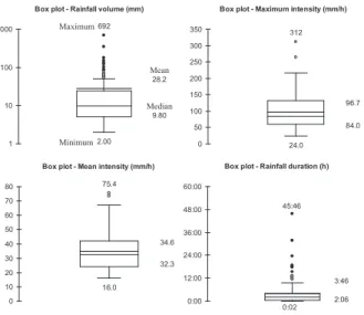
The annual rainfall (6568 mm) and average temperature (24.1°C) measured in 2004 were quite different from the average values of 3565 mm and 24.4°C collected from 1979 to 1999 by Météo France (2000). During the 168-d experiment, the cumulative rainfall was 4120 mm, with 141 rainfall events with volumes >2 mm. The characteristics of these events, given in terms of volume, intensity, and duration, are presented in Fig. 3. A mean rainfall had a volume of 28.2 mm, a maximum intensity of 96.7 mm h−1, an average intensity of 34.56 mm h−1, and a mean duration of 3 h 46 min, whereas a median rain had a lower volume (9.8 mm) and duration (2 h 6 min) and equivalent intensities. The largest rainfall, which had a volume of 692 mm, maximum intensity of 312 mm h−1, and maximum duration of 45 h 46 min, occurred at the end of the experimental period in November 2004 and was not representative of the other rainfall events.

Fig. 3. Box plots characterizing statistical properties of rainfall volume, rainfall duration, and maximum and mean rainfall intensities. Maximum and minimum values as well as first, second, third, and fourth quartiles and mean and median values are plotted.

Mean

Median

Box plot - Maximum intensity (mm/h)

312 24.0 96.7 84.0 0 50 100 150 200 250 300 350

Box plot - Mean intensity (mm/h)

75.4 16.0 34.6 32.3 0 10 20 30 40 50 60 70 80

Box plot - Rainfall duration (h)

0:00 12:00 24:00 36:00 48:00 60:00 3:46 2:06 45:46 0:02

Box plot - Rainfall volume (mm)

692 2.00 28.2 9.80 1 10 100 1000 Median Mean Maximum Minimum

Measured pressure heads below the plant foot and between the rows at three depths (6, 25, and 55 cm), as well as daily rainfalls, are represented in Fig. 4. Pressure heads recorded below the plant foot are, at all depths, on average about 21% higher than pressure heads recorded between the rows. This is mainly due to higher infiltration at the plant foot because of stemflow. Tensiometers installed closer to the soil surface reacted faster and to a greater extent than those at deeper depth. They were more strongly affected by climatic conditions (rain, evaporation, and transpiration).

Fig. 4. Mean pressure heads (calculated from five sets, CV = 17%) measured with tensiometers in the soil (top) at the foot of the plant stem (Lysimeter 2) and (bottom) between rows (Lysimeter 4). Precipitation rates are also shown in both figures.

Under the banana stem

-3.5 -3 -2.5 -2 -1.5 -1 -0.5 0 0 20 40 60 80 100 120 140 160 Time, d P re s s u re H e a d , m 0 50 100 150 R a in fa ll , m m

Between the rows

-3.5 -3 -2.5 -2 -1.5 -1 -0.5 0 0 20 40 60 80 100 120 140 160 Time, d P re s s u re H e a d , m 0 50 100 150 R a in fa ll , m m Rainfall 6 cm - Observed 25 cm - Observed 55 cm - Observed

HYDRUS Model Simulations and Mass Balance

The total rainfall during the 46-d modeling period was 1367 mm. Pressure heads illustrating the three-dimensional pattern of water flow during a rainfall event under the banana plant are shown in Fig. 5. This figure clearly shows that most of the water flow is concentrated around the stem of the banana tree, while reduced fluxes are apparent downstream from the stem in the row and between the rows.

Fig. 5. Pressure heads illustrating the three-dimensional water flow under the banana plant during a rainfall event (total rainfall = 65 mm).

a

b

c

Figure 5 shows the measured and simulated cumulative drainage fluxes from the four lysimeters vs. time. The mass balance error of the water flow simulation was <1%. Simulations showed that under heavy fluxes, such as those due to stemflow, the wicks reproduced the actual field drainage reasonably well. Mass transfers across the wick–soil interface are determined by differences in pressure heads between the wick and the soil. Under the driest conditions, which corresponded to the lower drainage volumes, pressure heads in the wick were higher than in the soil and the drainage flow stopped. When pressure heads at the bottom of the soil profile decreased below −0.55 m, the flow through the seepage face stopped.

Fig. 5. Measured and simulated cumulative fluxes from four lysimeters.

0 200 400 600 800 1000 1200 1400 0 10 20 30 40 Time, d C u m u la ti v e F lu x , m m 0 20 40 60 80 100 120 140 160 180 200 R a in fa ll , m m Rainfall Lysimeter 1 - observed Lysimeter 2 - observed Lysimeter 3 - observed Lysimeter 4 - observed Lysimeter 1 - simulated Lysimeter 2 - simulated Lysimeter 3 - simulated Lysimeter 4 - simulated 103 113 123 133 143

Both measurements and calculations showed relatively fast responses of drainage fluxes in Lysimeters 1 and 2 to rainfall events. Although the overall correspondence between measured and calculated fluxes is very high, there are some distinct differences. While measured drainage in Lysimeters 1 and 2 continued, although at very small rates, even during time periods without rainfall, calculated drainage started and ended rather abruptly and there were long time periods of no calculated drainage. This is because of the type of boundary conditions that were used by the model to represent lysimeters. Lysimeters were modeled using the seepage face boundary condition, which is active when pressure heads exceed the limiting value (−55 cm) and becomes inactive when pressure heads drop below this value.

The numerical model using the measured hydraulic parameters obtained from laboratory and in situ experiments reproduced the general trends of distributed drainage measured using lysimeters under the banana plant fairly well (Fig. 9). Indeed, the comparison of model simulations with field experimental results confirmed that simulated and measured data were quite similar. The model performance was evaluated by comparing the observed and predicted cumulative drainage in Lysimeters 1, 2, 3, and 4 (Fig. 9), as well as observed and predicted pressure heads (Fig. 10) at different soil depths and locations. The coefficient of efficiency (E) ranged from 0.62 to 0.76. The model slightly overestimated fluxes downslope from the plant stem, however. This can be explained by possibly higher root water uptake from deeper soil layers than anticipated. Simulations and collected drained volumes, as well as measured soil pressure heads, demonstrated that the flow under the banana tree was entirely dominated by stemflow and its redistribution in the soil profile. Stemflow infiltrated directly along the plant stem, but part of it was redirected downstream from the stem due to the slope. The drained volumes under the banana stem were six times higher than those downstream from the stem in the row and between the rows since these zones were sheltered by the banana leaves and received essentially only throughfall. Simulations showed that under heavy fluxes, such as those due to stemflow, the wicks reproduced the actual field drainage reasonably well.

CONCLUSIONS

Using experimental and calculated drained volumes, as well as soil pressure head data, we attributed drainage fluxes under the banana stem or immediately downstream from the stem almost exclusively to the stemflow. The drained volumes under the banana stem were six times higher than 1.2 m downstream from the stem in the row and between

the rows, since both these zones were sheltered by the banana leaves and received essentially only throughfall. Simulations showed that under heavy fluxes, such as those due to stemflow, the wicks reproduced the actual field drainage reasonably well. Under smaller surface fluxes (e.g., throughfall), measured water fluxes with lysimeters were, on average, 50% underestimated compared with simulated water fluxes without lysimeters.

The spatially distributed water fluxes under the banana plant also considerably influence solute transport. Our results, i.e., a concentrated water flow around the plant stem, bring into question the common practice of applying fertilizers and pesticides at the foot of the plant. Under these conditions, the abundant stemflow may rapidly leach the soluble nutrients or pesticides from the root zone into deeper horizons, and eventually into the groundwater. We therefore recommend that additional research be conducted to evaluate how our results can be interpreted in the context of a locally and intensively fertilized banana plantation. Such research could provide better guidelines for fertilization practices that would better protect subsurface water resources.

REFERENCES

Arya, L.M., G.R. Blake, and D.A. Farrell. 1975. A field study of soil water depletion patterns in presence of growing soybean roots: II. Effect of plant growth on soil water pressure and water loss patterns. Soil Sci. Soc. Am. J. 39:433–436.

Bassette, C., and F. Bussière. 2005. 3-D modelling of the banana architecture for simulation of rainfall interception parameters. Agric. For. Meteorol. 129:95–100.

Boll, J., T.S. Steenhuis, and J.S. Selker. 1992. Fiberglass wicks for sampling of water and solutes in the vadose zone. Soil Sci. Soc. Am. J. 56:701–707.

Carlyle-Moses, D.E., and A.G. Price. 1999. An evaluation of the Gash interception model in a northern hardwood stand. J. Hydrol. 214:103–110.

Celia, M.A., E.T. Bouloutas, and R.L. Zarba. 1990. A general mass-conservative numerical solution for the unsaturated flow equation. Water Resour. Res. 26:1483–1496.

Feddes, R.A., P.J. Kowalik, and H. Zaradny. 1978. Simulation of field water use and crop yield. John Wiley & Sons, New York.

Godefroy, J., and M. Dormoy. 1988. Mineral fertilizer element dynamics in the “soi–banana–climate” complex. Application to the programming of fertilization: III. The case of Andosols. Fruits 43:263–267.

Lecompte, F., H. Ozier-Lafontaine, and L. Pagès. 2003. An analysis of growth rates and directions of growth of primary roots of field-grown banana trees in an Andisol at three levels of soil compaction. Agronomie 23:209– 218.

Météo France. 2000. Bulletin climatologique annuel. Service Régional de la Guadeloupe, France.

Mohrath, D., L. Bruckler, P. Bertuzzi, J.C. Gaudu, and M. Bourlet. 1997. Error analysis of an evaporation method for determining hydrodynamic properties in unsaturated soil. Soil Sci. Soc. Am. J. 61:725–735.

Monteith, J.L. 1965. Evaporation and environment. p. 205–234. In G.E. Fogg (ed.) The state and movement of water in living organisms. Symp. Soc. Exp. Biol., 19th, Swansea. 8–12 Sept. 1964. Vol. 19. Cambridge Univ. Press, Cambridge, UK.

Mualem, Y. 1976. A new model for predicting the hydraulic conductivity of unsaturated porous media. Water Resour. Res. 12:513–522.

Nash, J.E., and J.V. Sutcliffe. 1970. River flow forecasting through conceptual models: Part I. A discussion of principles. J. Hydrol. 10:282–290.

Ndayiragije, S. 1996. Caractérisation d’une séquence d’altération de sols dérivés de matériaux pyroclastiques sous climat tropical humide des Antilles (Guadeloupe). Ph.D. diss. Université Catholique de Louvain, Louvain, Belgium.

Pellerin, S. 1986. Etude d’une série chronologique de rendements de canne à sucre obtenus en Guadeloupe à partir d’un modèle de simulation du bilan hydrique. Agronomie 6:91–98.

Quantin, P. 1994. The Andosols. p. 848–859. In Trans World Congr. of Soil Sci., 15th, Acapulco, Mexico. 10– 16 July 1994. Vol. 6a.

Reynolds, W.D., D.E. Elrick, and E.G. Youngs. 2002. Single-ring and double- or concentric-ring infiltrometers. p. 821–826. In J.H. Dane and G.C. Topp (ed.) Methods of soil analysis: Part 4. Physical methods. SSSA Book Ser. 5. SSSA, Madison, WI.

Richards, L.A. 1931. Capillary conduction of liquids through porous media. Physics 1:318–333.

Rimmer, A., T.S. Steenhuis, and J.S. Selker. 1995. One-dimensional model to evaluate the performance of wick samplers in soils. Soil Sci. Soc. Am. J. 59:88–92.

Sansoulet, J., Y.M. Cabidoche, and P. Cattan. 2007. Adsorption and transport of nitrate and potassium in an Andosol under banana (Guadeloupe, French West Indies). Eur. J. Soil Sci. 58:478–489.

Šim nek, J., M.Th. van Genuchten, and M. Šejna. 2006. The HYDRUS software package for simulating two- and three-dimensional movement of water, heat, and multiple solutes in variably saturated media. Technical manual, Version 1.0. PC Progress, Prague, Czech Republic.

Šim nek, J., O. Wendroth, and M.Th. van Genuchten. 1998. A parameter estimation analysis of the evaporation method for determining soil hydraulic properties. Soil Sci. Soc. Am. J. 62:894–905.

Soil Survey Staff. 1996. Keys to Soil Taxonomy. 7th ed. U.S. Gov. Print. Office, Washington, DC.

Sommer, R., H. Folster, K. Vielhauer, E.J.M. Carvalho, and P.L.G. Vlek. 2003. Deep soil water dynamics and depletion by secondary vegetation in the eastern Amazon. Soil Sci. Soc. Am. J. 67:1672–1686.

Taniguchi, M., M. Tsujimura, and T. Tanaka. 1996. Significance of stemflow in groundwater recharge: 1. Evaluation of the stemflow contribution to recharge using a mass balance approach. Hydrol. Proc. 10:71–80. Vandervelde, M., S.R. Green, G.W. Gee, M. Vanclooster, and B.E. Clothier. 2005. Evaluation of drainage from passive suction and nonsuction flux meters in a volcanic clay soil under tropical conditions. Vadose Zone J. 4:1201–1209.

van Genuchten, M.Th. 1980. A closed form equation for predicting the hydraulic conductivity of unsaturated soils. Soil Sci. Soc. Am. J. 44:892–898.

Wind, G.P. 1968. Capillary conductivity data estimated by a simple method. p. 181–191. In P.P.E. Rijtema and H. Wassink (ed.) Water in the unsaturated zone. Proc. Wageningen Symp., the Netherlands. 19–25 June 1966. Vol. 1. Publ. 82. Int. Assoc. Scientific Hydrol., Gentbrugge, Belgium.

Young, C.A., and W.W. Wallender. 2002. Spatially distributed irrigation hydrology: Water balance. Trans. ASAE 45:609–618.