Efficient Monitoring of Loose-Ordering Properties for SystemC/TLM

HAL Id: hal-01243246

https://hal.univ-grenoble-alpes.fr/hal-01243246

Submitted on 14 Dec 2015

HAL is a multi-disciplinary open access

archive for the deposit and dissemination of

sci-entific research documents, whether they are

pub-lished or not. The documents may come from

L’archive ouverte pluridisciplinaire HAL, est

destinée au dépôt et à la diffusion de documents

scientifiques de niveau recherche, publiés ou non,

émanant des établissements d’enseignement et de

Efficient Monitoring of Loose-Ordering Properties for

SystemC/TLM

Yuliia Romenska, Florence Maraninchi

To cite this version:

Yuliia Romenska, Florence Maraninchi. Efficient Monitoring of Loose-Ordering Properties for

Sys-temC/TLM. Design, Automation, and Test in Europe (DATE), Mar 2016, Dresden, Germany.

�hal-01243246�

Efficient Monitoring of Loose-Ordering

Properties for SystemC/TLM

Yuliia Romenska and Florence Maraninchi

Univ. Grenoble Alpes, VERIMAG, F-38000 Grenoble, France

CNRS, VERIMAG, F-38000 Grenoble, France

December 14, 2015

Abstract

SystemC Transaction-level modeling (TLM) provides high-level component-based models for SoCs, for which assertion-Based-Verification (ABV) allows property checking early in the design cycle. We introduce the notion of loose-ordering to specify when components interact with each other and we propose a set of patterns to capture this notion in assertions.

This new notion can already be expressed in languages like PSL, for which there exist tools to generate ABV monitors. But the definition of dedicated patterns makes it easier to write the properties. Moreover we define a direct translation of these patterns into SystemC monitors, and we show that it avoids the combinatorial explosion that would occur during a prior translation into PSL.

1

Introduction

SystemC-based Transaction-level modeling (TLM) [9] has been very successful in providing high-level executable component-based models for systems-on-chip (SoCs). The rationale has been to raise the level of abstraction by removing details of lower models like RTL models, especially on timing aspects. The notion of loose-timing is very interesting in that perspective. Exact delays in SystemC models (e.g., wait(100, SC_NS);) have been identified as a source of over-constraints and spurious synchronizations in models. The Loose-timing principle allows to write wait (90, 110, SC_NS), to specify a non-deterministic delay.

∗_{This work has been partially supported by the European CATRENE project CA703 and}

by the LabEx PERSYVAL-Lab (ANR–11-LABX-0025).

Introducing Loose-Ordering In this paper, we identify another source of over-constraints. Typically, when a component needs several input data (e.g., the address of an image, the size of it, etc.) before one of the functions it provides (e.g., some transformation of the image) can be started, the order in which the input data elements are provided is usually irrelevant. The same is true for data and control outputs. Any specification in which the order is imposed is over-constrained.

This type of property can already be expressed in languages like the Property Specification Language (PSL) [7, 3] (in the whole paper, PSL stands for PSL 1.1). But even simple loose-ordering properties require complex formulas, hence dedicated constructs are helpful.

Efficient Monitoring for Loose-ordering properties The first idea is to translate automatically our new properties into PSL, for which there exists monitor generation techniques. However, we will show that this produces complex formulas. Then, even the efficient techniques for exploiting such logics (e.g., the automatic modular generation of monitors described in [11, 14]) cannot do better than producing complex monitors from the obtained complex formulas.

The contributions are (i) a new notion called loose-ordering, allowing to remove the sources of over-constraints due to the order of interactions between components in a TL model; (ii) a set of patterns to capture these properties; (iii) a translation into PSL, for comparison purposes; (iv) a direct translation into efficient SystemC monitors.

2

Background and Related Work: Testing and

Monitoring Hardware Designs

Figure 1 illustrates the general method for testing a design-under-verification (DUV), as presented in the Universal Verification Methodology (UVM) [4], SystemC/SCV [13], eRM [10, 1], SVM [12], etc. A stimuli generator is in charge of producing inputs for the DUV; an assertion checker is in charge of deciding whether the test passes. An additional element of the method is a tool capable of evaluating the coverage of the design obtained with a set of stimuli.

Stimuli

Generator AssertionsChecker inputs outputs

Coverage Improver DUV

(Design Under Verification)

Figure 1: The verification framework

Assertions can be expressed with languages providing temporal logic con-structs, i.e., ways of expressing what happens on a (finite or infinite) sequence of states. For instance PSL is built on the Linear Temporal Logic (LTL). The

general method can be applied at various levels of abstraction. At the RT level, specifications are synchronous, and all the properties of the DUV can be expressed by specifying what happens on a unique discrete time scale.For TL models, the semantics of specification languages has to be adapted [14]. The idea is to recover the notion of a unique discrete scale on which to interpret the temporal logic constructs, by using the sequence of events instead of a unique clock.

In this paper, we focus on TL models. We follow the ideas of [14] for generating efficient monitors from our patterns, in a modular way. We compare with PSL, often used in assertion-based verification. Logics like the duration calculus or its discrete version [8], which offer a “chop” operator to express sequences, could be more appropriate for the expression of our patterns, but they are not usual in the domain.

3

The Case-Study

Our case-study is an access-control device based on face recognition analysis. A virtual prototype of the system has been implemented using standardized SystemC/TLM (see Fig. 2).

GPIO SEN IPU LCDC INTC

TMR1 MEM LOCK TMR2 CPU Bus

Figure 2: The TLM platform of the device. It includes: a component to handle buttons (GPIO); an image sensor (SEN); an image processing unit (IPU); an LCD controller (LCDC); an interrupt controller (INTC); two timers (TMR1, TMR2); the system’s memory (MEM); a door lock actuator (LOCK); a bus (Bus); and a central processing unit (CPU); the embedded software controls the face recognition process.

We focus on the Image Processing Unit (IPU), which performs face recognition. It contains read/write registers to configure the component; after termination of recognition, the IPU sends an interrupt through its channel irq. Its input/output interface is defined as follows: an input of the IPU is any action of the other components that affects the IPU (e.g. set_X standing for ’write’ operation on the register X, start launching recognition); output is any activity performed by the IPU that affects other components (e.g. read_img standing for ’read image’, set_irq for the interrupt signal). The specification of interactions is: (i) the input start must be preceded by at least one occurrence of each of the inputs set_X for all registers X, but the order does not matter (see Example 2 below); (ii) after face recognition has been requested (input start), the IPU reads images

Grammar Rule Constraints a range α(R) = {n} ⊆ I ∪ O R = n[u,v] u, v ∈ N a fragment i 6= j =⇒ α(Ri) ∩ α(Rj) = ∅ F = ({R1, . . . , Rn}, ]) ] ∈ {∧, ∨} a loose-ordering i 6= j =⇒ α(Fi) ∩ α(Fj) = ∅ L = F1< · · · < Fq P = L α(P) ⊆ I ∪ O Q = L α(Q) ⊆ O

an antecedent requirement α(P) ∩ {i} = ∅

A = (P << i, b) i ∈ I, b ∈ B

a timed implication constraint

t ∈ N T = (P ⇒ Q, t)

Figure 3: Abstract grammar and constraints for well-formed formulas

from the gallery (i.e., repeats the output read_img several times in a row) and then sends an interrupt (i.e., produces the output set_irq, see Example 3).

4

Specification Patterns for Loose-Orderings

We generalize the case-study properties with two patterns for: antecedent requirements and timed implication constraints. Both patterns are written on the vocabulary of the input/output interface (I, O) of the component. The syntax is given by the abstract grammar shown in Fig. 3. The right column of the table is the set of additional constraints defining well-formed formulas of this grammar. They are expressed using α, which denotes the set of interface names (inputs or outputs) that appear in the formula. The constraints mainly state that we should not reuse the same interface names in two ranges, or fragments, of the same property. All well-formed formulas are interpreted on sequences where only the names of the root pattern appear; only one name at a time can occur due to asynchrony of considered models. The notion of time used in the timed implication constraint will be mapped directly to the simulation time of the SystemC simulation kernel.

Definition 1: Range — A range R = n[u,v] denotes any sequence of k occurrences of n, n ∈ I ∪ O and k ∈ [u, v].

Definition 2: Fragment — A fragment F = ({R1, . . . , Rn}, ]), ] ∈ {∧, ∨} is

made of sequences s1, ...sn matching the corresponding ranges. If ] = ∧ then all

these sis should appear, concatenated in any order; if ] = ∨, at least one of these

sis should appear, and possibly several of them, concatenated in any order.

Definition 3: Loose-Ordering — A loose-ordering L = F1< · · · < Fq is

made of sequences s1, ...sn matching the corresponding fragments. All the sis

because the order in fragments is free.

Example 1: Loose-Ordering — Consider the loose-ordering ` = n[2,8]1 <

({n2, n3}, ∨). It defines sequences such that: first we have several n1 in a row

(the number of occurrences of n1is in [2, 8]); then we have either n2or n3, or

both in any order.

Definition 4: Antecedent requirement — An antecedent requirement A = (P << i, b), b ∈ B, means that i can occur only if P has been observed before. When b is true the condition has to be repeated: each occurrence of i should be preceded by its “own” occurrence of P, i.e. an occurrence that happened since the last i. When b is false one occurrence of P is enough to validate all the further occurrences of i.

Example 2: Non-repeated requirement with a conjunction — Before starting face recognition the environment of the IPU has to provide values of the image to be analyzed, the address of the image gallery, and the size of the gallery:

(({set_imgAddr, set_glAddr, set_glSize}, ∧) << start, false).

Definition 5: Timed implication constraint — A timed implication constraint T = (P ⇒ Q, t) means that, whenever P has been observed, Q should occur, and should have finished before t time units have elapsed since the end of P. This pattern is implicitly of the “repeated” kind: when P has been observed, Q should occur, and if a new occurrence of P is observed, a new occurrence of Q should occur.

Example 3: Timed implication constraint — If the recognition starts, the IPU reads images from the gallery (i.e., produces several times the output read_img) and sends an interrupt (the output set_irq). All outputs must be produced during some time interval T, which models the duration taken by the face recognition: (start ⇒ read_img[100,60000]< set_irq, T )

5

Translation into PSL

The translation has been validated with the SPOT tool [2] which translates LTL or PSL formulas into Büchi automata.

Dealing with Ranges Temporal logics lack counting facilities. One way to encode ranges is to use a big disjunction of nested next operators encoding all sequences defined by ranges. This encoding is explosive. The alternative approach to encode a range (e.g. n[1,2]_{) is to treat sequences of consecutive occurrences}

of a range’s name (e.g. n and nn) as new elements (e.g. n1 _{and n}2_{). The new}

vocabulary of n[1,2] _{is α = {n}1_{, n}2_{} (instead of α = {n}). Implementation of this}

approach includes a lexical analyzer to define new elements.

Encoding of Antecedent Requirements The encoding of A = (P << i, true) is a big conjunction of the expressions: Asynch –V always( not(nx∧ ny))

for all nx, ny ∈ α(A); MaxOne – before the occurrence of i each name of

P can occur at most once, V always(nx → next(not nx until! i)) for all

nx ∈ α(P); Range – before the occurrence of i at most one name per range

Rk of the loose-ordering P can occur,V always(nxk → (not n y

k until! i)) for all

nx_k, ny_k∈ α(Rk), for all ranges Rks; Order – if any of the names of the fragment

Fk occurs, all names of the preceding fragment Fk−1 have lost their turn,

V always(nx → (not(my) until! i)) for all nx ∈ α(Fk), for all my ∈ α(Fk−1);

BeforeI – the name i can occur only after P has been observed,V(not(i) until! nx)

for all nx∈ α(P); AfterI – the loose-ordering P should be observed before each

occurrence of the name i (i.e., i plays the role of a reset point),V always(i → next(W(not(i) until! nx

k))) whereW stands for all nxk∈ α(Rk), for all the ranges

Rks of P and for all fragments F s of P with ] = ∨.

Encoding of Timed Implication Constraints We can translate G = (P ⇒ Q, t) into PSL applying the encoding proposed above. To do that we need to (i) “concatenate” P and Q giving F₁p< · · · < F_kp< F₁q < · · · < F_{`</sub>q, (ii) consider the end of Q (i.e., the fragment F<sub>`}q) as the reset point.

6

Modular Monitors in SystemC

All the monitors are expressed as synchronous parallel compositions of elemen-tary recognizers for ranges (Fig. 5). The proposed constructions have been programmed in Lustre [6]; it allows to check their correctness with respect to the intuitive semantics given in section 4 using automatic testing tools.

The Recognition Context A recognizer for a range works in a recognition context, depending on where the range appears in the syntax tree of A or G. Consider for example the property of Figure 4. While recognizing n[2,8]₃ : (i) n1

and n2 are forbidden, since they are supposed to have happened before, the

set of such names is denoted as B; (ii) n4is forbidden unless n3 has occurred

at least twice (notice that n4can occur both before and after the range n [2,8] 3 ,

because it belongs to the same parent fragment F2), this set of names is denoted

as C; (iii) n5 is forbidden until n3 has been observed at least twice, in which

case it stops the recognition of the range n[2,8]₃ (and starts the recognition of the appropriate range), the appropriate set of names is Ac; (iii) i is forbidden

since it must occur after n3 and it may not act as a stopping condition, the set

of names is Af. Moreover, the recognizer for a range depends on whether its

parent fragment has a conjunctive (∧) or disjunctive (∨) semantics. Therefor, the context for a range recognizer is a tuple (B, C, Ac, Af, s), where s ∈ {∧, ∨}

stands for the semantics of the parent fragment.

Elementary Recognizers for Ranges The elementary recognizer for a range with context is shown in Figure 5. It is started with the input start, termination is signaled by the outputs ok or nok. In s0 it is idle and waits to be started; s5

is the error state; in s1it is started and waits for the first occurrence of its name

n; in s3 it is counting the occurrences with cpt; in s2 it is started and waits

for the first occurrence of its name n, another range of the same fragment has started; in s4 the minimum number of occurrences of n have been recognized,

and another range of the same fragment has started.

Recognizers for Fragments The recognizer for a fragment F = ({R1, . . . , Rn}, ]) with ] ∈ {∧, ∨} is the synchronous parallel composition of

the recognizers for the Ris. At any time these recognizers can be in one of the

following global states: (i) all are idle (state s0); (ii) all are waiting in state s1;

(iii) exactly one recognizer is counting (state s3) and all others are either still

waiting for their names to come (state s2) or have already recognized their ranges

(state s4). If the semantics s inherited from the parent fragment F is disjunctive

(i.e. s=∨), each recognizer can be stopped before it has even started counting, provided that at least one of the other ranges of F has started recognizing a sequence of its name. The recognizer of F signals termination with the output ok if all the recognizers for the Ris have signaled termination.

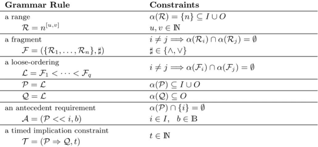
(P << i, false) F1< F2< F3 ({R1, R2}, ∧) n[1,1]1 n [1,1] 2 ({R1, R2}, ∨) n[2,8]3 n [1,1] 4 ({R1}, ∧) n[1,1]5

Attributes (for each node except the root):

- inherited: s, B, C, Ac, Af - synthesized:α Example for n[2,8]₃ : s= ∨ B = {n1, n2} C = {n4} Ac= {n5} Af= {i} α = {n3}

Figure 4: The property (({n1, n2}, ∧) < ({n [2,8] 3 , n4}, ∨) < n5<< i, false) s0 s2 s5 s1 s3 s4 start start.n.C/ [cpt=0] start.C/ [cpt=0] start.n/ [cpt=1] [s=∨] Ac/nok [cpt>=u] Ac/ok Ac/ok C/ n/ [cpt+=1] n/[cpt+=1] C/ [s=∧]Ac/err Af ∨ B/err Af∨B∨Ac/err [cpt<u]Ac∨ C/err Af∨ B/err [cpt=v]n/err [cpt>=u] C/ Af∨ B ∨ n/err C/ [cpt<v]n/ [cpt+=1] true/err

Figure 5: Elementary recognizer for a range R = n[u,v]_{: cpt is a counter;}

{start, n, B, Ac, Af, C} are inputs; {err, ok, nok} are outputs. Each transition

is of the form [condition]input/output[action] where input is a Boolean formula and output is a set.

Recognizers for Loose-Orderings Consider a loose-ordering L = F1 <

· · · < Fq. The recognizer of L is made by composing sequentially the recognizers

of the Fis: to start recognizing L, we have to send start to the recognizer of

F1; the output ok of the recognizer of Fi is connected to the input start of the

recognizer of Fi+1. The output ok of the last fragment signals the stop of the

recognizer of L.

SystemC Implementation Each node of the syntax tree of the formula is translated into a SystemC monitor. The monitor of a range encodes the state machine shown in Figure 5. Activation of the root monitor is propagated to monitors at lower levels. If any of the range monitors detects an error, the composite monitor of the property reports an error. The monitor of a timed implication constraint T = (P ⇒ Q, t) has two SystemC specific variables sc_core::sc_time start,stop. start is set to the current simulation time when P is recognized; stop is set to the current simulation time when the recognition of Q is finished; their difference should not be greater than T .

7

Experiments and Evaluation Results

Experimental Setting We consider two strategies to obtain monitors from loose-ordering properties: (i) Drct is the direct translation into SystemC (sec-tion 6); (ii) ViaPSL first translates the properties into PSL (sec(sec-tion 5); then the built PSL encodings are translated into SystemC monitors as described in [14, 5]. The time and memory complexities of the obtained monitors are compared: the former is measured in the number of operations executed by the monitors for each event observed, the later is defined by the number of bits needed to store the Boolean and bounded Integer variables.

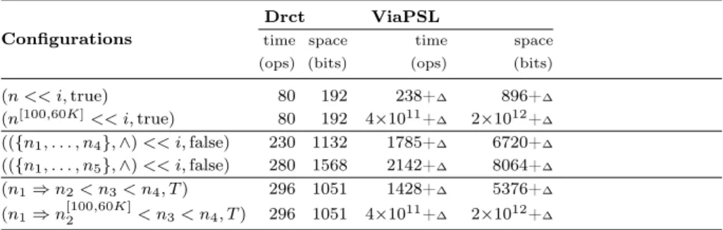
Configurations

Drct ViaPSL

time space time space (ops) (bits) (ops) (bits)

(n << i, true) 80 192 238+∆ 896+∆ (n[100,60K]_{<< i, true) 80 192 4×10}11_{+∆ 2×10}12_+∆ (({n1, . . . , n4}, ∧) << i, false) 230 1132 1785+∆ 6720+∆ (({n1, . . . , n5}, ∧) << i, false) 280 1568 2142+∆ 8064+∆ (n1⇒ n2< n3< n4, T ) 296 1051 1428+∆ 5376+∆ (n1⇒ n[100,60K]2 < n3< n4, T ) 296 1051 4×1011+∆ 2×1012+∆

Figure 6: Comparison of Drct and ViaPSL strategies

Comparison According to [14] the time and memory complexities of the monitors generated with the ViaPSL strategy are linear in the size of the formula; therefore they are equal to Θ(∆ +Pp

i=1(vi− ui+ 1)2+P q

α(Fj−1) |) with i (resp. j) ranging over all ranges Ri= n[ui,vi] (resp. fragments

Fj) of A or G, ∆ is a cost of translating ranges into new names.

The time complexity of the monitors generated with the Drct strategy is Θ(maxi∈[1..q]| α(Fi) |), i ranging over all the fragments of A (resp. G); “max”

is due to the fact that only monitors of the active fragment work while scanning a sequence. The space complexity of the monitor is Θ(Pq

i=1 | α(Fi) |) for both

Boolean and bounded unsigned Integer variables. The maximum value which can be assigned to any of these Integers is equal to max vi for all ranges Ri= n

[ui,vi]

i

of the pattern.

Figure 6 lists different configurations of the loose-ordering patterns used in the specification of our case-study (see section 3). The provided results show that our monitors have always smaller time/space complexities than the monitors obtained from PSL encodings. The presence of non-trivial ranges has no effect on the complexities of our Drct monitors, however their impact on the complexities of the ViaPSL monitors is huge.

8

Conclusion and Further Work

We defined the notion of loose-ordering for specifying the interactions between components. We proposed patterns to capture these properties and an encoding into SystemC monitors which is direct, and modular. The encoding is very effi-cient because it avoids size explosion, and fully exploits the fact that sub-formulas do not share names; when translating into PSL this structural information is lost. Future work will be devoted to a translation of the patterns into some code for generating random sequences. This will provide a full integration of loose-orderings in an ABV framework.

References

[1] Verisity Design e Reuse Methodology Developer Manual, 2002-2004. [2] Spot’s online ltl-to-tgba translator

spot.lrde.epita.fr/trans.html, 2015.

[3] I. S. 1850-2005. IEEE Standard for Property Specification Language (PSL), 2005.

[4] Universal verification methodology - www.accellera.org, 2012.

[5] Z. B. A. Amor. Validation de systèmes sur puce complexes du niveau trans-actionnel au niveau transfert de registers. Theses, University of Grenoble, 2014.

[6] P. Caspi, N. Halbwachs, D. Pilaud, and J. Plaice. Lustre, a Declarative Language for Programming Synchronous Systems. In 14th Symposium on Principles of Programming Languages, Munich, Jan. 1987.

[7] B. Cohen, S. Venkataramanan, and A. Kumari. Using PSL/Sugar for formal and dynamic verification: Guide to Property Specification Language for Assertion-based Verification. Cohen Publishing, 2004.

[8] M. Hansen and Z. Chaochen. Duration calculus: Logical foundations. Formal Aspects of Computing, 9(3):283–330, 1997.

[9] IEEE standard for SystemC language manual, 2011. Computer Society Std. [10] S. Iman and S. Joshi. The e hardware verification language. Dordrecht:

Kluwer Academic Publishers. xxii, 349 p., 2004.

[11] K. Morin-Allory and D. Borrione. On-line monitoring of properties built on regular expressions sequences. In S. A. Huss, editor, Advances in Design and Specification Languages for Embedded Systems (Selected Contributions from FDL’06), ISBN :978-1-4020-6147-9, pages 197–207. Springer, 2007. [12] M. F. Oliveira, C. Kuznik, H. M. Le, D. Große, F. Haedicke, W. Mueller,

R. Drechsler, W. Ecker, and V. Esen. The system verification methodology for advanced tlm verification. In Proceedings of the Eighth IEEE/ACM/IFIP CODES+ISSS, pages 313–322, New York, NY, USA, 2012. ACM.

[13] Open SystemC Initiative, SystemC Verification Library, 2014. v2.

[14] L. Pierre and L. Ferro. A tractable and fast method for monitoring SystemC TL specifications. IEEE Transactions on Computers, 57(10):1346–1356, 2008.