to the repository administrator: tech-oatao@listes-diff.inp-toulouse.fr

OATAO is an open access repository that collects the work of Toulouse researchers and makes it freely available over the web where possible

Any correspondence concerning this service should be sent

to the repository administrator: tech-oatao@listes-diff.inp-toulouse.fr

This is an author’s version published in: http://oatao.univ-toulouse.fr/23520

To cite this version:

Smith, Amy F. and Doyeux, Vincent and Berg, Maxime and Peyrounette, Myriam and Haft Javaheriam, Mohamad and Larue, Anne and Slater, John H. and Lauwers, Frédéric and Blinder, Pablo and Tsai, Philbert and Kleinfeld, David and Schaffer, Chris B. and Nishimura, Nozomi and Davit, Yohan and Lorthois, Sylvie Brain capillary networks across species : a few simple organizational requirements are sufficient to reproduce both structure and function. (2019) Frontiers in Physiology, 10 (233). 1-22. ISSN 1664-042X Official URL: https://doi.org/10.3389/fphys.2019.00233

O pen 1 \r<.;hivc 'l'uuluusc Archive Ouvcrlc (OA'l'AO)

Supplementary material for Brain capillary networks across species:

a few simple organizational re- quirements are sufficient to repro- duce both structure and function (2019) Frontiers in Physiology, doi:

10.3389/fphys.2019.00233.

by: Amy F. Smith, Vincent Doyeux, Maxime Berg, Myriam Peyrounette, Mohammad Haft-Javaherian, Anne-Edith Larue, John H. Slater, Frédéric Lauw- ers, Pablo Blinder, Philbert Tsai, David Kleinfeld, Chris B. Schaffer, Nozomi Nishimura, Yohan Davit and Sylvie Lorthois.

S1 Generation of 3D synthetic networks

S1.1 Generation of Voronoi diagram Each cell of length L

was divided into 16 × 16 × 16 pixels, and one seed was placed at a random pixel.

The 3D Voronoi diagram was extracted using the MATLAB function voronoin , which returns the co- ordinates of vertices and the list of vertices belonging to each polyhedron, from which the network connec- tivity matrix was constructed.

S1.2 Pruning the network

Very small or narrow polyhedral faces (with area

< 75 pixels or with any interior angle < 30 °) were merged with the neighboring face sharing the longest edge of the current face ie. this edge was deleted.

Similarly, neighbouring faces lying almost in a plane (solid angle < 15°) were merged. If any triangles with area < 75 pixels remained, the longest edge was removed. Final networks were not very sensitive to the choice of face area or angle criteria.

Vertices were then removed or merged in two stages:

1. Boundary vertices. If two boundary vertices v

and v

were located within some minimum dis- tance D

of each other, v

was arbitrarily

deleted, but only if it was connected to an inte- rior (i.e. non-boundary) vertex v

which had more than three connections. If both boundary vertices were connected to the same interior ver- tex v

, which itself only had three connections ( v

and v

plus one other interior vertex v

), then v

and v

were deleted, and v

was in- stead connected to v

. If neither of these cases applied, v

was moved a distance D

along the boundary away from v

in the direction of the vector between the two vertices.

2. Interior vertices. To minimize the computa- tionally heavy task of calculating the distance between all vertices, the domain was divided into sub-cubes of size L

× L

× L

(solid lines in 2D in Figure S1a). These cubes were shifted by 0.5L

in each direction yielding an off-set grid, to avoid missing vertex pairs span- ning neighboring cubes (dashed lines in Fig- ure S1a). Running through cubes in random- ized order, the distance between each pair of vertices within the same cube was calculated. If a pair of vertices ( v

and v

) lay < D

from each other, as in Figure S1b, v

was arbitrarily deleted and its connections were re-attached to v

(Figure S1c), but only if v

still had at least three connections. Otherwise, v

was moved a distance D

away from v

in the direction of the vector between the two vertices.

Final networks were not very sensitive to the choice of D

, and thus its value was fixed at 2.5 pixels (for L

= 75µm, D

= 11.7µm).

Next, excess edges between internal vertices were removed in random order according to the following criteria. An interior vertex could not have more than one connecting edge with a boundary vertex, except if it only had one internal connection, in which case it may be connected to two boundary vertices. If an internal vertex was not connected to any boundary vertices, it should have three connections to internal vertices.

S1.3 Splitting multiply-connected ver- tices

Vertices with more than 3 connections were treated

in random order. For each multiply-connected ver-

tex, the shortest connected edge was kept, as well

as the edge with smallest solid angle relative to that

(d) (e)

(f) (g)

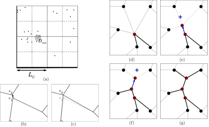
Figure S1: a) Schematic diagram illustrating the division of the domain into a grid of length L

(solid lines) and an off-set grid shifted by 0.5L

(dashed lines), for efficient detection of vertices (black dots) less than distance D

apart. b) Illustration of two vertices v

and v

separated by less than D

; c) vertex v

and its connections are merged into vertex v

; d) - g) Sequence of schematic diagrams illustrating the division of a multiply-connected vertex with five connections into three bifurcations. See text for further details.

edge (see e.g. the two edges in bold in Figure S1d).

The center of mass of the remaining vertices was calculated (the cross in blue in Figure S1e), and a new vertex was placed on the vector between the initial vertex and the center of mass, at a distance of half the shortest length of the remaining edges, or D

, whichever is smaller (see the blue arrow in Figure S1e). This process was repeated until all interior vertices had only three connections (Fig- ure S1f and g). This step introduced more short vessel lengths, but since there were typically only a small percentage of multiply-connected vertices, this did not have an important effect on overall network properties.

S1.4 Domain size

To avoid any boundary effects associated with the generation of these synthetic networks, for a desired

domain size of L

× L

× L

, a larger network was initially generated in a domain of 2(L

+ 2L

) × 2(L

+ 2L

) × 2(L

+ 2L

) (with L

rounded up to the nearest multiple of L

). At the end of the process, the desired sub-network in a domain of size L

× L

× L

was extracted from the center of the large domain.

S2 Results in lattice networks

Results for the two ordered, regular lattice net- works introduced in Section 2.2.2 and shown in Fig- ure 1Dare presented. These networks are referred to respectively as the CLN (with 6-connectivity) and the PLN (with 3-connectivity). After a study of the scaling properties of these networks, we present the results of metrics for chosen domain size and scaling.

'

_ _ _ _ _ _ _ .,L _ _ _ _ _ _ _

\.:" l

,D

.

---+--- '

--- - - -~ - -' ----

- - - -~ - - - -

'

(a)

(6) (c)

+

S2.1 Scaling of lattice networks

We first present an analytical investigation into the scaling of these networks with domain size or with mean length L . Recall that in both lattice networks, the length of the elementary cubes, L

, is linearly proportional to L (L

= L in the CLN and L

= 3L in the PLN).

The Voronoi-like synthetic networks, despite ex- hibiting greater randomness, also follow a similar semi-ordered structure controlled by the character- istic length L

. Thus we make the hypothesis that these metrics scale with L

in the same way, and use this to inform the scaling studies in Section 3.2.

S2.1.1 Morphometrical metrics

The mean vessel length was L for both lattice net- works. The length density was 3L/L

for the CLN and 30L/(3L)

for the PLN. Obviously, none of these metrics depended on domain size, in contrast to the loop metrics studied below.

S2.1.2 Topological metrics

The scaling of topological metrics with domain size was derived analytically. Loop metrics computed for lattice networks generated for the range of domain sizes shown in Figure S2 agreed perfectly with the analytical expressions derived in this section.

For both networks, we suppose that i , j and k are the number of unit cells in the x, y, and z di- rections respectively. Both lattice networks had two modes of loops, α = 1, 2 , with m

edges per loop.

We then define the mean number of edges per loop, N

(i, j, k) , as the total number of loop edges, divided by the total number of loops, i.e.:

N

= P

α=1

m

N

(i, j, k) P

α=1

N

(i, j, k) , (S1) where N

(i, j, k) are the number of loops corre- sponding to mode α.

Similarly the mean loop length, L

, was given by:

L

= L × N

,

and thus converged with domain size in the same way as N

(i, j, k) , but also scaled with L .

The mean number of loops per edge, N

(i, j, k), is the total number of loop

edges divided by the number of interior (i.e.

non-boundary) edges, N

(i, j, k):

N

= P

α=1

m

N

(i, j, k)

N

(i, j, k) . (S2) These metrics were derived for the specific geome- tries of the CLNs and PLNs as follows.

Cubic lattice network The CLN had two modes of loops with 4 and 6 edges respectively ( m = { 4, 6 }). The number of loops with 4 edges, N

(i, j, k) , followed:

N

(i, j, k) = i(j − 1)(k − 1) + (i − 1)j(k − 1) + (i − 1)(j − 1)k,

for i, j, k > 0 . Similarly, the number of loops with 6 edges, N

(i, j, k), obeyed:

N

(i, j, k) = R (i(j − 1)(k − 2)) + R (i(k − 1)(j − 2)) + R (j(i − 1)(k − 2)) + R (j(k − 1)(i − 2)) + R (k(i − 1)(j − 2)) + R (k(j − 1)(i − 2)) . where R(x) is the ramp function, defined as:

R(x) =

( x, x ≥ 0;

0, x < 0.

Using Equation S1, the mean number of edges per loop for a cube of side length n = i = j = k and n ≥ 2 was given by:

N

= 4 × 3n(n − 1)

+ 6 × 6n(n − 1)(n − 2) 3n(n − 1)

+ 6n(n − 1)(n − 2)

→ 5

/

as n → ∞ .

The mean number of edges per loop converged to within 5% of the converged value for networks of 4

unit cubes (Figure S2a).

In this network, the number of interior (i.e. non- boundary) edges, N

(i, j, k), was given by:

C := R ((i − 1)jk) + R (i(j − 1)k) + R (ij(k − 1)) .

(S3)

(a) (b)

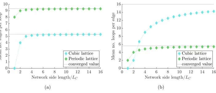
Figure S2: Scaling of lattice networks with domain size. a) Mean number of edges per loop, N

, and b) mean number of loops per edge, N

, in the CLNs and PLNs as a function of the number of unit cells. Analytical and numerical results agreed exactly. The converged values for each metric and network, computed analytically, are plotted in gray lines.

This quantity C will also be used later. Then, substituting this expression into Equation S2 with n = i = j = k and n ≥ 2 , N

becomes:

N

= 4 × 3n(n − 1)

+ 6 × 6n(n − 1)(n − 2) 3n

(n − 1)

→ 16 as n → ∞ .

Convergence was slow: this metric was only con- verged to within 5% of this value for networks of 36

unit cubes or greater (Figure S2b).

Periodic lattice network Next, analytical ex- pressions for the same loop metrics were derived for the PLN, which had two modes of loops with 8 and 10 edges respectively (m = { 8, 10 }). The number of loops with 8 edges, N

(i, j, k) , followed:

N

(i, j, k) = 6ijk,

while the number of loops with 10 edges, N

(i, j, k) , obeyed:

N

(i, j, k) = 4C,

where C is defined in Eqn. S3. Using Equation S1, when n = i = j = k and n ≥ 2 , N

becomes:

N

= 8 × 6n

+ 10 × 12n

(n − 1) 6n

+ 12n

(n − 1)

→ 9

/

as n → ∞ .

N

quickly converged to within 5% of this value for networks of 2

unit cubes (Figure S2a).

In this network, N

(i, j, k) here was given by:

N

(i, j, k) = 24ijk + 2C.

Then, using Equation S2, and with n = i = j = k and n ≥ 2, N

becomes:

N

= 8 × 6n

+ 10 × 12n

(n − 1) 24n

+ 6n

(n − 1)

→ 5.6 as n → ∞ .

N

converged more quickly for the PLN than the CLN, and was within 5% of its converged value for networks of 11

unit cubes or more (Figure S2b).

Thus, in both lattice networks the number of loops per edge was especially sensitive to finite-size effects.

Nonetheless, none of the loop metrics except the mean loop length depended on the choice of L (or equivalently L

), and thus are purely topological metrics.

S2.1.3 Permeability

Cubic lattice network In the CLN, imposing a pressure gradient in the x -direction yields zero flow in vessels orientated parallel to the y - or z -axis: the network is reduced to an array of tubes of length L

10

16

9 . / •

14 ••••••

0.. 0

8

• - • •

,Q

a:5 12

·-··

I-<

7

•

Q) Q) • • ✓·•

0..

6

00 00

•-

Q) 0..

bO

5 •

⁸ I

"Cl Q) ,Q

g ⁴ ✓ ^{0 6 •}

3

I

^{!+ • - •}

i::: i:::

ro I ^• Cubic lattice ^ro 4 .,v

• Cubic lattice

Q)

2

^{/ I}

::E

• Periodic lattice ::E 2 • -

•

^• Periodic lattice

1 I _{- converged value}

_- converged value

0 0

0 2 4 6 8

12 14 16 0 2 4 6 8

12 14 16

Network side length/ Le Network side length/ Le

where L

is the ROI size in the x -direction. The global flowrate Q

is:

Q

= N πd

128µ × ∆P

L

(S4)

where µ is the effective viscosity, d is the diame- ter (which here is uniform), and ∆P is the pressure drop. N is the number of boundary vessels on the face x = 0, expressed in terms of L, the edge length:

N = L

L × L

L . (S5)

From Equation (1), this yields:

K

= µ

∆P/L

× L

L

A

L

× πd

128µ

∆P L

. (S6) Rearranging and using the definition for the domain area perpendicular to the x -axis, A

= L

L

, gives:

K

= πd

128L

. (S7)

Figure S3: Flow distribution in an elementary motif of the PLN with a pressure gradient from left to right. The magnitude of the flow in the green vessels was half of that in the red vessels, and zero in the dark blue vessels.

Periodic lattice network In the PLN, imposing a pressure gradient in the x -direction with uniform diameters also yields a simple flow distribution (Fig- ure S3 and legend). The global flowrate obeys the same law in Equation S4, but N follows:

N = 2L

3L × L

3L . (S8)

In the minimal example shown in Figure S3, L

= 3L and L

= 3L giving N = 2 . Substituting this expression into Equation (1) yields:

K

= 2

9 × πd

128L

. (S9)

Thus, to obtain the same permeability in both lat- tice networks, L in the PLN would have to be

√

2

/

= 0.47 times that of the CLN.

Finally, for both lattice networks, the permeabil- ity scaled with d

and

/

(or equivalently

/

)and did not depend on domain size (assuming uniform diameters).

S2.2 Lattice networks scaled to match mouse ROIs

In the CLN, L = 67µ m was chosen to match the length density in mice. A network of 4 × 4 × 4 unit cubes was generated with dimensions 268 × 268 × 268µ m

, to be as close as possible to the size of the mouse ROIs will containing whole unit cubes. In the PLN L = 41µm; with the unit cube side length being L

= 3L , a network of 2 × 2 × 2 unit cubes was generated with dimension 246 × 246 × 246µ m

. Results in these networks are given in Table 1.

Space-filling metrics In the box-counting anal- ysis, the cut-off lengths for both lattice networks were of a similar order of magnitude to the other networks, but in contrast, both had linear regimes at small scales. The mean EVD was very close to the mouse data for both lattice networks, while the maximum EVD was lowest in the CLN, and high- est in the PLN. The mean local maxima of EVDs were 22% and 61% higher in the PLNs and CLNs respectively.

Morphometrical metrics The PLN had a sim- ilar mean length to that in mice, while that in the CLN was almost 50% higher. By construction, the length distributions in these networks were drasti- cally different to the mouse and synthetic networks, with only one mode for each network, and hence zero SD. Due to the choice of L as described above, the mean length density in both networks was very close to that in mice. As a result, in the PLN both the edge density and vertex density were close to those in mice, whereas the CLN had a much lower edge and vertex density. Both lattice networks had a much lower density of boundary vertices (36% and 62% respectively).

Topological metrics By construction the PLN had no multiply connected vertices, while all junc- tions in the CLN had 6 connections. The distri-

r

7

I I

I

bution of loops was very different for the lattice networks, with fewer edges per loop (9 and 5.14 respectively) on average, with values restricted to two modes per network, as described above in Sec- tion S2.1.2. The mean loop length was also lower in both lattice networks than in mice.

Flow metrics The mean velocity was 45% higher in both the lattice networks. Similarly, the mean permeability in the PLNs and especially the CLNs was much higher than in mice (almost 30% and 120% higher respectively), and completely isotropic due to their regular construction.

Mass transfer metrics Unsurprisingly, the dis- tribution of capillary transit times for lattice net- works were very different to those in the synthetic and mouse ROIs (Figure 8E). The exchange coeffi- cient h was 26.5% and 32.9% higher in the PLNs and CLNs respectively compared mice.

Robustness metrics For the PLN, the histogram of pre- to post-occlusion flow ratios was very differ- ent to the distributions for the mice and synthetic networks, due to its highly organized architecture (Figure 8F), and was restricted to 3 modes. The mean flow ratio was approximately 10% lower than in mice. The CLN was not included because none of its vertices were converging bifurcations.

In conclusion, while some simple morphometri- cal metrics in the lattice networks aligned well with those in mice, their highly organised structure meant that the distribution of metrics was completely dif- ferent, and topological and functional metrics also differed greatly from the more randomized networks.

Thus, such simple networks cannot be used to make

accurate predictions of functional properties in the

cerebral capillaries.

Supplementary Figures and Tables

(a) (b)

Figure S4: Convergence of metrics with domain size in the synthetic networks: a) mean loop length, b) length density. Metrics were normalized by the appropriate power of L

. Insets: the convergence of each metric as defined in Equation 2. The converged size x

is the size from which the convergence was less than 0.05.

(a) (b)

(c) (d)

Figure S5: Scaling of metrics with the characteristic length L

in the synthetic networks: a) mean loop length, b) edge density, c) mean number of edges per loop, d) mean number of loops per edge. Errorbars show mean ± S.D. for the synthetic networks. Shaded bands in blue and red show mean ± S.D. of mouse and human values respectively.

0 60

.J-1-+-t+-J·-f--•--H-

/ -•--•-·•-·•

65 70 75 80 85 Le, µm

8 9

95 100

---t---:+.-::r::_, __ :_-r ···-···

----+--+----1

0

60 65 70 75 80 85:--_...,=::;::.~

Le, µm 95 100

100-390-0 3

6

0

60 65 70 75

__ --½

__

..,--- .. ^---

80 -;:85;:---'-'~~~

Le, µm 95 100

(a) (b)

Figure S6: Space-filling results for human and synthetic with L

= 90µ m networks. a) Box counting results for local maxima of EVDs. For a regular grid of cubic elements of side r , N is the number of square elements containing at least one local maxima. Dotted vertical lines show the value of x

for each species, above which the slope is -3. b) Histogram of EVDs, collected over all ROIs, on a log-log scale.

Metric Human S90

N 4 10

Mean EVD (µm) 21.4 ± 0.6 24.1 ± 1.0

Mean local max EVD (µm) 33.3 ± 1.0 40.2 ± 3.1

Max EVD (µm) 52.9 ± 0.7 63.2 ± 2.7

Convexity index 0.8 ± 0.1 0.7 ± 0.2

Mean length (µm) 60.2 ± 3.1 41.9 ± 1.8

SD length (µm) 41.7 ± 0.8 21.4 ± 2.0

Edge density (10

mm

) 8.4 ± 0.4 11.9 ± 0.9

Length density (mm

) 461 ± 19 442 ± 28

Vertex density (10

mm

) 3.9 ± 0.2 6.3 ± 0.5 Boundary vertex density (mm

) 207 ± 8 186 ± 16

% multiply-connected vertices 2.9 ± 1.7 2.6 ± 1.6

Mean no. edge/loop 11.2 ± 0.6 10.2 ± 0.6

Mean loop length ( µ m) 635 ± 73 429 ± 34

Mean no. loop/edge 3.1 ± 0.6 4.4 ± 0.5

Mean velocity (µm/s) 148 ± 34 202 ± 26

SD velocity (µm/s) 223 ± 34 228 ± 18

Permeability (10

µm

) 0.62 ± 0.21 0.86 ± 0.13 Median transit time (s) 0.19 ± 0.06 0.14 ± 0.02 Exchange coefficient h 27.7 ± 3.71 15.7 ± 1.12 Post-occlusion flow ratio (converging) 0.77 ± 0.03 0.76 ± 0.01 Post-occlusion flow ratio (diverging; branch A) 0.28 ± 0.05 0.28 ± 0.04

Table S1: The geometrical, topological and functional metrics calculated here, for human and synthetic with L

= 90µ m (‘S90’) networks. Results are presented as mean ± S.D. over the N ROIs studied for each network type. Permeabilities, velocities and transit times were calculated with uniform diameters of 5µm.

10•

.,, 103

~

al

j

.s

'cl tl 101

1

Z -!-S90 10"

10" 10¹

Box size, µm

101

10-• 1- Humanl -•-S90

10-⁵ ~ - - - ~ - - - -~ ~

10¹

Extravasculax distance, µm

(a) (b)

(c) (d)

(e)

Converging

{

Diverging

{

Diverging

Converging

(f)

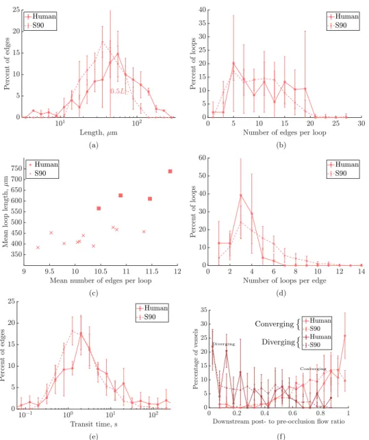
Figure S7: Results for human ROIs and synthetic networks (‘S90’) with L

= 90µ m and domain size 264 × 264 × 207µ m

. a) Histogram of lengths on a log-scale. Frequencies collected over all ROIs for each network type. b) Histogram of number of edges per loop. c) Mean loop length, µm, vs. mean number of edges per loop, for each ROI. d) Histogram of number of loops per edge. e) Histogram of capillary transit times, on a log-scale. f) Histograms of post- to pre-occlusion absolute flow ratios in vessels one branch downstream from the occlusion, where the vertex downstream of the occlusion has 3-connectivity, and divided into converging and diverging bifurcations. In the diverging case, flow ratios are plotted for the outflow branch without change in flow direction post-occlusion.

25, ~ - - ~ + Human 20 -!-S90

750 ^{1 ·} Humanl

· S90 Ei 700

~

£650 g>600 -;_ 550 ] 500

§ 450

:;E

9 9.5

Length, µm

• •

•

X

10 10.5 11 11.5 Mean number of edges per loop 25

20

"'

al

"""' ⁰ ] 10

~

<1)

P,

5

0 10-1 10'

Transit time, s

+ Human -!-S90

•

12 40 35

00 30

0.

] 25

"o 20

"'=

~ 15

<1)

P, 10 5 0 0

60 50

00

§'40 .Q

"o 30

"'= ^<1)

~ 20

P,

10 0 0

35 30

5

2

0.2

10 15 20

+ Human -!-S90

25 30

Number of edges per loop

-+,,,!--- -- --

4 6 8 10

+ Human -!-S90

12 14 Number of loops per edge

0.4 0.6

+Human -!-S90 +Human -!-S90

0.8 Downstream post- to pre-occlusion flow ratio

Metric Unit n α β R

Length density mm

-2 3.70× 10

0.61 0.996

Mean EVD µm 1 0.26 0.33 0.991

Permeability µ m

-2 9.43 -2.05× 10

0.995 Mean loop length µm 1 4.45 23.23 0.971

Mean length µm 1 0.41 4.27 0.991

Edge density mm

-3 8.20×10

1.21×10

0.998

Table S2: In the synthetic networks, results of a standard linear regression on a range of metrics as a

function of L

to the appropriate power, i.e. following the expression: αL

+ β , where n is the power

appropriate for each metric. The coefficient of determination, R

, was very good for all fits.