to the repository administrator: tech-oatao@listes-diff.inp-toulouse.fr

OATAO is an open access repository that collects the work of Toulouse researchers and makes it freely available over the web where possible

Any correspondence concerning this service should be sent

to the repository administrator: tech-oatao@listes-diff.inp-toulouse.fr

This is an author’s version published in: http://oatao.univ-toulouse.fr/23520

To cite this version:

Smith, Amy F. and Doyeux, Vincent and Berg, Maxime and Peyrounette, Myriam and Haft Javaheriam, Mohamad and Larue, Anne and Slater, John H. and Lauwers, Frédéric and Blinder, Pablo and Tsai, Philbert and Kleinfeld, David and Schaffer, Chris B. and Nishimura, Nozomi and Davit, Yohan and Lorthois, Sylvie Brain capillary networks across species : a few simple organizational requirements are sufficient to reproduce both structure and function. (2019) Frontiers in Physiology, 10 (233). 1-22. ISSN 1664-042X Official URL: https://doi.org/10.3389/fphys.2019.00233

O pen 1 \r<.;hivc 'l'uuluusc Archive Ouvcrlc (OA'l'AO)

Edited by:

Antonio Colantuoni, University of Naples Federico II, Italy

Reviewed by:

Dominga Lapi, University of Pisa, Italy Alla B. Salmina, Krasnoyarsk State Medical University named after Prof.

V.F.Voino-Yasenetski, Russia

*Correspondence:

Sylvie Lorthois lorthois@imft.fr

Specialty section:

This article was submitted to Vascular Physiology, a section of the journal Frontiers in Physiology

Received:27 September 2018 Accepted:22 February 2019 Published:26 March 2019

Citation:

Smith AF, Doyeux V, Berg M, Peyrounette M, Haft-Javaherian M, Larue A-E, Slater JH, Lauwers F, Blinder P, Tsai P, Kleinfeld D, Schaffer CB, Nishimura N, Davit Y and Lorthois S (2019) Brain Capillary Networks Across Species: A few Simple Organizational Requirements Are Sufficient to Reproduce Both Structure and Function.

Front. Physiol. 10:233.

doi: 10.3389/fphys.2019.00233

Brain Capillary Networks Across

Species: A few Simple Organizational Requirements Are Sufficient to

Reproduce Both Structure and Function

Amy F. Smith¹, Vincent Doyeux¹, Maxime Berg¹, Myriam Peyrounette¹,

Mohammad Haft-Javaherian², Anne-Edith Larue¹, John H. Slater³, Frédéric Lauwers^4,5, Pablo Blinder⁶, Philbert Tsai⁷, David Kleinfeld⁷, Chris B. Schaffer², Nozomi Nishimura², Yohan Davit¹and Sylvie Lorthois^1,2*

1Institut de Mécanique des Fluides de Toulouse (IMFT), Université de Toulouse, CNRS, Toulouse, France,²Nancy E. and Peter C. Meinig School of Biomedical Engineering, Cornell University, Ithaca, NY, United States,³Department of Biomedical Engineering, University of Delaware, Newark, DE, United States,⁴Toulouse NeuroImaging Center (TONIC), Université de Toulouse, INSERM, Toulouse, France,⁵Department of Anatomy, LSR44, Faculty of Medicine Toulouse-Purpan, Toulouse, France,⁶Department of Neurobiology, George S. Wise Faculty of Life Sciences, Tel-Aviv University, Tel Aviv, Israel,

7Department of Physics, University of California, San Diego, La Jolla, CA, United States

Despite the key role of the capillaries in neurovascular function, a thorough characterization of cerebral capillary network properties is currently lacking. Here, we define a range of metrics (geometrical, topological, flow, mass transfer, and robustness) for quantification of structural differences between brain areas, organs, species, or patient populations and, in parallel, digitally generate synthetic networks that replicate the key organizational features of anatomical networks (isotropy, connectedness, space-filling nature, convexity of tissue domains, characteristic size). To reach these objectives, we first construct a database of the defined metrics for healthy capillary networks obtained from imaging of mouse and human brains. Results show that anatomical networks are topologically equivalent between the two species and that geometrical metrics only differ in scaling. Based on these results, we then devise a method which employs constrained Voronoi diagrams to generate 3D model synthetic cerebral capillary networks that are locally randomized but homogeneous at the network-scale.

With appropriate choice of scaling, these networks have equivalent properties to the anatomical data, demonstrated by comparison of the defined metrics. The ability to synthetically replicate cerebral capillary networks opens a broad range of applications, ranging from systematic computational studies of structure-function relationships in healthy capillary networks to detailed analysis of pathological structural degeneration, or even to the development of templates for fabrication of 3D biomimetic vascular networks embedded in tissue-engineered constructs.

Keywords: cerebral cortex, capillary network, capillary loop, capillary network model, biomimetic network

OPEN ACCESS

1. INTRODUCTION

Archaeologists can understand past human economic and socio- political behavior, or resilience of ancient societies to strong perturbations such as repeated drought, from the organization of their infrastructures such as roadways, water supply or sewage networks (Dillehay and Kolata, 2004). In the same way, the mechanisms of cognition in health and disease might ultimately be informed by studying the brain micro-vascular system.

This system provides a highly integrated and dynamic infrastructure for the distribution of blood: it supplies oxygen, nutrients and, in some cases, drugs to every cell in the brain, and ensures the removal of metabolic waste. Since the brain lacks any substantial energy reserve, the cerebral microcirculation also acts as a short-term regulation system, which responds quickly and locally to the metabolic needs of neurons (Hillman, 2014;

Rungta et al., 2018). In imaging neuroscience, changes in blood supply are thus considered as a surrogate for changes in neuronal activity, providing a unique way to observe the functioning brain.

The brain microvascular system is also involved in disease, including stroke and neurodegenerative disease, through vascular damage, such as capillary occlusions and progressive rarefaction (Østergaard et al., 2016; Cruz Hernández et al., 2019), and decrease in regulation efficiency (Farkas and Luiten, 2001; Iadecola, 2004). Together, these act to reduce blood flow and the availability of vital nutrients, which, on one hand, plays a key role in disease progression (Zlokovic, 2011;

Cruz Hernández et al., 2019) and, on the other hand, makes it difficult to interpret functional imaging data in patient populations (D’Esposito et al., 2003).

Consistent with its functions of distribution and exchange, the microvascular system includes several architectural components.

The arterioles form a quasi-fractal hierarchy of vessels (Nishimura et al., 2007; Blinder et al., 2010; Lorthois and Cassot, 2010; Shih et al., 2015) whose diameter decreases at each successive bifurcation, thus minimizing the time for supplying resources (Lorthois and Cassot, 2010). These vessels feed into the capillary network, a dense, mesh-like, three-dimensional (3D) interconnected structure, which is space-filling above a characteristic length scale of order 25− 75µm (Lorthois and Cassot, 2010). This ensures that no point in the tissue is further than half this characteristic length from the nearest vessel, due to the diffusion-limited distance of oxygen transport in oxygen consuming tissue. Their mesh-like structure gives the capillaries, the smallest vessels in the vasculature with a diameter∼5µm, an extremely large surface area facilitating their vital role in nutrient exchange (Popel and Johnson, 2005). De-oxygenated blood then drains into the venules, which broadly mirror the architecture of the arterioles.

These basic principles apply to a large variety of mammals, from rodents to humans, where the main difference in vascular organization described so far is the ratio between arterioles and venules which feed/drain a given region (Hartmann et al., 2017). Beyond these principles, thorough characterization of microvascular structure in the cortex is still incomplete. Thanks to the increasing number of vascular anatomical datasets in the literature (e.g., Cassot et al., 2006; Mayerich et al., 2008; Tsai

et al., 2009; Blinder et al., 2013; Xiong et al., 2017; Di Giovanna et al., 2018), the arterioles and venules both within the cortex (Cassot et al., 2010; Hirsch et al., 2012; Lorthois et al., 2014b) and at the level of the pial surface (Blinder et al., 2010) have been rigorously analyzed. However, despite their key role in supplying neurons with the required nutrients, there has been much less focus on the dense, complex mesh of capillaries. Previous studies of 3D cortical capillaries have principally been qualitative (e.g., Duvernoy et al., 1981), or limited to the characterization of global spatial properties, such as their space-filling nature, density, or diameter and length distributions (Lauwers et al., 2008; Lorthois and Cassot, 2010), with few insight on topology. One notable exception (Blinder et al., 2013) studied minimal loops and vessel resistance distributions to conclude that the capillaries form a highly interconnected mesh with no structural correlation to the location of cortical columns.

As a result, current understanding of the architectural organization of healthy brain capillary networks within the cortex is limited to a few striking features:

1. Brain capillary networks are approximately isotropic anastomosing networks whose vertices mainly have three connections (e.g.,Duvernoy et al., 1981; Blinder et al., 2013);

2. They are space-filling above a cut-off length of order 25− 75µm (e.g.,Lorthois and Cassot, 2010);

3. They approximately demarcate convex tissue domains with a characteristic length of similar order (in contrast to tumor networks whose tissue domains are multi-scale in nature, e.g., Baish et al., 2011).

This makes it difficult to build a precise mental representation of these networks that can materialize into a relevant generic capillary network model (orgeometric archetype in the words of Baish et al., 2011). Besides a better understanding of the fundamental organization of the cortical capillaries, such a generic network model is also needed for fundamental studies focused on understanding how structural differences between brain areas, organs, species or patient populations translate into functional differences with regard to blood flow, blood/tissue exchange, and associated imaging signals, e.g., in BOLD fMRI.

Similarly, implementation of image-guided, biofabrication techniques (Brandenberg and Lutolf, 2016; Heintz et al., 2016, 2017; Pradhan et al., 2017; Hoon et al., 2018) provides the ability to generate 3D, biomimetic vascular networks embedded in tissue-engineered constructs. These microphysiological systems could be useful for investigating the impact of capillary architecture and hemodynamics on complex biological processes in the brain, e.g., transport across the blood brain barrier.

Hence, the goals of this paper are:

1. To thoroughly characterize the structure and function of healthy cerebral capillary networks in both mice and humans, thereby identifying the similarities;

2. To generate synthetic capillary networks with equivalent properties via a generic method which is not tuned to a specific dataset, thereby evidencing key common organizational features among mice and humans.

These goals are inherently inter-linked and must be developed in parallel, to overcome the following challenge. A geometric archetype is necessary to guide definition and scaling of an appropriate set of metrics for characterizing both the structural and functional properties of brain capillary networks. On the other hand, thorough characterization of these properties from real experimental data is needed to ensure the relevance of this geometric archetype.

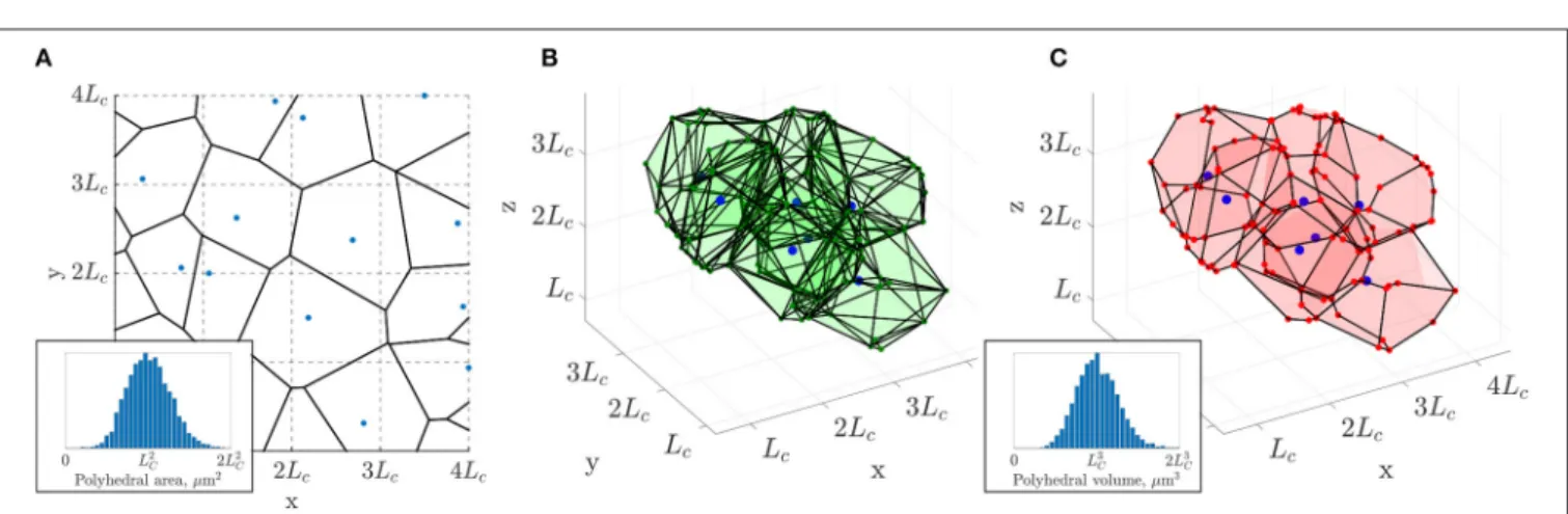
Therefore, the present paper is organized as follows. First, we describe the anatomical capillary datasets from mice and human cerebral cortex (section 2.1; mouse data shown inFigures 1 A-C).

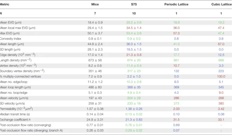
Then, we postulate that the current understanding of their architectural organization, as described by the three general features above, is sufficient to generate model networks replicating not only the morphological and topological properties of cerebral capillary networks, but also their flow and transport properties. Based on this postulate, we introduce in section 2.2, a constrained Voronoi-based method for generating 3D synthetic capillary networks with these three features, as summarized in Figure 2. Simpler, periodic grid-like lattice networks are also introduced (Figure 1D) to enable analytical derivation of metrics and associated scaling properties.

In section 2.3, we present a comprehensive set of quantitative metrics enabling characterization of network structure and function, that is: morphometrical metrics for the tissue (e.g., mean extravascular distances) and the capillary network (e.g., mean vessel length, length density); topological metrics (e.g., number of edges per capillary loop); flow metrics (e.g., velocity, permeability); mass transfer metrics (e.g., intravascular transit times, mass exchange coefficient) and robustness to occlusions (post vs. pre-occlusion flow ratio).

In the Results, these metrics are used in combination to demonstrate that, with appropriate scaling, mice and human capillary networks have similar properties. Moreover, we show that these properties can be matched by synthetic networks, and even to some extent simple lattice networks, demonstrating that only a few organizational requirements are sufficient to fully reproduce the fundamental properties of cerebral capillary networks.

2. MATERIALS AND METHODS

As described above, we first introduce the anatomical datasets used (section 2.1), then present the methods for generation of synthetic and lattice networks (section 2.2), before defining the metrics used to quantify and compare network properties (section 2.3). For clarity, in the latter sections, we focus on the general strategy and highlight the main ingredients. Further details not essential for understanding the present approach are given in section S1 of the Supplementary Material and in Appendix A, respectively. Unless otherwise indicated, the procedures described were implemented in a custom-built C++

code (Peyrounette et al., 2018).

2.1. Anatomical Datasets

Firstly, capillary ROIs were manually extracted from mouse and human anatomical datasets as follows.

2.1.1. Mouse Data

Vascular networks from the mouse somatorsensory cortex were previously obtained using a morphological-preserving vascular cast protocol (Tsai et al., 2009; Blinder et al., 2013). Briefly, the animals were euthanized with an overdose of pentobarbital. They were transcardially perfused at a rate of 0.5 ml/s to match the mouse heart output, with warm (37^◦C) saline until all blood was cleared (∼40–50 ml) and then with an excess of 20 ml of vascular casting perfusate, previously prepared by conjugating fluorescein-labeled-albumin (no. A9771; Sigma) with a 2% (w/v) solution of porcine gelatin (no. G1890; Sigma). The gel was allowed to solidify for 15 min while the animal was tilted down and immersed in an ice-cold water bath. Next, the head was severed at the level of the neck and moved overnight for fixation in 4% paraformaldehyde (PFA). The following day, the brain was removed from the skull under a fluorescent binocular (Zeiss Discovery 8). In order to preserve the dura and pial vasculature intact, the dissection was conducted guided by the fluoresce signal from the vascular cast which allowed the careful identification of dura to skull attachment places that were crucial to disconnect prior to removal of the corresponding skull bone.

Importantly, the bone was removed in small fractions, starting from the dorsal aspect and working in a circular fashion while progressing rostral until the whole brain was exposed. The brain was then moved back to PFA for 24 h. Images of the pial vasculature were obtained to serve as reference for subsequent optical sectioning of thick slabs, using two-photon laser scanning microscopy (TPLSM), at a resolution of 1 µm³. After data segmentation and vectorization of the vascular networks as described byTsai et al. (2009), vessel diameters were corrected to match values observedin vivousing an histogram matching approach (Cruz Hernández et al., 2019).

Arterioles and venules within the cortex were differentiated from the capillary mesh by manually classifying surface arteries/veins and then following connecting vessels downstream/upstream while vessel diameter was above a specified minimum threshold (7.2 µm), chosen for this dataset so that the resulting trees did not contain any loops (Cruz Hernández et al., 2019). Seven ROIs were selected from two cortical zones at cortical depths of over 650µm, to avoid vessels classified as arterioles and venules and extract the largest possible sections which only contained capillaries. Nonetheless, ROIs were limited to a size of 240×240×240µm³. The location of three such ROIs are shown inFigure 1A.

2.1.2. Human Data

Human data was obtained from the lateral part of the collateral sulcus (fusiform gyrus) of the temporal lobe as described in Cassot et al. (2006). Briefly, 300µm-thick sections of a human brain injected with Indian ink, from the collection of Henry Duvernoy (Duvernoy et al., 1981), were imaged by confocal laser microscopy, with a spatial resolution of 1.22× 1.22× 3 µm. The brain came from a 60 year old female who died from an abdominal lymphoma with no known vascular or cerebral disease. The procedures used to obtain a complete automatic reconstruction of the vascular network in large volumes (1.6 mm³) of cerebral cortex, i.e., mosaic M1 inCassot et al. (2006)

FIGURE 1 | (A)Section of mouse cerebral cortex fromTsai et al. (2009), viewed from above the pial surface (upper section of cortex and surface vessels removed for visualization purposes) and with vessels color-coded according to diameter. Three regions of interest (ROIs) of size 240×240×240µm³are outlined in fuschia.

(B)One ROI in further detail, with the same color scheme.(C)The same ROI with vessels straightened. Tortuosity was ignored in our analysis of network properties.

(D)Simple, periodic grid-like lattice networks enable analytical derivation of scaling properties (see section 2.2.2): CLN with 2×2×2 elementary cells (left), and 1 elementary cell of the PLN (right).

FIGURE 2 |3D extension of the 2D constrained Voronoi method ofLorthois and Cassot (2010).(A)Example of a 2D Voronoi diagram (thick black lines) generated from an array of seed points (in blue), one randomly placed in each cell with side lengthL_Cof a square grid (dashed lines). Inset: the distribution of polygonal areas, collected over 80 networks of size (3.2L_c)², followed a Gaussian distribution with mean of approximatelyL²_C(4473 polygons in total).(B)In 3D, a subset of polyhedra of the Voronoi diagram generated from the seed points in blue, one randomly placed in each cell with side lengthL_Cof a cubic grid (not showing all polyhedra for visualization purposes).(C)The same polyhedra with faces merged according to minimum angle and face area criteria as detailed in section 2.2 and section S1 of the Supplementary Material. Inset: the distribution of polyhedral volumes, collected over 10 networks of size (3.2L_C)³, followed a Gaussian distribution with mean approximatelyL³_C(4, 408 polygons in total).

A B

A B C

3Lc 3Lc

N 2Lc "' 2Le

Le Le

~L

Polyhedral area, µm² 2Lc 4Lc

3Le y ^{2Le Le Le 2Le} _X ^{3Le 0}

~

.. ^~

Polyhedral volume, µm³ X

X

have been described in detail elsewhere (Cassot et al., 2006;

Fouard et al., 2006). The mean radius and length of each segment were rescaled by a factor of 1.1 to account for the shrinkage of the anatomical preparation (Lorthois et al., 2011a). The main vascular trunks were identified manually and divided into arterioles and venules according to their morphological features, following Duvernoy’s classification (Duvernoy et al., 1981; Reina De La Torre et al., 1998). Arteriolar (resp. venular) trees within the cortex were then differentiated from the capillary mesh as above, with a threshold value of 9.9µm (Lorthois et al., 2011a).

From this classification, the largest possible capillary-only zones were identified, being limited in thexandydirections by the need to avoid arterioles and venules, and in thez-direction by the imaging depth. Since the slice of cortex studied was originally selected for its many large arborescences, this made difficult the extraction of capillary-only zones. Only four ROIs, of size 264× 264×207µm, were identified, one at a cortical depth of 300µm and three at a depth of over 1 mm. These regions were segmented from the raw images using DeepVess (Haft-Javaherian et al., 2019), a 3D deep convolutional neural network architecture for vasculature segmentation. The segmentation was then manually corrected by direct comparison with the raw images in Avizo to ensure that the network connectivity was well-reproduced.

Despite this, the final segmentation was inevitably less reliable for vessels near the limit of the confocal imaging depth due to the associated attenuation.

2.2. Synthetic Capillary Networks

As summarized in the Introduction, we hypothesize that the minimal organizational requirements of healthy cerebral capillary networks are that they are isotropic, three- connected and space-filling with approximately convex extravascular domains. The physiological hypothesis is that this ensures that no point in the oxygen consuming tissue is further than the diffusion-limited distance of oxygen transport from the nearest vessel.

To generate such networks, a method was sought to derive a tessellation of space into semi-regular “supply regions,” where capillaries lie along the boundaries separating these regions.

Voronoi diagrams provide a simple way to achieve this, as illustrated in Vrettos et al., 1989; Kou and Tan, 2010; Wu et al., 2012, and have been previously employed to generate 2D capillary networks (Lorthois and Cassot, 2010). We first present this method and its generalization to 3D, before defining grid- like lattice networks whose properties can be studied analytically.

All these networks are defined up to a constant factor, the characteristic lengthLC, which only controls the network scaling, and has no impact on topology. The exact choice of LC is non-trivial and will thus be investigated in the Results.

2.2.1. Generation of Synthetic Capillary Networks Using Voronoi Diagrams

A Voronoi diagram or tessellation is the unique graph partitioning the space into polyedra based on distance to pre- selected “seed” points so that each polyhedra associated to a given seed is the region consisting of all points closer to that seed than

to any other (Okabe et al., 2008). Here, the edges of the resulting Voronoi polyhedra (or polygons in 2D) represent the capillaries.

2.2.1.1. 2D case

The constrained Voronoi-based approach ofLorthois and Cassot (2010) consists of the construction of a 2D Voronoi diagram from a set of uniformly distributed seed points under the strong constraint that there is only one point in each cell of sizeL²_Cin a square grid (Figure 2A). The characteristic lengthLC, which controls the network scaling, corresponds roughly to twice the typical maximum inter-capillary distance. From Lorthois and Cassot (2010), it is understood to be at least equal to the mean capillary length and broadly in the range 50−100µm.

The constrained spacing of initial seed points yields an isotropic, homogeneous and space-filling network, which results in a Gaussian distribution of Voronoi polygon areas with mean approximately L²_C (Figure 2A, inset). In contrast, tumorous microvascular networks, which are not space-filling, display a non-Gaussian distribution of extravascular spaces with some very large gaps in the network, inhibiting tractable drug delivery to the tissue (Baish et al., 2011).

The resulting 2D networks are also quasi-regular in the sense that almost all junctions are bifurcations i.e., have three-connectivity. The network structure is randomized but sufficiently ordered that the networks are vectorizable (Moukarzel and Herrmann, 1992), i.e., topologically equivalent to a strongly perturbed square grid (Schaller and Meyer- Hermann, 2004), and homogeneous at the network scale. In short, the resulting networks possess all the desired features, except for being two-dimensional.

2.2.1.2. Extension to 3D

This method can be generalized to 3D by dividing a 3D region into a regular grid comprising sub-cubes with edges of length LC (section S1.1. in the Supplementary Material).

The resulting 3D Voronoi tessellation fulfills all the desired properties (isotropic, space-filling, convex extravascular domains), but has high connectivity. Many vertices have up to 5 connections (Figure 2B), in contrast to cerebral capillary networks. Additionally the networks contain many unrealistic features, such as closely-located vertices, short edges, sharp branching angles and high vascular density. In brief, these networks are overly-precise tessellations of space with the associated polyhedra strictly defining convex monodisperse extravascular volumes (Figure 2B).

Our hypothesis is that sub-networks with mostly three- connectivity can be extracted from these initial networks while retaining the desired characteristics (Figure 2C). For that purpose, edge and vertices were randomly merged, pruned or added under geometrical constraints as described below, so that the final 3D network retains tissue volumes with a Gaussian distribution that scales with L³_C, and also achieves three connectivity (Figure 2C). This procedure was developed in MATLAB R2018a.

In this approach, we have chosen not to incorporate tortuous capillaries, but rather to validate the basic network structure before adding any additional complexity. For a fair comparison

tortuous lengths were ignored in the anatomical networks and instead straight vessel lengths were computed directly as the distance between each pair of connected vertices.

Similarly, although a Gaussian distribution of capillary diameters has been reported (6.23±1.3µm in humans;Cassot et al., 2006), we have not attempted to assign physiological diameters. To do so would be a complex task due to possible variations along arteriolar-venular flow pathways, local parent–

daughter correlations, and imaging uncertainties (e.g., shrinkage of vessels; Tsai et al., 2009; Steinman et al., 2017; Di Giovanna et al., 2018). Instead, uniform diameters of 5µm were imposed in all synthetic, anatomical, and lattice networks.

2.2.1.3. Pruning the network

Details of these steps are given in section S1.2. of the Supplementary Material. Throughout, vertex indices were randomized to avoid any anisotropy arising from deleting vertices or edges in a preferential order. Firstly, by considering each polyhedron of the Voronoi diagram in turn, very small or narrow polyhedral faces were merged with neighboring faces, which greatly reduced the vessel density (Figure 2C). Despite no longer strictly defining a Voronoi tessellation according to the initial distribution of seed points, the distribution of polyhedral volumes remained Gaussian with mean approximately L³_C (Figure 2C, inset), analogous to the distribution of polygonal areas in the 2D case.

Next, pairs of closely-located vertices (less than a specified distance apart, see section S1.2. and Figures S1a-c) were identified and merged, thus reducing the vertex density and the number of very short capillaries. Excess edges were deleted, with the criterion that neighboring vertices still had at least three connecting edges. For this reason some vertices with more than three connections may remain because all their neighboring vertices had only three connections. These vertices were finally split into multiple bifurcations (section S1.3 andFigures S1d-g).

A smaller ROI was extracted from a larger network in order to avoid boundary effects (section S1.4). For a fair comparison, synthetic networks were generated with equal dimensions to the relevant anatomical (mouse or human) ROIs. A final check for close-lying vertices was performed, and vertices merged/removed if necessary. At this stage, a small percentage of multiply- connected vertices with>3 connections may arise (quantified in the Results). The final network data was written in the standard Avizo ASCII format, generating 10 networks for each set of parameter values studied.

2.2.2. Simple Grid-Like Lattice Networks

Two types of simple lattice networks were generated following (Peyrounette et al., 2018); their elementary motifs are shown in Figure 1D. Both of these networks are by design periodic, isotropic and homogeneous.

The cubic lattice network (CLN) is a regular 3D cubic grid with side lengthLand 6-connectivity.

The periodic lattice network (PLN) is also composed of a periodically repeating motif but with 3-connectivity, a characteristic topological feature of cerebral capillaries (see section 3.3.3). Thus, it is expected that this PLN will more closely

mimic the anatomical and synthetic networks than the CLN. This network was generated by connecting regularly-placed cubes of side length 2Lwith one capillary link of length 0.5Lon each edge of the cube, inspired by the simple foam model ofGibson and Ashby (1982).

By analogy with the characteristic lengthLC, defined above as the length of the cells used to constrain the Voronoi diagrams, we use hereLCto refer to the length of the elementary motifs in lattice networks, thusLC = Lin the CLN andLC = 3Lin the PLN.

2.3. Definition of Quantitative Metrics for Characterizing Cerebral Capillary

Networks

Next, we define the quantitative metrics used in combination to characterize and compare capillary networks. These metrics can be classified into two types: the architectural metrics asses their space-filling nature (section 2.3.1), morphology (section 2.3.2) and topology (section 2.3.3). The functional metrics asses flow (section 2.3.4), blood/tissue exchange (section 2.3.5) and robustness to capillary occlusions (section 2.3.6). Many of these metrics have been previously used to analyze capillary networks.

Others ones are inspired from other fields, e.g., porous media physics (section 2.3.5) or constitute novel additions to the literature (section 2.3.6).

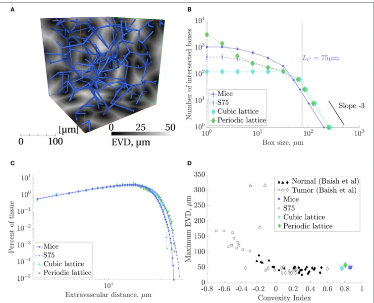
2.3.1. Space-Filling Nature of Capillary Networks A key feature of cerebral capillary architecture that we wish to replicate in the synthetic networks is that they are homogeneous i.e., space-filling at scales above a cut-off length of 25–75µm (Lorthois and Cassot, 2010). In contrast, arterioles and venules are quasi-fractal and scale-invariant (Cassot et al., 2009; Lorthois and Cassot, 2010). Following (Lorthois and Cassot, 2010), the non-fractal, space-filling nature of the capillary networks in all ROIs was tested via a multiscale box-counting analysis of the local maxima of extravascular distances (EVDs), seeAppendix A.1.

Additional metrics were extracted from the EVDs, starting with the mean EVD and the mean of the local maxima, i.e., the mean of EVD values computed for all local maxima. The EVD is also related to mass transfer properties, which are strongly dependent on the local spatial arrangement of the capillaries, among other factors (see section 2.3.5). Indeed,Baish et al. (2011) showed that both the maximum EVD and the “convexity index”

reveal distinct properties for tumor vs. healthy networks. The convexity index was defined as the slope of a linear fit to the log-log scale histogram of EVDs at small scales (Appendix A.1).

Baish et al. showed that the maximum EVD was inversely (non- linearly) correlated to the convexity index. Here, both metrics were calculated.

2.3.2. Morphometrical Metrics

The following metrics were computed to quantitatively compare the morphometrical properties of networks:

1. Distribution, mean and SD of vessel lengths, 2. Edge density (number of vessels per volume), 3. Length density (sum of vessel lengths per volume),

4. Interior vertex density (number of non-boundary vertices per volume),

5. Boundary vertex density (number of boundary vertices per surface area of the region of interest).

2.3.3. Topological Metrics

For a simple topological metric, the percentage of interior vertices with more than three connections was calculated.

For a more thorough quantitative assessment, an algorithm to identify the shortest loops in a network was developed.

The shortest loops associated with each vertexviwere defined as the set of closed loops starting at vi that also pass through neighboring connected verticesv^neigh_j andv^neigh_k , for all values of j = 1,. . .,nandk = 1,. . .,n, k 6= j, wherenis the number of neighboring vertices. The procedure for identifying capillary loops is illustrated inFigure 3A. Identifying the neighbor vertices 2, 3, and 5 directly connected to the root vertex 1, each of the three possible pairs of these vertices was considered in turn.

The shortest path between each pair of vertices without passing through the root vertex was computed using Dijkstra’s algorithm.

Here, each edge was assumed to have unit weight for simplicity, but in practice edges were weighted by their length. The shortest path between vertices 3 and 5 without passing through vertex 1 is 3-4-5. This path was then added to the edges linking vertices 3 and 5 with the root vertex to obtain the final loop path 1-3- 4-5-1. For this “root vertex,” two other loops, 1-5-7-6-2-1 and 1-2-8-3-1, were also found. For each root vertex, there are a maximum ofC2(n) loops, wherenis normally 3. However, each loop was identified multiple times (once for each vertex in the loop) and repetitions were identified and deleted. Selected loops identified in a synthetic network are shown in Figure 3B. The mean number of edges per loop, mean total loop length and mean number of loops per edge were calculated for all networks.

2.3.4. Flow Metrics

As discussed in section 2.2.1, for simplicity, uniform vessel diameters of 5µm were assigned in all ROIs for the purpose of blood flow simulations. Flow solutions were computed using

FIGURE 3 | (A)Schematic illustration of a section of network containing three capillary loops (identified in red, green, and blue) centered around a “root vertex” labeled1.(B)Four individual loops (in thick red) identified in a synthetic network (in dark blue).

an in-house 1D network flow solver (Peyrounette et al., 2018), which takes a classical network approach i.e., assumes a linear relationship between flow and pressure drop in vessels, and conservation of flow at vertices (Appendix A.2). For brevity, all flow results are presented for a pressure gradient in the x-direction only.

The velocity in each capillary was calculated by dividing the flowrate by the vessel cross-section, and the mean and SD of velocities in each ROI was computed.

Next, the permeability was computed. This effective parameter captures the capacity for blood to flow through a representative portion of the network. If divided by the effective viscosity, it is sometimes referred to as the network conductance (Smith et al., 2014; El-Bouri and Payne, 2015). Following (Reichold et al., 2009), the permeability was calculated by applying a pressure gradient across the ROI. By analogy with the theoretical value obtained by applying volume-averaging/homogenization techniques to derive Darcy flow (Smith et al., 2014), the permeability is then given by:

Kx= µ 1Px/Lx

Qx

Ax

, (1)

whereKx,1Px, andLxare the permeability, pressure drop and length of the domain, respectively, in thex-direction.Qxis the corresponding global flowrate, defined as the sum of the flows entering the domain through the face perpendicular to thex- direction, andAx is the area of this face. Because all diameters are uniform, the effective viscosityµis simply the viscosity in all vessels. Note that in contrast to the velocity, the permeability is independent of the magnitude of1P.

2.3.5. Mass Transfer Metrics

Firstly, the transit time (i.e., the time spent by blood traversing each capillary) was calculated as the vessel length divided by the mean vessel velocity, to yield the distribution of transit times, and the median transit time was recorded.

Secondly, in a similar way to the permeability calculation, averaging techniques were employed to derive a macro-scale effective parameterh, known as the mass exchange coefficient (Whitaker, 1999). For details of this method seeAppendix A.3.

This coefficient captures the network-specific capability for mass transfer between the capillaries and the surrounding tissue.

The value ofh characterizes the network architecture and the diffusion properties of both blood and tissue. Here, we consider the diffusion of a non-reactive, non-metabolic tracer, which is highly diffusible through the blood brain barrier. Under these assumptions, and for space-filling networks,his correlated with the surface area available for mass exchange and hence also with the vessel length density, given the uniform distribution of diameters assigned here. The mass exchange coefficienth is reported for a ratio of tissue to vessel diffusion coefficients of 0.25 (Appendix A.3).

2.3.6. Robustness to Occlusions

The robustness of the capillary networks to occlusions was quantified by applying a single occlusion in turn to each edge upstream of a three-connected vertex. Numerically, occlusions

A B

8

were imposed via a diameter reduction factor of 100 in the occluded edge (Cruz Hernández et al., 2019). Because of their different behavior, converging (two inflows, one outflow) and diverging (one inflow, two outflows) vertices were considered separately as inNishimura et al. (2006). The ratio of post- to pre- occlusion flowrates in the outflow edge(s) was computed, with the criterion that baseline i.e., pre-occlusion absolute flowrates in all inflow and outflow edges were greater than a specified tolerance (qtol =0.001% of the total inflow), otherwise the edge was ignored. The final metric reported was the mean of these flow ratios for each case, averaged over all ROIs.

3. RESULTS

In this section, we first assess the architecture of mice and humans capillary networks using the simplest morphometrical and topological metrics. As wee shall see in section 3.1, the results suggest that rescaling is needed to accurately compare capillary networks between species. This implies that the characteristic lengthLCof the synthetic networks developed here needs to be independently chosen for both species. To guide this choice, we study their scaling properties, as well as those of the simpler grid- like networks, as a function of domain size and LC in section 3.2. Finally, the structure and function of these networks with

LC=75µm andLC=95µm is compared to those of the mouse and human data in sections 3.3 and 3.4, respectively.

3.1. A Simple Re-scaling Accounts for Inter-species Differences in Anatomical Networks

A preliminary comparison between the mouse and human anatomical networks was conducted using the simplest morphometric metrics (Table 1, Table S1). These showed that capillaries in the human ROIs were longer (mean capillary length 34.4% higher) and spaced further apart (mean EVD 15.8% higher) than in mice. Nonetheless, loop metrics were very similar, with the mean number of edges per loop almost identical between species. The histograms of this metric were also similar, although with more variance for humans (Figure 4A) suggesting that this distribution was not statistically converged withN =4 samples (compared toN =7 for mice).

Thus, the underlying topology of the networks is comparable but the scaling of the human network is increased relative to the mouse.

This hypothesis was supported by down-scaling the human capillary lengths by the cross-species difference in mean lengths.

The rescaled length histograms for humans (red dashed lines in

TABLE 1 |The geometrical, topological and functional metrics calculated here, for mice, synthetic withL_C=75µm (“S75”), and lattice ROIs.

Metric Mice S75 Periodic Lattice Cubic Lattice

N 7 10 1 1

Mean EVD (µm) 18.4±0.9 20.2±0.6 18.9 19.3

Mean local max EVD (µm) 29.4±1.5 34.5±1.4 36.0 47.4

Max EVD (µm) 50.1±3.7 53.4±2.6 57.3 47.4

Convexity index 0.9±0.1 0.9±0.0 0.8 0.8

Mean length (µm) 44.8±2.4 36.0±1.5 41.0 67.0

SD length (µm) 28.1±2.3 18.5±1.5 0.0 0.0

Edge density (10³mm⁻³) 17.0±1.4 21.3±0.8 17.7 12.5

Length density (mm⁻²) 673±58 674±20 661 668

Vertex density (10³mm⁻³) 8.2±0.6 11.4±0.4 10.7 3.3

Boundary vertex density (mm⁻²) 351±46 317±23 132 223

% multiply-connected vertices 7.2±0.9 2.2±1.0 0.0 100.0

Mean no. edge/loop 11.2±1.2 10.3±0.6 9.0 5.1

Mean loop length (µm) 486±60 368±35 369 345

Mean no. loop/edge 5.1±0.3 4.9±0.4 4.0 9.0

Mean velocity (µm/s) 197±43 204±29 286 268

SD velocity (µm/s) 258±31 233±18 273 380

Permeability (10⁻³µm²) 1.57±0.38 1.38±0.26 2.03 3.42

Median transit time (s) 0.14±0.04 0.13±0.02 0.10 0.08

Exchange coefficienth 24.9±3.31 21.3±0.83 31.5 33.1

Post-occlusion flow ratio (converging) 0.77±0.01 0.76±0.01 0.69 -

Post-occlusion flow ratio (diverging; branch A) 0.26±0.03 0.29±0.02 0.07 -

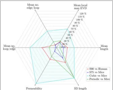
Results are presented as mean±S.D. over the N ROIs studied for each network type (i.e., for the metric “Mean length,” the mean length was calculated for each ROI, and the mean and S.D. of these mean lengths over all ROIs are presented in the table). Colors indicate values that are within 10% (green), more than 10% lower (blue) or more than 10% higher (red) than the corresponding values for the mice ROIs. Permeabilities, velocities and transit times were calculated with uniform diameters of 5µm. Some key metrics are represented (as percentage errors relative to values for the mice data) inFigure 10.

FIGURE 4 |Histograms of(A)number of edges per loop, and(B)capillary lengths on a log-scale, in mouse and human ROIs. The human length distribution rescaled to match the mean length for mice is superimposed in dashed lines. For all plots, frequencies were collected over all ROIs for each species. Error bars show the SD between ROIs.

Figure 4B), coincided closely with the histogram for mice. Thus, we hypothesize that the synthetic networks developed here can be generated to model either mouse or human cerebral capillary networks by an appropriate choice of characteristic lengthLCfor each species.

3.2. Scaling and Convergence of Metrics in Synthetic Networks

Metrics characterizing the architectural, flow and transport properties of porous or heterogeneous media usually vary with the size of the domain under study until a characteristic size is reached, known as a Representative Elementary Volume (REV) (Bear, 1988). Above this REV size, the medium can be considered homogeneous and finite-size effects become negligible. Here, convergence of properties of the synthetic networks with domain size is first studied to determine their REV. This enables overcoming the difficulty associated to anatomical datasets, where both arterioles/venules and capillaries are intermingled, which makes it only possible to extract capillary regions of limited size, may be smaller than the REV. The scaling properties of the synthetic networks withLC are then investigated. For that purpose, some metrics were normalized by an appropriate power of LC, guided by the derivation of analytical expressions for these metrics in the lattice networks, which was possible thanks to their simple architecture. As detailed in section S2.1 of the Supplementary Material, the mean loop length, length density, and permeability scaled with LC, 1/L²_C, and ^d4

L²_C, respectively, wheredis the vessel diameter.

3.2.1. Convergence of Metrics With Domain Size The convergence of metrics in the synthetic networks was studied for domain sizes fromL³_Cto (9LC)³, with metrics normalized by the appropriate power ofLC(Figure 5).

The convergence of metrics was defined as:

M^k−M^k−1

M^k , (2)

whereM^kis the value of the metric in question at sizek. Each metric was considered converged once this value was<0.05. The convergence plots of loop metric with domain size are shown in the insets ofFigure 5andFigure S4. Loop metrics in particular were highly sensitive to finite-size effects, as expected from the analytical results obtained in the lattice networks (section S2.1). For example, the number of loops per edge was higher in vessels nearer the center of the domain than near the boundary (Figure 9Ain Results), explaining the dependence of this metric on domain size.

The mean length, mean number of edges per loop and mean number of loops per edge all converged for domain sizes between (3LC)³ and (4LC)³. This is much faster than in the lattice networks (Figure S2), suggesting that the introduction of randomness to network structures reduces the sensitivity of loop metrics to finite-size effects. By contrast, the permeability converged slower, by sizes of (5.5LC)³.

This is slower than the results recently presented by our group (Peyrounette et al., 2018), where a range of network sizes were obtained by extracting sub-regions from the largest network studied; in contrast, here networks were stochastically re-generated independently for each size, leading to more variance. Interestingly, the permeability converged immediately in the lattice networks (section S2.1), showing that simple lattice networks cannot be used as an analogy to define appropriate REV sizes for more disordered Voronoi-like networks.

In these networks, for all the considered metrics to converge to within 5%, the domain size should be at least (5.5LC)³, which defines the size of the REV.

Above, e.g., with a domain size of (9LC)³, the mean vessel length converged to 0.49LC, while the mean number of edges per loop and loops per edge converged to 9.9 and 5.7, respectively.

A 40 35

00 30

p..

] 25 'B 20

1:l 8 15

'-' Cl)

0... 10

5

5 10 15 20

Number of edges per loop + Mice + Human

25 30

B 25 r ~ - - - , + Mice

+ Human

CfJ 20 -I -Human (rescaled) fili

as

4-<

0

§

u '-'

Cl)

0...

5

Length, µm

FIGURE 5 |Convergence of metrics with domain size in the synthetic networks:(A)mean length,(B)mean number of loops per edge,(C)mean number of edges per loop,(D)mean permeability. Metrics were normalized by the appropriate power ofLC. Insets: the convergence of each metric as defined in Equation (2). The converged sizexconvis the size from which the convergence was<0.05.

The mean permeability converged to 10.4/L²_Cµm⁴with vessels of diameter 5µm, or 0.017d⁴/L²_C.

3.2.2. Scaling With Characteristic LengthL_C

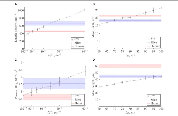
The scaling of metrics was studied forLC between 60µm and 100µm, with fixed domain size (240µm)³corresponding to the size of the mouse ROIs (Figure 6,Figure S5). As expected from the lattice networks (section S2.1), mean capillary length, mean EVD and mean loop length were linearly proportional to LC, while length density and permeability both scaled with 1/L²_C. For reference, linear fits to these graphs are given inTable S2. The mean number of edges per loop did not change withLCfor the range of values considered (Figure S5c), which is not surprising since this is a purely topological metric.

We chose to derive appropriate values ofLCby matching the length densities in the synthetic networks and the anatomical data. Since uniform diameters were imposed in all networks, the length density is linearly proportional to both the porosity i.e., volume fraction of the domain occupied by vessels, which

is important for the flow properties of the network, and also to the vessel surface area per volume, which is a key determinant of mass transfer properties. To best match the mean length density in the mouse ROIs, we chose LC = 75µm, while for humans we set LC = 90µm (Figure 6A).

By matching length density, we obtain a compromise between matching mean length and mean loop length, which were too low, and the mean EVD and edge density which were too high. With these choices of LC, the mean permeability was lower than mice and higher than humans, but nonetheless fell within or just outside the error bands for both species.

The SD was particularly high for the permeability and of the same order for synthetic and anatomical networks (Figures 6C).

Since this study was conducted with variable LC at a fixed domain size, the number of unit cells decreases with increasing LC, possibly introducing finite-size effects. In the range considered, the number of cells varied from 4³withLC=60µm to 2.4³withLC =100µm. The decrease in the mean number of

A 0.5

(.)

~ --...

..c: _--0 :

_§

,:; ro

<l)

:;s

0 1

C 12

P-. 10

0

.::::::. 0 8

<l)

bO

"O

<l)

0 6

,:;

,:; 4

ro <l)

~ 2

0 1

t __ ^{-f--f---i- -+-}

' -- --f

: : 2

2

3 4

~ 0.8

al 0.6 ::.0

~ 0.4

"

8 0.2 \

0 t:±::Z:::S:;;;;;;;=====

! ^Xconv = 3.5Le

5

2 3 4 5 6 7 8 9 Network side length / Le

6 ⁷ 8 9

Network side length / Le

3 4

~ 0 4 .

~ O 2 ^·Xconv = 3Le

0

5

2 3 4 5 6 7 8 9 Network side length / Le

6 7 8

Network side length / Le

9 B

<l)

bO

"O

6 5

~4

P-. 0

..S3

0 ,:;

~ 2

<l)

~

J-,t'--f- yf +·I·+~.+-~

t1i\

8

2 3 4 5 6 7 8 9 Network side length / Le

o~~~-~--~-~-~--~-~-~

1

D 11

"'s

::i. 9

M

I 8

0 r-<

c-,\.) 7

....;i 6

X

>, 5

~ 4

ii _ro

<l) 3

s

<l)

0... 1 0

1

2 3 4 5 6 7 8 9

Network side length / Le

' __ I+++H. ~ , +-t-++•·+fl

r

'

:

~ 0.4

" \

8 0.2 ^Xcmw = 5.5Le

2 3 4 5

ot=:::::::-"'==::=s:;;;;;===

2 3 4 5 6 7 8 9 Network side length / Le

6 7 8

Network side length / Le

9

FIGURE 6 |Scaling of metrics with the characteristic lengthL_Cin the synthetic networks:(A)length density,(B)mean EVD,(C)permeability,(D)mean length.

Errorbars show mean±S.D. for the synthetic networks. Shaded bands in blue and red show mean±S.D. of mouse and human values, respectively.

loops per edge as a function ofLC(Figure S5d) demonstrates this effect: as shown in the previous section, this metric converges from 4³unit cells, and does not depend onLCfor larger domain sizes. Nonetheless, the length density converged very quickly with domain size, for 2³ unit cells or more (Figure S4b), thus the choice ofLC via the length density was unaffected by finite-size effects. Finite-size effects also had a small influence on the linear fits shown inTable S2; if keeping the number of cells fixed to e.g., 3³, a maximum difference of approximately 14% was found in the predicted slope.

Final synthetic networks were thus generated in the same domain sizes as the corresponding anatomical ROIs. Synthetic networks matched to the mouse data had domain size (240µm)³; with LC = 75µm, this size is equivalent to (3.2LC)³, or (0.58)³× the REV size. The error in the calculated metrics due to the finite domain size was estimated using the previous convergence study. For example, the number of edges per loop converged quickly with increasing domain size, and, in the ROI sizes studied, was predicted to deviate only 4% from the converged value. However, the predicted permeability with ROIs of (240µm)³was expected to be approximately 25% lower than its converged value. REV sizes and corresponding convergence trends could not be determined for the anatomical datasets, due to the limited size of capillary ROIs. However if we assume that

metrics converge in a similar way, similar finite-size related errors can be expected.

Similar to the synthetic networks, the lattice networks were scaled to match the mean length density in the anatomical networks, to minimize any differences due to scaling. However, as lattice networks did not have equivalent properties either to mice or humans, results for the lattice networks scaled to match the mouse data only are presented in section S2 of the Supplementary Material.

3.3. Synthetic Networks With L

= 75µm Effectively Replicate Mouse Capillary Networks

Metrics computed for synthetic networks with LC = 75µm and domain size (240µm)³were compared to their values in the mouse networks. The mean and SD across all ROIs of all metrics are listed inTable 1.

3.3.1. Space-Filling Metrics: Synthetic Networks Have Equivalent Space-Filling Properties as Mice ROIs Slices of the EVD map with the corresponding synthetic network superimposed are shown inFigure 7A. Applying box- counting methods to the local maxima of EVDs confirmed the

A

1000

N

I

a

a

;,:;

_.., 600

·.;

Q

<l)

"O ..c:: _.., 400

bJl Q

<l)

.-a 200

---f----

_,r - + _--+-- ^---t--

,-l

1--

~~~I

-,-S75

···Mice

···Human

0 L__.__ _ __._ _ _ _ __._ _ _

--====-,

100-² 90-² 30-² 70-² 60-²

L" c/ ,

C 3

N 2.5

J

0 ...

~ 1.5 1--- - - --+-~--+- - - -

1

f f---+---+---- -

a --

... --

<l)

P... 0.5 + S75

•···Mice

···Human

0L__.__ _ __,_ _ _ _ _ ,__ _

_':===

100-² 90-² 30-² 70-² 60-²

L e/,

B

-+----+---+

•• I---- - - - 25

a

-+--- -+--

::i.. 1--- -~

Q ---+--

>

r.,:i Q

~ 10

~

5 -i-S75

•···Mice

···Human

0 L___, _ __,_ _ __._ _ __._ _ _,_ _

_._:===

60 65 70 75 80 85 90 95 100

Le, µm D

60 8 50

i:

^{-r -- - __ - _}

^{- - -+ ~ - - - - ~ --· faa••·}

~ ~ 20

+ S75

•···Mice

10

···Human

0 L _ _ . . _ _ _ _,___-'----'---'---...:====

60 65 70 75 80 85 90 95 100

Le, µm