Publisher’s version / Version de l'éditeur:
Journal of Water, Air and Soil Pollution, 143, 1-4, pp. 41-63, 2003-01-01
READ THESE TERMS AND CONDITIONS CAREFULLY BEFORE USING THIS WEBSITE. https://nrc-publications.canada.ca/eng/copyright
Vous avez des questions? Nous pouvons vous aider. Pour communiquer directement avec un auteur, consultez la première page de la revue dans laquelle son article a été publié afin de trouver ses coordonnées. Si vous n’arrivez pas à les repérer, communiquez avec nous à PublicationsArchive-ArchivesPublications@nrc-cnrc.gc.ca.
Questions? Contact the NRC Publications Archive team at
PublicationsArchive-ArchivesPublications@nrc-cnrc.gc.ca. If you wish to email the authors directly, please see the first page of the publication for their contact information.
NRC Publications Archive
Archives des publications du CNRC
This publication could be one of several versions: author’s original, accepted manuscript or the publisher’s version. / La version de cette publication peut être l’une des suivantes : la version prépublication de l’auteur, la version acceptée du manuscrit ou la version de l’éditeur.
Access and use of this website and the material on it are subject to the Terms and Conditions set forth at Secondary effluent treatment by slow sand filters: performance and risk analysis
Sadiq, R.; Husain, T.; Al-Zahrani, A. M.; Sheikh, A. K.; Farooq, S.
https://publications-cnrc.canada.ca/fra/droits
L’accès à ce site Web et l’utilisation de son contenu sont assujettis aux conditions présentées dans le site LISEZ CES CONDITIONS ATTENTIVEMENT AVANT D’UTILISER CE SITE WEB.
NRC Publications Record / Notice d'Archives des publications de CNRC:
https://nrc-publications.canada.ca/eng/view/object/?id=3e70f00c-0dd8-4177-8d1c-eb35ba58e24f https://publications-cnrc.canada.ca/fra/voir/objet/?id=3e70f00c-0dd8-4177-8d1c-eb35ba58e24f
Se c onda ry e fflue nt t re a t m e nt by slow sa nd filt e rs: pe rform a nc e a nd risk a na lysis
N R C C - 4 5 3 7 8
S a d i q , R . ; H u s a i n , T . ; A l - Z a h r a n i , A . M . ; S h e i k h , A . K . ; F a r o o q , S .J a n u a r y 2 0 0 3
A version of this document is published in / Une version de ce document se trouve dans:
Journal of Water, Air and Soil Pollution, 143, (1-4), pp. 41-63, January 01, 2003
The material in this document is covered by the provisions of the Copyright Act, by Canadian laws, policies, regulations and international agreements. Such provisions serve to identify the information source and, in specific instances, to prohibit reproduction of materials without written permission. For more information visit http://laws.justice.gc.ca/en/showtdm/cs/C-42
Les renseignements dans ce document sont protégés par la Loi sur le droit d'auteur, par les lois, les politiques et les règlements du Canada et des accords internationaux. Ces dispositions permettent d'identifier la source de l'information et, dans certains cas, d'interdire la copie de documents sans permission écrite. Pour obtenir de plus amples renseignements : http://lois.justice.gc.ca/fr/showtdm/cs/C-42
er', Geochim. ing',Environ.
PERFORMANCE AND RISK ANALYSIS
REHAN SADIQh, TAHIR HUSAIN2,A, M, AL-ZAHRANI3,
ANWAR KHALIL SHEIKH4andSHAUKAT FAROOQ3
1Institute for Research in Construction (IRC), National Research Council (NRC), Ottawa, Ontario, Canada; 2Faculty of Engineering and Applied Science, Memorial University of Newfoundland,
St, John's, Newfoundland, Canada; 3Civil Engineering Department, King Fahd University of Petroleum and Minerals, Dhahran, Saudi Arabia;4Mechanical Engineering Department, King
Fahd University of Petroleum and Minerals, Dhahran, Saudi Arabia (* author for correspondence, e-mail: rehan,sadiq@nre,ea,fax: +1-613-954-5984)
(Received 16 August 200 I; accepted 4 June 2002)
Abstract. The objective of this study is to examine the reuse of wastewater for beneficial purposes,
To accomplish this objective, the efficiency of slow sand filters in removing total coliforms(TC) was
studied using a probabilistic method, Three pilot scale slow sand filters were constructed at Alkhobar wastewater treatment plant, Dhahran, Saudi Arabia, The removal efficiency of filters was estimated
under different operating control parameters, which included filtration rate (q), sand bed depth (d)
and sand grain size (c), The Type III extreme value distribution best fitted the removal efficiency
data, A multiple linear regression analysis was performed to develop a relationship for mean removal efficiency as a function of control parameters, The predicted mean response and experimental results of previous studies were compared to validate the empirical regression model. The control paramet-ers and influent concentrations of total coliform were used in Monte Carlo (MC) simulations for calculating the reliability index ({J), The reliability index and corresponding risk were calculated for lognormally distributed safety margins (SM), An effluent standard of 100 total coliform/lOa mL was defined as capacity of the filter to ascertain the risks of exceedence, which was approximately less than 50 for 95% of the time, Pre and/or post disinfection would be necessary to meet the stipulated effluent standards for unrestricted agriculture use,
Keywords: agriculture reuse, Monte Carlo (MC) simulations, multiple linear regression, reliability
index, safety margin, slow sand filters, tertiary treatment, Type III extreme value distribution .
List of symbols <p-l [Fy (Y)] BOD C
r
Jk fJ (J••
Gamma function MeanScale factor for Type III distribution Standard deviation
Transformation factor (NORMSINV in Excel-7) = Z-score Biochemical Oxygen Demand
Capacity (standard of 100 TC/lOO mL) Water, Air, and Soil Pollution 143: 41-63,2003,
e Sand grain size (mm) in I
COY Coefficient of variation (a //L) (W
CDF Cumulative distribution function am
COD Chemical Oxygen Demand pre
d Depth of sand bed (cm) nat
Ei Effluent concentration (TC/lOO mL) bet
FC Fecal Coliform ave
F F -statistics abl
Fy (Y) Cumulative distribution function the
(AI
GoF Goodness of fit of
Ii Influent concentration (TC/lOO mL) Slg
L Load (effluent concentration of TC/IOO mL) rna
m Shape factor for Type III distribution In'
MC Monte Carlo simulation saf
on
MPN Most Probable Number is t
n Number of simulation of
N Total number of data points COl
P Probability of exceedence
of PDF Probability Density Function
Ah
q Flow rate (L min-I), filtration rate (m hr-I) ass
R Random number
fJ
Reliability index spcLog normal scatter factor the
s
SM Safety Margin palres
TC Total Coliform egl
TSS Total Suspended Solids Ur
Xi Risk or reliability index COl
Yo Median value of removal efficiency (%) an,
we
Yi or Y Removal efficiency (%)
Yrn Maximum value of removal efficiency (%) hal
Ymean Mean value of removal efficiency (%) istl
an, ag
l. Introduction en
1'01
Although slow sand filters are in use for water treatment from more than 150 yr, St8 its application in wastewater treatment has recently gained popularity, especially su:
an 150 yr, especially
t
in the context of wastewater reuse (Sadiq, 1997). The World Health Organization (WHO, 1989) guidelines on wastewater reuse in agriculture provide background and guidance to governments for making risk management decisions related to the protection of public health and preservation of environment.
The Kingdom of Saudi Arabia, an arid country, lacks perennial rivers. The national water demand in Saudi Arabia increased from 2.36 to 16.23 x 10⁹ m3
between 1980 and 1990 (Husain and Ahmed, 1997). Due to low rainfall (on an average less than 100 mm yr-I) and the absence of rivers and lakes, the renew-able surface and groundwater resources in Saudi Arabia are not enough to meet the growing demands of domestic, commercial, industrial, and agricultural sectors (Abu Rizaiza and Allam, 1989; AI-Ibrahim, 1990). Groundwater is the main source of water and therefore as a result of high rate of extraction, aquifers are showing significant decline in the water level. Since wastewater reuse can meet these de-mands to a certain extent, the policy is to utilize all treated municipal wastewater in the most beneficial manner with its main use in agricultural sector. In order to safeguard the public health and to protect the environment, regulations are imposed on the reuse of treated wastewater. One of the viable options to treat wastewater is the use of slow sand filters. The main objective of this article is to evaluate risk of total coliform exceedence in slow sand filter effluent under various operating conditions.
Health hazards are associated with the reuse of treated effluents due to presence of waterborne pathogens and chemicals in the reclaimed wastewater (Husain and Ahmed, 1997). The objective of slow sand filtration is to reduce the health risks associated with wastewater and reuse for irrigation and groundwater recharge.
Total coliforms (TC) and fecal coliforms (FC) are used in conjunction with specified requirements for treating wastewater, and in such cases it is assumed that the need for expensive and time consuming monitoring of treated wastewater for pathogenic organisms is eliminated. Bartone (1990) has suggested a guideline for restricted wastewater irrigation based on an effluent with less than one nematode egg/L and Fe of1000/100mL. The World Health Organization (WHO, 1989) and United States Environmental Protection Agency (U.S. EPA, 1980) have also re-commended these guidelines. Numerous technical and policy options for reducing and controlling the health risks associated with the wastewater reuse in agriculture were also evaluated by the UNDPlWorld Bank (Shuval et al., 1986; Shuval, 1987). In recognition of the importance of conserving water resources, Saudi Arabia had planned to recycle 730 x 106 m3 wastewater by the end of year 2000. Min-istry of Agriculture and Water (MAW) Saudi Arabia is responsible for planning and development of all water resources. It is a key organization for implementing agricultural and water-based policies. The MAW in cooperation with other gov-ernmental agencies has established guidelines defining the acceptable standards for wastewater treatment, disposal and reuse. The MAW has promulgated effluent standards of less than 10 mg L-I for biochemical oxygen demand (BOD), total suspended solids (TSS) and N03-N concentrations for agriculture use. In the case
2. Data Collection v Ii o s o o tl d o s u v n t, o tl S 11 ti of FC, a 7-day average of 2.2 most probable number (MPN) per 100 mL (with no
sample more than 100 MPN/IOO mL) for unrestricted irrigation is recommended.
For restricted irrigation, the MAW recommended maximum FC concentration in anyone sample should not exceed 200 MPNIlOO mL and the last 7 days average should be less than 23 MPNIlOO mL. Standards adopted by the MAW are based on the State of California Wastewater Reclamation Criteria (1978).
Meteorology and Environmental Protection Administration (MEPA) Saudi Ar-abia is responsible of environmental surveys and pollution assessment of envir-onmental standards and regulations. The national wastewater discharge regulations are put forward by the MEPA (unpublished report). The MEPA water quality stand-ards were promulgated in order to: minimize the volume of waste generated; reduce discharge of pollutants at source to minimum; ensure maximum assimilation of pollutants; protect the quality of ambient water bodies; and control the quality of wastewater before discharge. In the case of TC, a 7 day average of 2.2 most probable number (MPN) per 100 mL for unrestricted irrigation is recommended. MEPA set a maximum contaminant level (MCL) of 100 MPNIlOO mL TC for unrestricted irrigation and 1000 MPNIlOO mL for discharge into receiving water bodies.
TC includes all types of FC and other non-fecal lactose fermenting, gram-negative bacilli. As an indicator system, the TC group, thereby, contributes a factor of safety beyond that achievable with FC alone. The current study employed wa-ter quality reuse standards of 100 TC/IOO mL for unrestricted irrigation in the
evaluation of slow sand filter treatment efficiency.
Three pilot plant slow sand filters were built at Alkhobar wastewater treatment plant to study the reduction of total coliform population. The quality of secondary wastewater from the treatment plant was measured by taking three replicate grab samples of BOD, chemical oxygen demand (COD), TSS, nitrogen and phosphor-ous (N and P) and microbial indicators. The ranges and average values of the characteristics of the secondary effluent used as the influents for slow sand filter are reported in Table 1. The total coliform concentration ranged from 3.1 x 10³ to 1.2 X 1071100 mL.
Three slow sand filters each of 2 m in diameter were operated for approximately 15 months. Two filters were operated with coarse sand of 0.5 mm effective grain size and one filter with fine sand of 0.3 mm grain size (Farooq and Nakhla, 1996; Khan, 1996; Sadiq, 1997). The filters were operated to investigate the effectiveness of various control variables on the removal efficiency of the microbiological indic-ators. The filters were operated at flow rates of 8, 10, 16 and 20 L min-1 (0.15, 0.20, 0.30 and 0.40 m hr-I) whereas the sand bed depth was varied from 150 to 80 em and then to 50 em. The effect of third control variable i.e. sand grain size
" (with no mmended. ltration in (S average 3based on Saudi Ar-: of envir-egulations lity stand-ed; reduce lilation of he quality '2.2 most nmended. lL TC for ring water ng, gram-es a factor toyed wa-ion in the treatment secondary icate grab phosphor-les of the sand filter lx103to 'Oximately ;tive grain hla, 1996; ectiveness ical indic-n-I (0.15, Jm 150 to grain size TABLE I
Characteristics of secondary effluent from AI-Khobar trealment plant
Parameter Minimum Maximum Average
Temperature (C) 10 39 28 Turbidity (NTU) 0.2 0.95 0.7 BOD (mg L-I) 2.8 6.1 4.8 COD (mg L-I) 32 57.6 41 TSS (mg L-I) 8 88.4 14.7 TKN' (mg L-I) 0 6.2 3.2 Total-P04 (mg L-1) 0 1.15 0.56
Total Coliform (MPN/100 mL) 3.1 E+03 1.2 E+07 3.69 E+05
Fecal Coliform (MPN/IOO mL) O.OE+OO 9.4E+05 1.53 E+05
• TKN: Total Kjeldahl nitrogen.
was studied at two levels - 0.3 mm (fine) and 0.5 mm (coarse). Two filters were filled with 0.5 mm and one filter with 0.3 mm sand grain size. The entire operation of the filter consisted of 14 sets of operating conditions, out of which 5 with fine sand and remaining 9 with coarse sand. The initial four conditions corresponded to operation at 0.5 mm, the next five with 0.3 mm, and the last five conditions were operated at 0.5 mm sand grain size. The program of operation was designed so that when one condition was over, the filter was adjusted to a new operating con-dition with respect to sand bed depth, filtration rate and media grain size. The data were collected under steady state condition upon the development of biological layer (Farooq and Nakhla, 1996; Sadiq, 1997). A summary of operational details is shown in Table
II.
The operation was suspended for some periods because of operational and maintenance problems such as pump failure, etc.Filtration rate control is the key element in operation of filters. For treatment of surface water, generally a filtration rate of 0.1 to 0.2 m hr-I is recommended but up to 0.6 m hr-t is reported in the literature (Visscher, 1988). In this study control valves were used to maintain the flow rate from 0.15 to OAO m hr- I and vigilant monitoring on a daily basis helped in maintaining the desired flow rates. The cri-teria used for terminating filter runs were break through of turbidity or attainment of head loss of 150-175 cm. The desired flow rates could not be maintained over these head losses.
3. Removal Efficiency Modeling
Several mathematical filtration models have been proposed during the last 30 yr. Most of these models were originally developed to describe aerosol removal by fibrous filter and later applied to aquasols (Sadiq, 1997). In filtration mechanisms,
TABLE II
Operating conditions of slow sand tilters
Conditions Grain size Filtration rate Sand bed depth Days of operation Dist
(c) (q) (d) active/inactive (mm) (L min-I) (mhr- I) (em) Non 1 0.5 8 0.15 150 177/32 2 0.5 10 0.20 150 35/1 3 0.5 10 0.20 80 99/2 4 0.5 10 0.20 50 76/2 5 0.3 16 0.30 150 191/39 Log 6 0.3 20 0.40 150 2111 7 0.3 20 0.40 80 99/3 8 0.3 20 0.40 50 79/3 9 0.3 10 0.20 50 18/0 10 0.5 16 0.30 150 191155 11 0.5 20 0.40 150 6011 12 0.5 20 0.40 80 60/2 Typ' 13 0.5 20 0.40 50 79/6 14 0.5 16 0.30 50 18/0 Extr
macroscopic and microscopic theories are widely accepted. In the macroscopic approach, a first order kinetics in the removal of particulate is assumed, whereas the microscopic approach takes into account single collectors efficiencies. Filtration equations describing the deep bed filtration of aquasols were proposed by Yao
et al. (1971). Similarly there are many other models available in the literature
inclUding Hinds (1983), Rubow and Liu (1986), Tien and Paytakes (1976) and Fuchs (1964). These models require data for characteristics of filter media, type of flow and liquid. Contrary to above listed models a statistical approach is employed in this research to model the removal efficiency as a function of operating control parameters.
3.1. SELECTION OF THE DISTRIBUTION
Exponential, normal, lognormal, uniform, weibull and various types of extreme value distributions are commonly used distributions for data fitting. The removal efficiency is calculated by
(I- E)
y.= l l x100 I Ii 1 .__.•.__. _ - - - _
...
;0-1 [ ofsyn where J fluent tl paramel didate c The det: ers (me: summar The dom Val distribul bution i 100%iT; Them iTABLE III
Statistical distributions for removal et1iciency (Raudkivi. 1979: Lewis. 1987) leration tive Distribution Normal Lognormal Linearized form
Jly
=MeanO"y =Standard deviation
Ln(Yi)=Ln(Yo)+scp-l [Fy(Yi)]
Jl2
[Jl
2
+0"2]
Yo = y and s = Ln y 2 Y
Ajャセ
+
oBセ
Jly
Yo =Median
s=Measure of scatter
'1'-1 [Fy (Y)]
=
Z-Score andYi=
Removal efficiency. (See definition of parameters in the list of symbols).where Yio Ii and E; are % removal efficiency, influent total coliform, and ef-fluent total coliform concentrations, respectively. To estimate the characteristic parameters of the distribution, removal efficiency data were fitted to three can-didate distributions: normal, lognormal and extreme value Type III distribution. The details of CDF (cumulative distribution function) and characteristic paramet-ers (mean, median and standard deviation etc.) of the selected distributions are summarized in Table III.
The normal distribution is the most commonly used distribution when the ran-dom variable Y; arises from the sum of a number of random effects. Lognormal distribution is suitable when Y; is a product of random effects. The Type III distri-bution is a three parameter model and has a truncation (Ym) on one side, which is 100% in our case. Them and13are the two unknown parameters of this distribution. The m is the shape factor, which gives information about scatter of data and 13 is Lcroscopic hereas the Filtration d by Yao literature 1976) and ia, type of employed ng control >f extreme e removal
Type III exp [-
em;
YifJ
Extreme value
Ln Ln
(_1_)
mLn(Ym - Yi) - mLn(e)FY(Yi)
JlY Ym-er(1+
セI
0"2
=e
2[r
(1+
セI
-
r
2(I
+
セI
J
Ym =Maximum value m=Shape factore
=Scale factor1.0イMMMMMMLMMMMMMMMMMMMMMMMMMMセMt
...
",. ..-....
-'-
--
---- ---- ----
. .
.
...-.-
...:-...
0.2 0.8 ... --+-COF - - - Normal 0.6 ... ...セ
-Lognormal-
• TypeIII0.4 100 95 90 85 80 75 70 65 60 55 0.0 KMMセMM⦅K⦅MMセMセMMセMMセMセMMセMMゥ⦅M⦅⦅\ 50 Y (R.E.%)
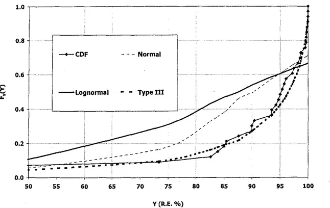
Figure1. CDF of removal efficiency of total coliform. condition 1.
the scale factor. The expected value and variance of the distribution are given in Table III. The details of these distributions can be found elsewhere (Lewis, 1987).
For each condition, a set of data points were obtained (number ranges from 6
to 38) for total coliforms at the influent and the effluent end of filter. The removal efficiency of bacterial indicators through the slow sand filter was fitted to normal, lognormal and Type III maximum extreme value distributions. The Kolmogrov-Simmov (K-S) test was performed to check the goodness of fit (OoF) for candidate distributions. The details of this statistics can be seen elsewhere (Sadiq, 1997; Benjamin, 1970). The empirical CDF of total coliform removal efficiency for con-dition #1 is plotted in Figure 1.The CDFs of all three distributions are also plotted on the same graph. The results of OoF test confirmed that Type III distribution characterized the removal efficiency data in the best manner. The summary of K-S test results is given in Table IV. The result shows that Type III distribution is the best candidate for removal efficiency data in 8 conditions out of 14, which is shown by shaded boxes. Even for remaining operating conditions the values were within 5%level of significance.
The selected distribution was fitted and regressed to the data. The method of least square was used to estimate the parameters of the Type III distribution. The estimated parameters of the distribution were used to calculate mean response, and to develop an empirical model as a function of operating conditions. The equa-tion was linearized to plot the data on the Type III distribuequa-tion (Table III). The characteristic parameters m and
e
were calculated from the intercept and slope ofstraigi axis. 1 plottir where plot f( The al obtain by cor mgm( also re As depen, imply III con condit condit condit
TABLE IV
Summary of K-S test for removal efficiency data
Conditions Data K-S Normal Lognormal Type III"
points (%) 1 33 0.234 0.406 0.287 0.100 2 10 0.410 0.136 0.131 0.158 3 14 0.349 0.353 0.267 0.335 4 17 0.318 0.144 0.147 0.159 5 38 0.221 0.255 0.158 0.132 6 6 0.521 0.212 0.210 0.213 7 14 0.349 0.125 0.126 0.126 8 17 0.318 0.242 0.254 0.257 9 9 0.412 0.230 0.331 0.122 10 38 0.221 0.274 0.302 0.251 95 100 11 14 0.349 0.299 0.307 0.203 12 6 0.521 0.161 0.158 0.151 13 17 0.318 0.199 0.191 0.168 14 9 0.432 0.223 0.219 0.213
a Bold figures showing Type III as the best fit.
straight-line equation by plotting Ln Ln [1/F (Y)] on y-axis and Ln (Ym-Y) on x-axis. The probability positions were calculated by the mean rank formula (Weibull plotting position) as given by the following equation.
where N is the total number of data points and iis the ith observation. The fitted
plot for condition #1 of total coliform removal efficiency is shown in Figure 2. The above procedure was repeated for other conditions and similar results were obtained and these are summarized in TableV. The m and
e
values were calculated by comparing fitted equation with the straight-line equation. The statistics includ-ing mean(Ymean ), standard deviation (O'y) and coefficient of determination (R2) are also reported in Table V.As shown in Table V the extreme value is a skewed distribution and its shape depends on parameter m. The smaller values of m indicate a higher skewness and
imply a higher variability in data. The mean removal value (Ymean)of total coliform
in condition 1 was 96.5% with a standard deviation of 10%. In all operational conditions the removal efficiencies of total coliform were more than 90% except for conditions 4, 8 and 13. The conditions 8 and 13 represented the extreme operational condition with respect to a high flow of 20 L min-I (0.40 m hel) and low bed セ given in is, 1987). es from 6 e removal o normal, Ilmogrov-candidate iq, 1997; ( for con-;0plotted ,tribution ry of K-S on is the is shown re within lethod of :ion. The lllse, and he equa-III). The slope of i Fy(Yj ) = -(N-+-I) , (1)
---
-LnLn(l/Fy)=0.561 x Ln(Ym·Y)· 1.09 2.0 1.0 0.0
;;:.
-
..
-1.0 セ c -J C -J -2.0 -3.0•
-4.0 -3.0 -2.0 -1.0 0.0 1.0 2.0 R2=0.97 3.0 4.0 5.0 depth depth satisf2 Ln(ym·Y)Figure 2. Fit of Type III maximum extreme value distribution to characterize the removal efficiency of total coliform, condition 1.
TABLE V
Removal efficiency data of total coliform at various operational
condi-tions
Conditions Data points R2 m
e
Ymean cry1 33 0.97 0.56 7.00 96.48 10.60 2 10 0.89 2.06 2.96 97.38 1.33 3 14 0.99 4.44 2.72 97.52 0.63 4 17 0.89 4.93 17.51 83.94 3.73 5 38 0.93 0.90 5.49 94.40 5.84 6 6 0.92 1.11 2.49 97.61 2.16 7 14 0.94 2.11 6.31 94.41 2.79 8 17 0.80 4.19 23.00 79.10 5.62 9 9 0.92 4.84 12.32 88.71 2.66 10 38 0.82 1.30 5.44 94.98 3.90 11 14 0.95 1.24 5.93 94.47 4.49 12 6 0.97 2.82 10.00 91.09 3.43 13 17 0.94 5.73 22.44 79.24 4.20 14 9 0.88 6.30 1.15 98.93 0.20 3.2. ] To pre respOl regres filtrati wasSl best r. deterr on va scatte regre, the fa JLI when イ・ァイ・セ from distril the n signi! at apl mode 20L for gl
TABLE VI
Coefficients of regression model
A
•
Predictor Coefficient Standard deviation t-ratio pConstant 108.1 20.57 5.26 0.000 c -85.9 34.46 -2.49 0.037 q -2.58 0.8650 -2.98 0.018 d 0.537 0.2794 1.92 0.091 1.09 d·q·c 0.0585 0.02163 2.70 0.027 d 2 -0.0023 0.001357 -1.70 0.127 5.0 ,1 efficiency
depth of 50 cm. In condition 4, although the flow rate was not high but the bed depth was the minimum. The data fitted well in all conditions and R2 values were satisfactorily high (0.78-0.99).
3.2. REGRESSION MODEL OF AVERAGE REMOVAL EFFICIENCY
To predict the removal efficiency of total coliform through slow sand filters a mean response model as a function of control variables is required. A multiple linear regression model is developed to predict removal efficiency of total coliform using filtration rate (q), sand bed depth(d) and effective media grain size (c). The model was selected based on regression diagnostics. One of the criteria for selection of the best model was to check the significance of independent variables, which can be determined from individual p-values. The selection of a regression model is based on various statistical parameters such as mean absolute error (MAE), leverage, scattering and trend of residuals, R2 and R;dj' overall p-value of model. Several regression models were tried to get statistically acceptable results before selecting the following final regression equation:
!-iy = 108 - 85.9(c) - 2.58(q)
+
0.54(d)+
0.059(d·q·c) - 0.0023(d2) , (2)where !-iy is the mean response of the removal efficiency (Yi ). The diagnostics of regression model is shown in Figure 3. The normality of residuals can be observed from normality plot and histogram, which has the approximate shape of a normal distribution. The homoscedacity and trends of residuals were also studied to ensure the regression assumptions. The coefficients of independent variables and their significance levels are given in Table VI. The individual p-values are significant at approximately 90% or more for all variables. The range for which regression model can predict the mean removal efficiency varies from 0.15 to 0.4 m hr-1(8 to 20 L min-I) for filtration rate, 50 to 150 cm for sand bed depth and 0.3 to 0.5 mm for grain size.
Normal Plot of Residuals Chart of Residuals • -5 1--.----,---..,.---r----,! -2 -1
a
2 Z-Score Histogram of Residuals R E Ts
DF セWNPTQ LQ...·7.04\ セッNッッッ 15 5 10 Observation Number Residuals vs. Fits a -101 - - - - , - - - , - - - , ' 0; :l セ 0 Ql 0: 10-c---.
• • ••• • • ••• • • 5 -0; :l '0 'iii Ql 0-0: -5.0 -2.5 0.0 2.5 5.0 7.5 Residual • 4g
3 Ql :l 2 C" l" u. 1a
r - --I
, 5-0; :l '0 'iii Qla
• 0: • -5 80 • 85 • •...
•• • • • 90 95 FitFigure3. Regression analysis and model diagnostics ofresiduals.
The analysis of variance (ANOVA) of the selected model is given in Table VII. The coefficient of determination (R2 "" 0.76), implied that76.40% of the variability of dependent variable (/-Ly) was explained by this model. TheR;dj value is 61.7%,
which is a more reliable parameter for multiple regression models. The advantage of the R;dj over R2 is that, it does not increase automatically as new regressors are inserted in to the model (Montgomery, 1991). The standard error (4.17) of the estimate is the standard deviation of the residuals. The mean absolute error (MAE) of 2.54 is the average value of the residuals. The calculated F value is 5.18, which gave overall p-value of0.02 giving a significance level of 98%. A comparison of predicted and measured values, and confidence and prediction interval envelopes are plotted in Figure 4.
Pre(
3.3. MODEL VALIDATION
Three studies were selected from literature and values of filtration rate, sand bed depth and media grain size were used to predict the mean response from the model. As shown in Table VIII, a close agreement between experimental results and pre-dicted values is observed. The filtration rate reported in (m hr-1) was converted into (L min-I) correspond:ng to 2 m diameter filterfor using this regression model.
A regression model was used to determine the optimum range of operation for slow sand filters. The contours of removal efficiency at fixed level of sand grain size (c
=
0.3 and 0.5 mm) were plotted and shown in Figures 5 and 6. To achievere-mova from 0.5 m the sa ,hOWl ofvie andd sand 1
,""
OF: Degree of freedom; SS: sum of squares; MS: mean sum of squares; and F: F-test value.
···95.0% Confidence Bands _._.- 95.0% Prediction Bands
Figure4. Comparison of fitted and measured values. "" " Table VII. variability is 61.7%, advantage regressors .17) of the 'or (MAE) .18, which parison of envelopes Predicted 100 90 80 70 80 85 Arflll,,1 90 95 , sand bed the model. sand pre-verted into model. セイ。エゥッョ for grain size .chieve
re-mova1 efficiency of 98% or more for 0.3 mm grain size, the depth(d) should range from 75 to 130 cm and filtration rate (q) from 0.22 to 0.35 m hel. Similarly for 0.5 mm grain size, the range for filtration rate was from 0.19 to 0.36 mhr-1to get the same removal efficiency. The optimum ranges of depths and filtration rates are shown in Figures 5 and 6. These ranges are important from optimal operation point of view. It can be observed from the ranges of optimum operational conditions of q andd that grain size does not affect significantly to the removal efficiency of slow sand filters. The model developed in this section will now be used for risk analysis.
TABLE VIII
Comparison of predicted and experimental results
Study Details Filtration rate q d c Ypredicted Yexperimental
HュィイセャI HlュゥョセャI (cm) (mm)
'"
AI-Yousaf (1990) Pilot-scale 0.16 8.4 55 0.31 90.66 93.46
'"
»diameter= I m 0.16 8.4 105 0.56 98.02 97.26 ,Q0
Bellamyet al. (1985) Pilot-scale 0.12 6.3 48 0.29 92.45 92.00 セ»
diameter=0.3 m 0.12 6.3 97 0.62 90.99 96.50 r
Ellis (1987) Pilot-scale 0.30 15.7 95 0.60 98.48 99.00
diameter=0.14 m 0.15 7.85 95 0.60 92.55 99.00
セア「^GᄋBBGNo\GᄋBB[G
---
l---
セ
1/
L---
l-1/
⦅G⦅BNセGLッイゥBGN
)
fore=0.3nun d =75to130 em//;
q= 11.5to18.5 Llmin (0.22to0.35m1h) 98g
96 94 92 8 10 12 14 q(Umin) 16 18 150 120 100!
." 80 50 20Figure5. Contours of removal efficiency at 0.3 mm sand grain size.
イMMMM]MイMMMMNNNNBNLNMMMMMイMMMMMMMLMMMM]セMMM⦅イQUP
・MMMMMNNNBNェNBBMMMセ⦅i⦅MMMMェNNNNNNNMMM⦅KMMMMK⦅MMM⦅KQRP
Optimum range of control variables
for c
=
0.5 mm 1- 1--d = 75to130 em q=10to19 L/min (0.19to0.36m1h)MMMMKセMMMKQPP
."!
セMNNNZZZZZLNセセ|]セZZZZZZZャ_イZZZZZZZZZZZZZZZエ]]]ヲZZWセOゥ
80 I 98 , . I 9'.!'.6_ _ --r--94- I - - -t-___ 18 16 12 14 q(Umin)Figure 6. Contours of removal efficiency at 0.5 mm sand grain size.
10
8
1 - - - 1 - - - 1 - - - - + _ . . . . : : : : : ' " ' - - - + - - - 1 - " ' ' ' - - - - 1 - 5 0 20
4.1. RELIABILITY INDEX AND COMPOSITE RISK ANALYSIS 1, 1: 1C セ
E
f 0 0 セE
セe
セ (5 () 4 iii-
0 I-セ c: 2 ..J 0 Figun to effli TABLE IX 4. Risk AssessmentParameter Mean COY Standard
deviation (iL) (aliL) (a)
q(Lmin- 1) 12 0.2 2.4
d (em) 80 0.3 24
c (mm) 0.4 0.25 0.1
Assumed parameter values for normally dis-tributed control variables
Probabilistic risk analysis is a useful tool for setting standards and guidelines in water and wastewater. In the probabilistic analysis the risk is treated as a random variable and its distribution defines the probability of the event that this random variable is below a certain value. If this value is a predefined limit then violation or exceedence of this value is risk and value less than this is acceptable. This study will determine the risk of exceeding reuse standards of 100 TCII00 mL for slow sand filtration treated effluent.
To generate the random values of input variables (q, d and c) normal distri-butions were assumed. Mean and coefficient of variations (COY) of q, d and c were assumed and given in Table IX. The means and CaYs were assumed so that it would cover the ranges of operating parameters for which regression model was developed. The mean value of the filtration rate (q) was assumed 12 L min-1 (0.24 m hr-I) with COY of 0.2. Similarly values for depth (mean = 80 cm and COY
=
0.3) and grain size (mean=
0.4 mm and COY=
0.25) were assumed arbitrarily.Composite risk analysis is a method of accounting for the risks resulting from various sources of uncertainty to produce an overall risk assessment for a partic-ular engineering design. In composite risk analysis, the concepts of loading and capacity are central to the analysis. The loading (L) or demand placed on system, is the measure of impact of external events. In this research working of slow sand filters under various operating conditions is a loading to the system. In contrast to that capacity (C) or resistance is the measure of ability of the system to withstand the loading to meet the demand. The standards promulgated by different regulatory agencies could be the capacity in our case as discussed in the first section of this
2 2.0 1 1.0 o 0.0 -1 -1.0 XKMセMMMMMKMMMMMセMセMMセMMセセMセMMMMLMMi -2 O - l - - - . - - - 1 - - - + - - - i -2.0 (b) z-score Z-score 10 14 - , - - - . , - - - , - - - , 12
Figure7. (a) Lognonnal fit to influent total colifonn concentration for condition I. (b) Lognonnal fit to effluent total coliform concentration for condition I.
idelines in ; a random tis random a violation This study L for slow llting from Jr a partic-Jading and on system, . slow sand contrast to ) withstand regulatory lion of this mal distri-1,dandc ssumed so ;ion model 2 L min-t aandCOV trbitrarily.
whereip-l[Fy(Y)] is a z-score and defined by NORMSINV function in MS-Excel.
The risk of failure is given by the probability that load exceeds capacity, i.e., when
we are not able to treat water below 100 TCIlOO mL. In mathematical form we can If
write co As cal (a., qu. unl IS I IS ( wI reI 1ill ter tht
A,
to Pu stL ce 19 (8) (3) (7) (5)(6)
(4)
Risk = P(SM < 0) . or SM= C - Ei . or Risk = P(C - Ei < 0) MSM = Me - ML SM= C-Larticle. The effluent concentration of total coliform (Ei ) can be written in form of influent concentration (f;) and removal efficiency (Yi ) as
The effluent concentration of TCIlOO mL in slow sand filter (Ei ) is the loading
(L with mean of
Md,
whereas standard value of 100TC/IOO mL is considered as the capacity of system. To use regression model (Equation (2)) mean value (My)of removal efficiency Yi will be used in Equation (3). Due to larger variations in
total coliform influent and effluent populations, lognormal distribution could be the best choice for data fitting. The influent (Ii) and effluent concentrations are fitted to lognormal distribution for condition I and results are given in Figures 7a and b, respectively. Data were fitted using mean rank formula as given in Equa-tion (I). The R2 values of 0.96 and 0.98 were obtained for influent and effluent concentration data, respectively. Selection of lognormal distribution for influent total coliform data was based on analysis reported in Sadiq (1997) and Saleem (1997). The minimum and maximum values (as given in TableII) were defined as lowest I % and highest 99% to calculate the parameters of lognormal distribution for I;, influent total coliform concentration. Therefore, Equation (3) becomes:
The mean and variance of SM are given by Therefore probability or risk of failure is
Risk = P
Hセ
<I) .
The risk depends on probability distribution of load (L) and capacity (C). Although there are many simpler approaches available for calculating risk (Lewis, 1987) but the most common approach is safety margin (SM) or performance function approach which is the difference between capacity and value calculated for design loading, i.e.,
I in form of ,lOd
(9)
(3) the loading nsidered as value (fl-y) ariations in n could be trations are Figures 7a :n in Equa-md effluent for influent md Saleem : defined as distribution セッュ・ウZAs capacity is a defined fixed value of fl-c = 100 TCII 00 mL, so variance of capacity HoGセI will be zero. Therefore, the variance of SM and load will be equal
(O'iM
=
O'l)· The effluent concentration (E;) and fl-L are representing the samequantity and therefore fl-SM will be calculated using Equations (4) and (8).
The normal distribution is used widely to relate safety factors to reliability when small variations in dimensional tolerances are expected. Similarly when the uncertainty about the load or capacity or both is large, the lognormal distribution is useful (Lewis, 1987). For normally distributed safety margin the risk of failure is defined as
Risk = Fx ( -fl-SM) . (10)
O'SM
where Fx is the standard normal distribution function. The term
(!:':SM)
GSM is calledreliability index (fJ) and it is the measure of safety of the system. The reliability index offers a comparative reliability evaluation rather than a risk evaluation. In terms of reliability index if SM is normally distributed,
In
HセセI
fJ =
COy
L (14)Putting fJ from Equation (14) into Equation (12), risk can be calculated. In this study lognormally distributed SM was assumed because influent and effluent con-centration of total coliform follow lognormal distribution (Sadiq, 1997; Saleem, 1997).
If the capacity and loading are lognormally distributed, the reliability index be-comes
fJ= In(;Z) (13)
jcoカセK」ッカャ
As coefficient of variation for capacity (COVe) is zero, so Equation (13) reduces to
(4)
MS-Excel. " i.e., when Jrm we can (5) ). Although :wis, 1987) セ・ function l for design(6)
(7)
(8) Risk = P(x; < -fJ) therefore, Risk = 1 - FAfJ) . Risk = 1 _ Fx=
(In(;Z))
COVL (11) (12) (15)5. Conclusions
4.2. MONTE CARLO (Me) SIMULATIONS
A general methodology of performing risk analysis for slow sand filter treated wastewater is presented using total coliform as an indicator organism. Higher risks
4. 3. 2. I. Thi tiol of ( san (16) TABLE X
Summary of calculated risks
RiskL 0.29 0.48 0.49
Probability of 5% 50% 95%
exceedence
ai
=n
xVariance of(f.LLl ,The variables including filtration rate (q), sand bed depth (d), sand grain size (e) and influent concentration (Ij) of total coliforms are taken as uncertain inputs. To define the risk in probabilistic terms Monte Carlo (MC) simulations were per-formed. MC is a widely used method for uncertainty measurements. The term MC is used when the simulation performed for replicating the real world involves ran-dom values of the parameters with known or assumed probability distributions. In
MC simulations a set of random values is generated in accordance with predefined probability density function (PDF) of the parameter. For each simulation SM was calculated using the random values of the input parameters. Detailed description of MC for risk analysis can be found in U.S. EPA (1996). 10 000 simulations were performed and f.LL'S were calculated using Equation (4). The variance was calculated from the following relationship.
where n is the number of simulations. The Equations (4) and (16) can be substi-tuted in Equation (15) to calculate the risk of exceedence. In Figure 8, the risk of exceedence is plotted. Table X gives a summary of risk calculated at different prob-abilities. It can be observed that risk varies from 0.0 to approximately 0.50. The risk at 5% certainty level is 0.29 and median value (50%) of risk is approximately 0.48. At 95% confidence level the exceedence risk probability is approximately 0.50. Approximately 90% of data show risk exceedence probability level above 0.45.
The estimated higher risk values represented the non-compliance of the un-restricted agricultural reuse standards. In addition to slow sand filers as tertiary treatment device, post or pre chlorination of treated wastewater can be performed which would improve the wastewater quality and help in conforming agricultural reuse standards and other beneficial purposes.
0,40 MKMMMMGMMGMK⦅セK⦅MMMMK⦅MJM⦅⦅KMMMGMセK⦅M⦅⦅⦅⦅G⦅ェ 0.20 MKMMセMMKMMKMセMヲMMKMMKMMGMMMゥMMMGMMKMGMMMGMi 1.00 0.50 0.01 0.01 0.05 0.10 ProbctJllity of ExC€€dence 0,00 rain size (c) tain inputs. IS were per-he term MC wolves ran-·ibutions. In 1predefined ion SM was description simulations ,lflance was
(16) Figure 8. Risk calculated for lognonnally distributed safety margin (SM).
n be substi-, the risk of ferent prob-50. The risk nately 0.48. lately 0.50. lVe 0.45. of the un-i as tertiary , performed agricultural
of excedences from reuse standards of TC concentrations were obtained for slow sand filter tertiary treated wastewater. The specific conclusions of this study were:
I. Under steady state conditions, the removal efficiency of TC in slow sand filters can be chracterized by Type III extreme value distribution;
2. The average TC removal effciency through slow sand filter can be adequately expressed in terms of operational parameters such as flow rate, sand depth and grain size;
3. Slow sand filter average removal efficiency is not significantly affected by the sand grain size. To obtain better removal efficiency of TC in slow sand filters, the flow rates and sand bed depths ranged from 0.2 to 0.35 m hr-1 and 75 to 130 em, respectively; and
4. The risk of exceeding reuse standard for unrestricted irrigation of 100TC/I00 mL was approximately 50%, at 95% confidence level.
Iter treated ligher risks
This methodlogy developed in this article can be extended to other treatment op-tions like disinfection, adsorption etc. The methodlogy is developed using TC
as a microbial indicator but can also be applied to other regulated chemical and biological pollution indicators.
Acknowledgements
The authors wish to thank King Abdulaziz City for Science and Technology (KACST) for the funding provided for the research. Acknowledgments are also due to the Civil Engineering Department, King Fahd University of Petroleum and Minerals (KFUPM), Saudi Arabia for the support and facilities provided during this re-search. Partial support from NSERC Grant, Canada in finalizing this study is also acknowledged.
References
Abu Rizaiza, O. and Allam, M. N.: 1989, 'Water requirements versus water availability in Saudi Arabia',J. Water Resour. Plann. Manage. ASCE115(1), 64-74.
AI-Ibrahim, A. A.: 1990, 'Water use in Saudi Arabia: Problems and policy implications',J. Water Resour. Plann. Manage. ASCE116(2), 375-389.
AI-Yousaf, A. K.: 1990, 'Performance of Slow Sand Filters in Treating Secondary Effluent Using Different Sizes of Sand', M.S. Thesis, King Fahd University of Petroleum and Minerals, Dhahran, Saudi Arabia.
Bartone, C. R.: 1990, 'International perspective on water resources management and wastewater reuse, appropriate technologies', Water Sci. Techn. 23, 2039-2047.
Bellamy,W. D., Silverman, G. P., Hendricks, D. W. and Logsdon, G. S.: 1985, 'Slow sand filtration: Influence of selected process variables',J. Amer. Water Works Assoc.77(12), 52-60.
Benjamin, J. R. and Cornell, C. A.: 1970, Probability, Statistics, and Decision for Civil Engineers, McGraw-Hill, Publishing Company, New York.
Ellis,K.Y.: 1987, 'Slow sand filtration as a tertiary treatment of municipal sewages', Water Res. 21, 403-410.
Farooq, S. and Nakhla G. F.: 1996, 'Tertiary Treatment of Wastewater Effluents with Slow Sand Filtration for Removal of Viruses, KACST (AR-13-71)', Final Report, Civil Engineering Department, King Fahd University of Petroleum and Minerals, Dhahran, Saudi Arabia.
Fuchs, N. A.: 1964, The Mechanics ofAerosols, Pergamon Press, Oxford, New York. Hinds, W. C.: 1983, Aerosol Technology, Wiley, New York.
Husain, T. and Ahmed, A. H.: 1997, 'Environmental and economic aspects of wastewater reuse in Saudi Arabia, Water Intemational22, 108-112.
Khan, A. M.: 1996, 'Removal of Coliphages and Bacteria Through Slow Sand Filtration', M.S.
Thesis, King Fahd University of Petroleum and Minerals, Dhahran, Saudi Arabia. Lewis, E. E.: 1987, Introduction to Reliability Engineering, John Wiley& Sons, New York.
MEPA (unpublished), Draft Copy ofNational Wastewater Regulations, Meteorological and Environ-mental Protection Administration, Jeddah, Saudi Arabia.
Montgomery, D. C.: 1991, Design and Analysis of Experiments, 3rd ed., John Wiley& Sons, New York.
Raudkivi, A. J.: 1979, Hydrology. An Advanced Introduction to Hydrological Processes and
Modeling,Pergamon Press, New York.
Rubow, K. L. and Liu, B.Y.H.: 1986, 'Characteristics of Membrane Filters for Particle Collection, in Fluid Filtration: Gas', Vol. I, ASTM, Tech. Pub. 975, Philadelphia, Pa.
Sadiq, R The.1 Saleem, Kin! Shu val, I opin Wasl Shuval, . Bull< State of Title Berk Tien, C. U.S. EP McK U.S. EP Forti Visscher Slov. Chic World 1 Agri Yaa, K" Conl
SECONDARY EFFLlJENTTREATMENT BY SLOW SAND FILTERS 63
r
I
cmical and ,gy(KACST) due to the 1 Minerals 19 this re-Idy is also ty in Saudi s',1. Water uent Using " Dhahran, wastewater j filtration: Engineers, ?rRes. 21, >low Sand 19ineering r reuse in on', M.S. eョカゥイッョセ ms, New \'ses and 'llection,'""diq, R.: 1997, 'Performance Evaluation of Slow Sand Filters: A Probabilistic Approach', M.S.
Thesis, King Fahd University of Petroleum and Minerals, Dhahran, Saudi Arabia.
Saleem, M.: 1997, 'Microhial Evaluation of AI-khobar Wastewater Treatment Plant', M.S. Thesis,
King Fahd University of Petroleum and Minerals, Dhahran, Saudi Arabia.
Shuval,H.I., Adin, A., Fattal, B., Rawitz, E. and Yekutiel, P,: 1986, 'Wastewater Irrigation in
Devel-oping Countries: Health Effects and Technical Solutions', World Bank Technical Papel; No. 51,
Washington, DC.
Shuval, H. I.: 1987,Wastewater Reuse for Irrigation: Evaluation of Health Standards Water Quality
Bulletin,pp, 79-91.
State of California: 1978, Wastewater Reclamation Criteria, California Administrative Code,
Title 22, Division 4, California Department of Health Services, Sanitary Engineering Section, Berkeley, California.
Tien, C. and Paytakes A. C,: 1976, 'Advances in deep-bed filtration',A. 1. Ch. Jl2S, 737-759.
U.S. EPA: 1980, Guidelines for Water Reuse, EPA-600/8-80-036, Prepared by Camp Dresser &
McKee Inc, for the U.S, Environmental Protection Agency, Cincinnati, Ohio,
U.S. EPA: 1996, Summary Report for the Workshop on Monte Carlo Analysis, Risk Assessment
Forum,EPAl6301R-96/010, U.S. Environmental Protection Agency, Washington D.C.
Visscher, J. T.: 1988, 'Filter Design, Operation and Management', in N. J. D. Graham (ed.),
Slow Sand Filtration Recent Development in Water Treatment Technology, Ellis Horwood Ltd" Chichester, U.K., pp. 1-10.
World Health Organization (WHO): 1989, 'Health Guidelines for the Use of Wastewater in
Agriculture and Aquaculture', Technical Report Series778, Geneva.
Yao, K., Habibian M. T. and O'Melia, C. R.: 1971, 'Water and Wastewater Treatment Filtration: