Analysis of one-dimensional transforms in coding motion compensation prediction residuals for video applications

(1)

Analysis of One-Dimensional Transforms in

Coding Motion Compensation Prediction

Residuals for Video Applications

by

Harley Zhang

S.B. EE, M.I.T., 2010

Submitted to the Department of Electrical Engineering and Computer Science in Partial Fulfillment of the Requirements for the Degree of

Master of Engineering in Electrical Engineering and Computer Science at the

Massachusetts Institute of Technology May 2011

c

Author . . . .

Department of Electrical Engineering and Computer Science

May 20, 2011

Certified by . . . .

Jae S. Lim

Professor of Electrical Engineering

Thesis Supervisor

Accepted by . . . .

Dr. Christopher J. Terman

Chairman, Masters of Engineering Thesis Committee

(2)

(3)

Analysis of One-Dimensional Transforms in Coding Motion

Compensation Prediction Residuals for Video Applications

by

Harley Zhang

Submitted to the Department of Electrical Engineering and Computer Science May 20, 2011

In Partial Fulfillment of the Requirements for the Degree of Master of Engineering in Electrical Engineering and Computer Science

Abstract

In video coding, motion compensation prediction provides significant increases in over-all compression efficiency. The prediction residuals are typicover-ally treated as images and compressed by applying two-dimensional transforms such as the two-dimensional dis-crete cosine transform (2D-DCT). Previous work has found that the use of direction-adaptive one-dimensional discrete cosine transforms (1D-DCTs) in coding motion compensation residuals can provide significant additional bitrate savings. However, this requires optimization over all of the available transforms to minimize the overall bitrate, which can be expensive in terms of time and computation.

In this thesis, we examine the use of only the horizontal and vertical 1D-DCTs in addition to the 2D-DCT for coding motion compensation residuals. By reducing the number of available transforms, the amount of required computation decreases significantly, with a potential cost in performance. We perform experiments using a modified H.264/AVC codec to compare the performance of using different sets of available transforms. The results indicate that for typical applications of video coding, most of the performance benefit from using directional 1D-DCTs can be retained by keeping only the horizontal and vertical 1D-DCTs.

Thesis Supervisor: Jae S. Lim

(4)

Acknowledgments

I would like to thank Professor Jae Lim for his supervision and guidance throughout the process of completing this thesis, without which this would not have been possible. I would also like to thank Fatih Kamisli for taking the time to teach me about the code used in this project and answering the roadblock questions I encountered along the way. Finally, I would like to thank Cindy LeBlanc and Xun Cai for their friendship and support during my time in the ATSP group at MIT.

(5)

List of Figures

1-1 Example of 2D-DCT and the energy compaction property . . . 13

1-2 Example of motion-compensated prediction . . . 16

2-1 Directional 1D-DCTs for 8x8 blocks . . . 22

2-2 Directional 1D-DCTs for 4x4 blocks . . . 23

3-1 QCIF test sequences . . . 29

3-2 Rate-distortion plots using codecs with access to different sets of trans-forms, 4x4 transform blocks only . . . 32

3-3 Rate-distortion plots using codecs with access to different sets of trans-forms, 8x8 transform blocks only . . . 33

3-4 Rate-distortion plots using codecs with access to different sets of trans-forms, 4x4 and 8x8 transform blocks . . . 34

3-5 Bjontegaard-Delta bitrate savings . . . 36

3-6 Percentage of total bitrate used for side information, 4x4 transform blocks only . . . 38

3-7 Percentage of total bitrate used for side information, 8x8 transform blocks only . . . 39

3-8 Percentage of total bitrate used for side information, 4x4 and 8x8 trans-form blocks . . . 40

3-9 Percentage of MC residual blocks selecting any 1D-DCT, 4x4 transform blocks only . . . 44

(8)

(9)

List of Tables

3.1 Percent bitrate savings at fixed PSNR levels, 4x4 transform blocks only 31 3.2 Transform category frequencies for MC residual blocks using

quantiza-tion parameter of 36, 4x4 transform blocks only . . . 41 3.3 Transform category frequencies for MC residual blocks using

quantiza-tion parameter of 24, 4x4 transform blocks only . . . 42 3.4 Transform category frequencies for MC residual blocks using

(10)

(11)

Chapter 1 Introduction

A primary goal of digital video compression is to represent a video sequence using a minimum number of bits. From this bit sequence, the original video must be recoverable up to a sufficiently high level of quality, depending on the particular application. Minimizing the number of bits used is frequently desirable in video applications. For example, when fewer bits are used, a video sequence can be stored using less memory. If the video is digitally transmitted to a receiver, then using fewer bits imposes a lower bandwidth requirement on the communication system.

The most direct way to represent a video as a sequence of bits is to simply en-code the intensities at each pixel of each frame of the video as a binary number. This method leads to perfect reconstruction of the original video, which is often not necessary because some loss of quality is tolerable for most video applications. By using video compression techniques, this excess quality can be traded off for drastic reductions in the number of bits needed to represent the video.

Video compression techniques often rely on the presence of spatial and tempo-ral redundancies in typical video sequences. In particular, common video compres-sion schemes perform frequency-domain transforms on individual frames and motion compensation between different frames. This thesis examines the impact of using one-dimensional discrete cosine transforms (1D-DCTs) in combination with motion compensation on the overall compression of video sequences.

(12)

throughout the rest of the thesis. Some commonly used techniques in video com-pression are also described. The motivations for the research presented in the thesis follow in Section 1.2. Section 1.3 gives an overview of the remaining chapters of the thesis.

1.1 Overview of Video Compression

Raw digital video is a time-series of still frames, each of which is a digital image. Therefore, image compression techniques can be applied to each frame to improve the compression of the video as a whole. In typical images, there is a high level of correlation among neighboring pixels. For example, in uniform background regions, most pixels have very similar luminance and chrominance values. This implies that in the frequency domain, most of the energy in an image is concentrated at lower frequencies. Therefore, after a transform is applied to convert image intensities into the frequency domain, many of the higher-frequency transform coefficients can be discarded, allowing the image to be represented using fewer numbers. Keeping only a small number of the coefficients that are largest in magnitude preserves most of the image energy, which is known as the energy compaction property. To convert transform coefficients back into intensities in the spatial domain, the corresponding inverse transform is applied to the coefficients.

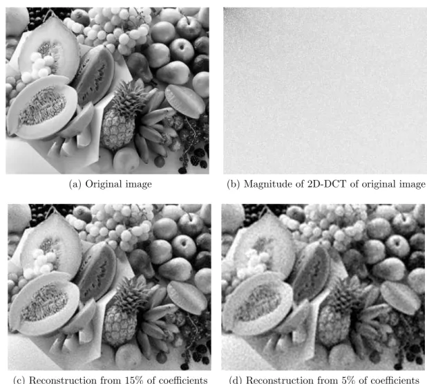
A frequently used transform to convert image intensities into the frequency domain is the two-dimensional discrete cosine transform (2D-DCT). One common use of the 2D-DCT is in the JPEG image compression standard. The 2D-DCT displays the energy compaction property more strongly than similar transforms such as the two-dimensional discrete Fourier transform (2D-DFT), and it can be calculated quickly and efficiently using fast Fourier transform (FFT) methods [5]. Figure 1-1 shows an image, its 2D-DCT coefficient magnitudes, and the images reconstructed by keeping only the top 15% and 5% of the coefficients by magnitude. The key features of the original image are preserved in the reconstructed images, and compression has been achieved in the sense that the reconstructed images are represented by fewer numbers.

(13)

(a) Original image (b) Magnitude of 2D-DCT of original image

(c) Reconstruction from 15% of coefficients (d) Reconstruction from 5% of coefficients

Figure 1-1: Example of 2D-DCT and the energy compaction property. 1-1(b) shows the 2D-DCT coefficients of 1-1(a), with larger magnitudes shown as darker. The reconstructed images 1-1(c) and 1-1(d) are generated by applying the inverse 2D-DCT on the top 15% and 5% of the coefficients from 1-1(b), respectively.

The transform coefficients must be quantized so that they can be represented by a finite sequence of bits. In quantization, each coefficient is mapped into one of a limited number of quantization levels based on which quantization interval the coefficient is in. This process introduces a further trade-off between quality and number of bits used. Larger quantization intervals introduce more error in the transform coefficients, but they require fewer bits to represent since there are fewer quantization levels and more coefficients are quantized to the zero level. Inversely, smaller quantization intervals allow the coefficients to be more accurately represented, but they require more bits

(14)

to specify and more coefficients are retained. By varying the size of the quantization intervals, the quality level of the reconstructed video and the required bitrate for transmitting the video can be adjusted. Quantized coefficients can then be coded as bit sequences through entropy coding methods, which use the quantized coefficients’ statistical properties to minimize the total number of coded bits [5].

In many applications of image and video compression, an image is split into blocks of pixels and transforms are then applied to individual blocks rather than the entire image. This approach has several advantages, including computational reduction and suitability for parallel processing. Block-by-block transform coding is also more adaptive to local characteristics, since blocks containing more details can be allocated more bits for coding than more uniform blocks. A disadvantage is that this can produce undesirable blocking artifacts in the resulting reconstructed image due to the blocks being coded independently of one another, creating artificial discontinuities at block boundaries. These negative blocking effects can be mitigated by dividing the original image into overlapping blocks [5].

In addition to spatial redundancies that can be exploited by using transforms, typical video sequences also show strong temporal redundancies. Most frames will differ only slightly from the frames immediately before and after, since the motion in typical videos is not fast. To take advantage of this characteristic, many video compression schemes use motion compensation (MC). In this method, the current frame to be encoded is first divided into blocks of pixels. For each block, a prediction is made by finding a closely-matching region from a previously encoded frame, which is referred to as the reference frame. To encode the block, the only data that is needed is the displacement between the location of the block in the current frame and the location of the prediction region from the reference frame. Motion compensation works well for regions undergoing translational motion, but it can be very inaccurate in high-detail regions. Therefore, the difference between the actual block and the predicted block is also coded so that a better representation of the original block can be reconstructed. This difference is known as the motion compensation (MC) residual. MC residuals can be treated as regular images and compressed using the

(15)

2D-DCT followed by quantization and entropy coding, which is the method used in widely-used video coding standards such as H.264/AVC [7].

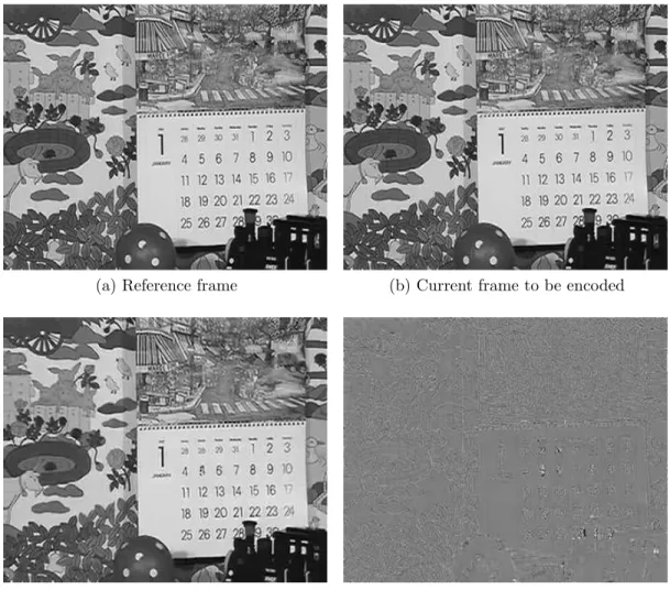
Figure 1-2 shows an example of motion compensation. Figures 1-2(a) and 1-2(b) are two frames in a video sequence, where Figure 1-2(a) is a frame that has been previously encoded and Figure 1-2(b) is the current frame to be encoded. Figure 1-2(c) shows the prediction for the current frame using Figure 1-2(a) as the reference frame, and Figure 1-2(d) is the MC residual. The MC residual is transformed us-ing the 2D-DCT, quantized, and then inverse transformed. Figure 1-2(e) shows the frame generated by adding the prediction from Figure 1-2(c) to the reconstructed MC residual.

As Figure 1-2(d) suggests, the MC residual is typically small in amplitude at most locations, meaning that motion compensation produces an accurate prediction at most pixels. Unlike regular images, most of the energy in the MC residual is located at boundaries and edges of objects and regions in the original frame, as well as highly-detailed regions. Since typical MC residuals exhibit even more spatial redundancy than regular images, MC residuals can usually be sufficiently represented by fewer transform coefficients than their corresponding original images, leading to more effective overall compression.

Spatial and temporal redundancies can be exploited in many other ways as well. The use of transforms and motion compensation are just two of the many aspects of video compression. The focus of this thesis is at the intersection of these two particular techniques: the transform step of MC residual coding.

(16)

(a) Reference frame (b) Current frame to be encoded

(c) MC prediction of current frame (d) Motion compensation residual

(e) Reconstructed current frame

Figure 1-2: Example of motion-compensated prediction. A motion-compensated pre-diction of the current frame is created using previously encoded blocks from the reference frame. The corresponding MC residual is shown, with mid-level gray repre-senting zero value. A reconstructed frame is generated from the blocks’ displacement vectors and the transformed and quantized MC residual.

(17)

1.2 Motivations for Thesis

The spatial characteristics of MC residuals differ greatly from those of regular images, indicating that transforms such as the 2D-DCT which are used for images may not provide the best performance when coding MC residuals. MC residuals often display locally anisotropic features in the sense that on a local scale, the high-amplitude values of MC residuals display some particular directionality. These features are fundamen-tally different from the anisotropic features found in regular images. MC residuals have high-amplitude intensities at object and region edges and low-amplitude inten-sities in smooth, stationary regions. On the other hand, regular images could have any intensity in a particular region, and object edges are characterized by differences in intensity rather than absolute intensity.

Since the characteristics of MC residuals and regular images differ, the transforms that perform well on regular images may not be the best transforms to use when coding MC residuals. Based on this observation, experiments have been performed by augmenting the H.264/AVC codec with a set of directional one-dimensional discrete cosine transforms (1D-DCTs) for use in MC residual coding [4]. The results have shown that using transforms that exploit the particular anisotropic properties of MC residuals can provide significant bitrate savings. However, extra calculations are required to optimize the selected transform for each block of every MC residual, which can potentially be costly and time-consuming in practice.

The goal of this thesis is to analyze the performance of 1D-DCTs for coding MC residuals to determine if their usage can be modified to reduce computation while still maintaining significant bitrate savings. We explore the performance of the H.264/AVC codec with access to different sets of transforms for MC residual coding. Experimental results show that most of the bitrate savings can be preserved by keeping only the horizontal and vertical 1D-DCTs in addition to the 2D-DCT. These results indicate that significant increases in compression efficiency can be made in comparison to the original codec without using a full set of directional 1D-DCTs, encouraging research in this direction for further improvements in video compression.

(18)

1.3 Overview of Thesis

Chapter 2 provides relevant further background and previous research performed in the area of video compression. Specific characteristics of MC prediction residuals are described, as well as techniques that have been developed to exploit them for improved compression. We review the results of using 1D-DCTs to code MC residuals.

Chapter 3 describes new experimental results and further analyses of the impact of using 1D-DCTs on MC residuals. We find that most of the benefit provided by using these transforms can be captured by using just the 1D-DCTs in the horizontal and vertical directions. We compare the performance of the H.264/AVC codec under three cases, each using a different set of transforms for encoding MC residuals.

Chapter 4 provides a summary of the results in the thesis, as well as directions for future related research.

(19)

Chapter 2 Previous Research

In this chapter, we review previous research related to the transform stage of cod-ing motion compensation (MC) prediction residuals. Section 2.1 describes results from analyses of the characteristics of MC residuals. In Section 2.2, we review a direction-adaptive transform technique based on 1D-DCTs that takes advantage of the anisotropic features found in MC residuals. Finally, Section 2.3 relates the find-ings and results from the earlier sections to the research in this thesis.

2.1 Characteristics of MC Residuals

The prediction residuals obtained by finding the differences between video frames and their motion compensation predictions have observably different characteristics from typical images. Because motion compensation is effective at predicting the local motions of blocks of pixels, most pixels in the MC prediction are very close in intensity to their corresponding pixels from the actual frame. Therefore, most pixels in the MC residual have intensities close to zero. This differs greatly from normal images, where the only regions of zero intensity are black regions. In addition, motion compensation often performs poorly in regions of high contrast, such as object edges and boundaries, arising in part from the fact that motion compensation assumes translational motion. Real motion in video sequences is often not strictly translational, so by assuming translational motion, the prediction is inaccurate near edges and boundaries. This is

(20)

reflected in the MC residual, which has high-magnitude intensities in these regions. Again, this contrasts with typical images, where edges are just the interfaces between regions of differing intensity.

The high-magnitude intensity pixels in MC residuals form local features aligned with object edges and boundaries. These local features are bordered by regions of low intensity on both sides, so they can be characterized as 1D features. On the other hand, on a local scale in normal images, edges are bordered by smooth regions of differing intensity on each side. Therefore, edge regions in normal images are characterized as 2D features. This fundamental difference motivates the usage of 1D transforms rather than 2D transforms for coding MC residuals.

Beyond these general empirical observations, studies have been done to statisti-cally quantify the differences between MC residuals and their corresponding original images. To apply statistical analysis to general video signals, models have been de-veloped in which images are represented as random processes. One basic model is the Markov-1 model, in which an image is modeled using a Markov process whose conditional distribution is dependent on only a single past value. Generalizing the auto-covariance function of the Markov-1 process to two dimensions produces the following auto-covariance function:

C(I, J) = ρ|I|1 ρ |J|

2 (2.1)

The parameters I and J represent the horizontal and vertical distances between the pixels for which the auto-covariance is given. The parameters ρ1 and ρ2 are cor-relation parameters in the horizontal and vertical dimensions, taking on values from 0 to 1. Assuming that images can be modeled by this auto-covariance equation, the correlation parameters can be estimated for sample video frames and MC residuals. Results indicate that in images, there is high spatial correlation between neighboring pixels, whereas the spatial correlation is significantly lower for MC residuals [6].

The auto-covariance model in Equation 2.1 produces estimates for correlation coefficients in the horizontal and vertical directions when I and J refer to horizontal

(21)

and vertical distances between pixels. It can be generalized to produce estimates for correlation coefficients in a general pair of orthogonal directions:

C(I, J, θ) = ρ|I cos θ+J sin θ|1 ρ

|−I sin θ+J cos θ|

2 (2.2)

The parameter θ represents the angle of rotation of the axes from the horizontal and vertical directions in relation to the model from Equation 2.1. It can easily be seen that when θ = 0◦_{, Equation 2.2 reduces to Equation 2.1. For each block, the} correlation parameters and angle of rotation can be estimated with a minimum mean squared error estimator [3]. By allowing the axes to rotate, this more general model can better characterize local regions of images and MC residuals, since different blocks may have different characteristics and therefore have different estimated values for θ, ρ1, and ρ2.

As described in [3], applying this generalized Markov-1 model to images and MC residuals produces several key results. Blocks in both images and MC residuals show strong correlation in one direction. However, in the perpendicular direction, the correlation is typically much weaker for MC residual blocks than for image blocks. This is consistent with the empirical observation that MC residuals exhibit more local 1D anisotropic features, while images exhibit more local 2D anisotropic features.

An additional result is that across all blocks for both MC residuals and images, the direction of strongest correlation is clustered around the horizontal and vertical directions (θ = 0◦_{, 90}◦_{, and 180}◦_{). Intuitively, this makes sense since typically, image} features are more often oriented in the horizontal and vertical directions than any other particular direction. For the MC residual blocks, this indicates that to take advantage of local 1D anisotropic redundancies, the most useful transforms are likely to be 1D transforms in the horizontal and vertical directions. This result is a primary motivation for the research presented in later chapters of this thesis.

(22)

2.2 Direction-Adaptive 1D-DCTs

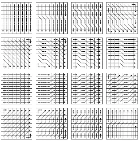
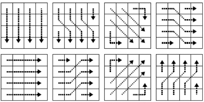
To exploit the characteristics of MC residuals described in the previous section, a set of directional 1D-DCTs was developed in [4] to code MC residual blocks using a modified H.264/AVC codec. These transforms apply to 8x8 and 4x4 pixel blocks, corresponding to the block sizes used in H.264/AVC. Figure 2-1 shows the set of sixteen directional 1D-DCTs that can be used on 8x8 blocks, and Figure 2-2 shows the set of eight directional 1D-DCTs that can be used on 4x4 blocks. To apply a particular directional 1D-DCT to a block, a regular 1D-DCT is performed on the sequence of pixels that each arrow passes through for every arrow shown in the block. Together, the directional 1D-DCTs in each set cover 180◦_.

In H.264/AVC, the block size for motion compensation is variable for different macroblocks and must be determined, along with the best transform to apply to each block. To select the block size for each macroblock and best transform for

(23)

Figure 2-2: Directional 1D-DCTs for coding 4x4 blocks in MC residuals.

each block, a Lagrangian-based rate-distortion optimization method that minimizes a mean squared error metric is used. Because the 2D-DCT may still work well for regions of the MC residual that do not have strong 1D anisotropic features, it is also included in the set of possible transforms to optimize over. After selecting the optimum block size and transform for a particular block, the transform is carried out and the transform coefficients are quantized. The quantized coefficients are then entropy coded using context-adaptive variable length coding (CAVLC).

The introduction of additional transforms means that side information must also be coded for each block to indicate which corresponding inverse transform should be applied to the block’s coefficients. To minimize the overall number of side information bits required, the transforms that are selected more frequently should be assigned codewords that are shorter than transforms that are selected less frequently. Based on the relative probabilities of selection for each different transform, [4] uses a 1-bit codeword for the 2D-DCT and 5-1-bit codewords for each 1D-DCT in the case of 8x8 blocks. For 4x4 blocks, the same 1-bit codeword is used to indicate the 2D-DCT, and 4-bit codewords are used for each 1D-DCT. Although this side information only contributes a small percentage of the total bits used to represent each block, a potential source of bit savings lies in shortening the side information codewords. This can be achieved by decreasing the number of transforms available to the codec to code MC residual blocks. If the only available 1D-DCTs are the transforms in the horizontal and vertical directions, then each block only has three transform options, and the 1D-DCTs can be represented by 2-bit codewords.

(24)

The experimental results from [4] show that adding the 1D-DCTs provides bitrate savings in all cases under the range of picture qualities used, which ranged from about 30dB to 40dB in PSNR. Moreover, the bitrate savings increase with picture quality. At higher picture qualities, a larger fraction of the total bitrate is used to code MC residual transform coefficients, so the bitrate savings provided by the 1D-DCTs is amplified compared to lower picture qualities. The compression was performed in three modes with different available block sizes, and the average bitrate savings over a range of picture qualities varied from 4.1% to 11.4%. The average percentage of the bitrate that was used to code side information ranged from 3.6% to 5.9%, which suggests that cutting the number of side information bits by a significant amount would have a small but noticeable impact on the overall bitrate.

2.3 Summary

The previous sections of this chapter have discussed research closely related to the transform stage of coding MC residuals. In Section 2.1, models for characterizing the statistical properties of images were presented. By applying these models to regular images and to MC residuals, it was found that MC residuals often display more local 1D anisotropic features than regular images, matching empirical evidence gathered from visual inspection. Based on this finding, it was hypothesized that direction-adaptive 1D transforms would be more effective in exploiting the directional 1D local correlations of MC residuals. Section 2.2 discussed an implementation of such a set of 1D transforms, the directional 1D-DCTs. The results obtained from using these additional transforms showed significant bitrate savings over using only the 2D-DCT to code MC residuals.

The results of Section 2.1 also indicate that the 1D anisotropic features in MC residuals are most frequently oriented in or close to the horizontal and vertical direc-tions. Based on this observation, the overall compression performance may not be significantly affected by removing the availability of all of the directional 1D-DCTs excluding the horizontal and vertical 1D-DCTs. In addition, as noted in Section 2.2,

(25)

reducing the number of available transforms would reduce the number of side infor-mation bits, which would help to compensate for the loss in performance of having fewer transform options to select from. In the next chapter, we apply these observa-tions and results in modifying the H.264/AVC codec to perform transform coding of MC residuals with different sets of available transforms.

(26)

(27)

Chapter 3 Experimental Results and Analysis

In this chapter, we present experimental results on the performance of using different sets of transforms for coding motion compensation residuals. Section 3.1 describes the implementation of the system used in obtaining the results. Section 3.2 provides the setup of the experiments, including the specific parameters used for the H.264/AVC codec. Sections 3.3 through 3.6 present data and comparisons for the compression efficiency of the three codec cases. Particular emphasis is given to comparisons be-tween the cases where all of the 1D-DCTs are available and where only the horizontal and vertical 1D-DCTs are available.

3.1 System Implementation

To analyze the performance of different sets of transforms in coding MC residuals, we further augment the modified H.264/AVC codec used in [4]. H.264/AVC is a modern video coding standard that is widely used in video applications, including in Blu-ray discs and streaming internet video programs. All of the aspects of video compression discussed in Chapter 1 are included in H.264/AVC. By building on an H.264/AVC codec, the results of this thesis can be easily compared to past and future research.

Details on 1D transform implementation, selection, and coding in the modified H.264/AVC codec can be found in [4]. The primary differences compared to the new system used in this thesis originate from the restriction of the set of available

(28)

transforms. When rate-distortion optimization is performed to select a transform for each block of an MC residual, the optimization is only done over the transforms that are indicated as available.

The implementation of the selected transform remains the same as in [4], but the side information indicating which transform was selected uses fewer bits when fewer transforms are available. The 2D-DCT is always assigned a 1-bit codeword, while each available 1D-DCT is assigned a codeword of length 1 + log2N, where N is the number of available 1D-DCTs for the block size being processed. This modified coding of side information is implemented at both the encoder and the decoder.

3.2 Experimental Setup

The modified H.264/AVC codec can be used in several different modes. For the results presented in this chapter, the codec was run using three different available transform block sizes: 4x4 only, 8x8 only, and both 4x4 and 8x8. In all cases, a transform is selected for each block, rather than forcing all four 4x4 blocks in each 8x8 block to use the same transform as in [4].

For each set of transform block sizes, we consider three cases for the set of trans-forms available for coding MC residuals. The first case (Case 1) uses only the 2D-DCT, which produces the basic unmodified codec. The second case (Case 2) uses the 2D-DCT and only the vertical and horizontal 1D-DCTs. The third case (Case 3) uses the 2D-DCT and all directional 1D-DCTs, which produces a codec used in [4]. Since there are three options for available transform block sizes and three options for available MC residual transforms, we have nine different codecs.

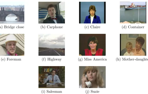
The test sequences on which we use these codecs are QCIF (177x144) resolution sequences at 30 frames per second (fps). Ten different sequences are used, whose first frames are shown in Figure 3-1. The first 180 frames of each sequence are encoded, or the entire sequence if it comprises fewer than 180 frames. The first frame is encoded as an I-frame, and the rest of the frames are encoded as P-frames.

(29)

(a) Bridge close (b) Carphone (c) Claire (d) Container

(e) Foreman (f) Highway (g) Miss America (h) Mother-daughter

(i) Salesman (j) Suzie

Figure 3-1: First frames of the QCIF resolution (176x144) test sequences used in the experiments.

from PSNR vs. bitrate rate-distortion data. The PSNR is given in dB, and it is calculated for the luminance component only, since the 1D-DCTs are only applied to the luminance component. The bitrate is given in kb/sec, and it represents the total bitrate for all encoded information. This includes transform coefficients for the luminance and chrominance components, displacement vectors, and side information. Since the chrominance components are typically undersampled in comparison to the luminance component, they contribute significantly less to the overall bitrate [4]. To obtain multiple PSNR vs. bitrate data points for each sequence, we vary the quantization parameter of the codec. Lower values of the quantization parameter produce higher quality reconstructions, usually giving a higher PSNR in exchange for a higher bitrate.

3.3 Rate-Distortion Plots

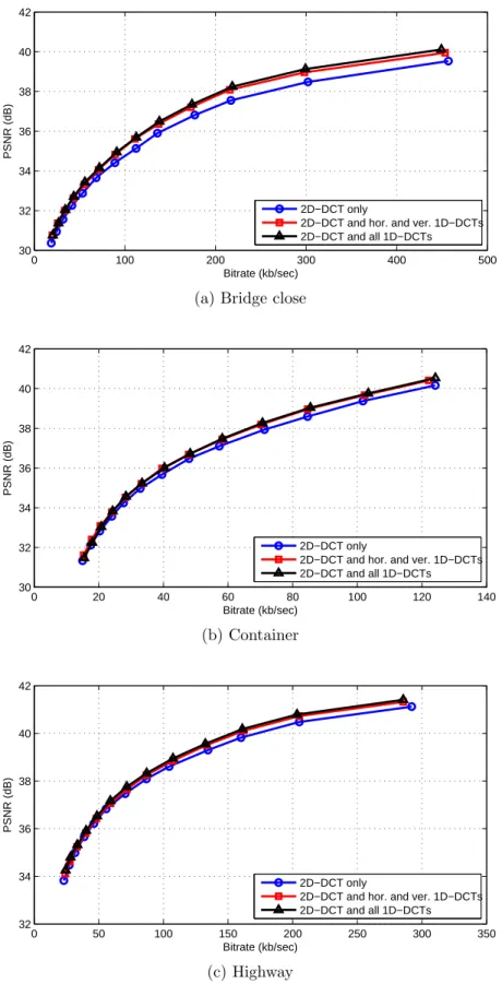
Figure 3-2 shows the rate-distortion plots for the Bridge close, Container, and

(30)

are shown, representing the three different sets of available transforms for MC residual coding.

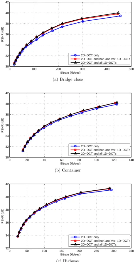
The data points are obtained by varying the H.264/AVC quantization parameter from 24 to 36 with a step size of 1, covering a PSNR range from about 30dB to 40dB. 30dB corresponds approximately to the low-quality video streaming used in many internet applications, while 40dB corresponds approximately to broadcast quality.

These plots show that at a given bitrate, the achieved PSNR increases as the set of available transforms expands. Equivalently, at a fixed PSNR, the required bitrate decreases as the set of available transforms expands. As seen in [4], the percentage bitrate savings over Case 1 increases at higher video qualities for Cases 2 and 3. A larger percentage of the bitrate is used to code transform coefficients at higher qualities, so the benefits of improved transform coefficient compression becomes more significant at higher qualities.

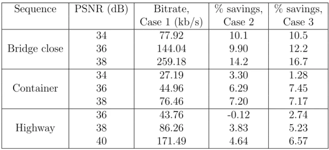
From Figure 3-2, based on how close the curves for Cases 2 and 3 are in comparison to Case 1, it is clear that using only the 2D-DCT and the horizontal and vertical 1D-DCTs can provide nearly all of the bitrate savings of using the 2D-DCT and all of the directional 1D-DCTs. Table 3.1 summarizes the bitrate savings as a percentage of the bitrate using only the 2D-DCT at fixed PSNR levels for the three sequences used in Figure 3-2. Again, Case 2 typically provides a substantial fraction of the bitrate savings that would be obtained by Case 3. In some cases, Case 2 even performs better than Case 3, such as for the Container sequence at PSNRs of 34 dB and 38 dB.

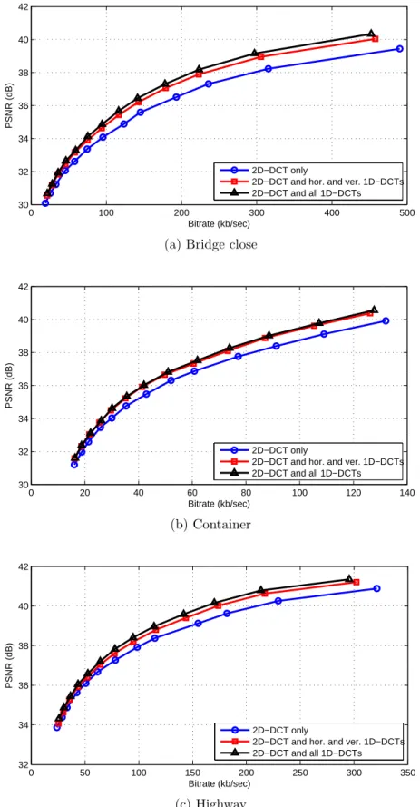
Similar results hold when different-sized blocks are available for the MC residual transforms. Figure 3-3 shows the corresponding rate-distortion plots using only 8x8 blocks, and Figure 3-4 shows the corresponding rate-distortion plots using both 4x4 and 8x8 blocks. As noted in [4], the addition of 1D transforms provides the greatest bitrate savings when only 8x8 blocks are used, while the bitrate savings is lowest when only 4x4 blocks are used. It can be seen from Figures 3-2, 3-3, and 3-4 that for all block sizes, using only the horizontal and vertical 1D-DCTs captures most of the bitrate savings provided by using 1D-DCTs. In Figure 3-3, the curves for cases 2 and 3 are not as close as in Figures 3-2 and 3-4, implying that the horizontal and

(31)

Sequence PSNR (dB) Bitrate, % savings, % savings,

Case 1 (kb/s) Case 2 Case 3

Bridge close 34 77.92 10.1 10.5 36 144.04 9.90 12.2 38 259.18 14.2 16.7 Container 34 27.19 3.30 1.28 36 44.96 6.29 7.45 38 76.46 7.20 7.17 Highway 36 43.76 -0.12 2.74 38 86.26 3.83 5.23 40 171.49 4.64 6.57

Table 3.1: Percent bitrate savings at fixed PSNR levels using 4x4 transform blocks only for three QCIF resolution test sequences.

vertical 1D-DCTs are less effective at capturing bitrate savings for 8x8 blocks than for 4x4 blocks. This can be viewed as a result of attempting to use the horizontal and vertical 1D-DCTs to replicate the performance of different numbers of transforms for the two different block sizes. Since 8x8 blocks have more total directional 1D-DCTs than 4x4 blocks, it is more difficult for just the horizontal and vertical 1D-DCTs to achieve the bitrate savings of all the 1D-DCTs for 8x8 blocks.

(32)

0 100 200 300 400 500 30 32 34 36 38 40 42 Bitrate (kb/sec) PSNR (dB) 2D−DCT only

2D−DCT and hor. and ver. 1D−DCTs 2D−DCT and all 1D−DCTs

(a) Bridge close

0 20 40 60 80 100 120 140 30 32 34 36 38 40 42 Bitrate (kb/sec) PSNR (dB) 2D−DCT only

2D−DCT and hor. and ver. 1D−DCTs 2D−DCT and all 1D−DCTs (b) Container 0 50 100 150 200 250 300 350 32 34 36 38 40 42 Bitrate (kb/sec) PSNR (dB) 2D−DCT only

(c) Highway

Figure 3-2: Rate-distortion plots using codecs with access to different sets of trans-forms and using 4x4 transform blocks only for three QCIF resolution test sequences.

(33)

(a) Bridge close

(c) Highway

Figure 3-3: Rate-distortion plots using codecs with access to different sets of trans-forms and using 8x8 transform blocks only for three QCIF resolution test sequences.

(34)

(a) Bridge close

(c) Highway

Figure 3-4: Rate-distortion plots using codecs with access to different sets of trans-forms and using both 4x4 and 8x8 transform blocks for three QCIF resolution test sequences.

(35)

3.4 Bjontegaard-Delta Bitrate Results

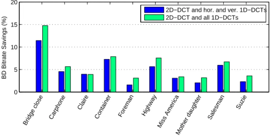
To compare the separation between the curves shown in Figure 3-2 over the different video sequences, the Bjontegaard-Delta (BD) bitrate metric is used [1]. This metric provides a measure of the average bitrate savings for an encoder with respect to another encoder over a range of quality levels. Figure 3-5 shows the BD bitrate metrics comparing Case 2 with Case 1 and comparing Case 3 with Case 1 for the ten QCIF test sequences. The three graphs correspond to the three different transform block size modes. The BD metrics are computed over a range of picture qualities corresponding to H.264/AVC quantization parameter values from 12 to 36.

We first consider the mode using 4x4 transform blocks only. For nine out of the ten video sequences, the average bitrate savings over all picture qualities is higher when all of the 1D-DCTs are available, in comparison to when only the horizontal and vertical 1D-DCTs are available. For the one sequence in which Case 2 gives higher average bitrate savings than Case 3 (Claire), the BD metrics are nearly identical. The average BD metric is 4.78% for Case 2 and 5.97% for Case 3.

In the two other block size modes, the average bitrate savings is higher when all of the 1D-DCTs are available for all of the video sequences. When only 8x8 blocks are used, the average BD metric is 12.20% for Case 2 and 16.55% for Case 2. When both 4x4 and 8x8 blocks are used, the average BD metric is 6.12% for Case 2 and 8.12% for Case 3. As seen from the rate-distortion plots in the previous section, the performance of Case 2 is closest to the performance of Case 3 when only 4x4 blocks are used, and furthest when only 8x8 blocks are used.

Based on Figure 3-5, Case 3 performs better on average than Case 2 in terms of bitrate savings. This verifies that the benefit of having better adaptive transforms typically outweighs the extra bits of side information needed for each block. However, the data also indicate that using only the horizontal and vertical 1D-DCTs captures a significant portion of the bitrate savings afforded by using all of the directional 1D-DCTs. For all test sequences in all block size modes, Case 2 provides more than 50% of the average bitrate savings that Case 3 provides in terms of the BD metric.

(36)

0 5 10 15 20

Bridge close Carphone Claire

Container Foreman Highway Miss America

Mother daughter Salesman

Suzie

BD Bitrate Savings (%)

(a) 4x4 transform blocks only

0 5 10 15 20 25 30 Bridge close Carphone Claire

Suzie

(b) 8x8 transform blocks only

0 5 10 15 20

Suzie

(c) 4x4 and 8x8 transform blocks

Figure 3-5: Bjontegaard-Delta bitrate savings for ten QCIF resolution test sequences as compared to the total bitrate when only the 2D-DCT is used.

(37)

3.5 Side Information Bitrates

To distinguish among the different possible transforms at the decoder in Cases 2 and 3, bits of side information are transmitted, contributing to the overall bitrate. Figure 3-6 shows the percentage of the total bitrate that comes from side information bits in Cases 2 and 3 using only 4x4 transform blocks, with each graph showing data from using a different value for the H.264/AVC quantization parameter.

As picture quality increases (or the quantization parameter decreases), the per-centage of the bitrate used for side information generally increases and then decreases, as seen in the progression in Figure 3-6. The initial increase is partially due to more and more blocks selecting a transform, rather than being quantized to all zeros. The H.264/AVC encoder checks to see if a block is quantized to all zeros, in which case no transform needs to be performed and thus no side information needs to be sent. In addition, the increasing frequency with which 1D-DCTs are selected as compared to the 2D-DCT contributes to the rise in percentage of total bitrate used by side informaion, since the 1D-DCTs use more bits of side information than the 2D-DCT. After a certain point, nearly all of the MC residual blocks that could benefit from using a transform are already being transformed, so the additional quality improve-ment comes primarily from finer quantization. More accurate quantization requires more bits to represent transform coefficients, increasing the total bitrate. At the same time, the amount of side information does not change significantly, since the number of blocks that are not zero-coefficient blocks is almost constant. Therefore, the side information takes up a decreasing fraction of the total bitrate.

Similar results hold in the two other block size modes. Figure 3-7 and Figure 3-8 show the same results as Figure 3-6 using respectively only 8x8 blocks and both 4x4 and 8x8 blocks. Comparing between the block size modes, the difference between the two cases is larger for 8x8 blocks than for 4x4 blocks. Case 3 always results in a higher percentage of the total bitrate being used to transmit side information. As we will examine further in Section 3.6, this is primarily due to codeword length, since the 1D-DCTs are selected at similar frequencies in the two cases.

(38)

0 5 10 15

Suzie

Bitrate Spent on Side Information (%)

(a) Quantization parameter = 36

0 5 10 15 Bridge close Carphone Claire

Suzie

2D−DCT and hor. and ver. 1D−DCTs 2D−DCT and all 1D−DCTs (b) Quantization parameter = 24 0 5 10 15

Suzie

(c) Quantization parameter = 12

Figure 3-6: Percentage of total bitrate that is used for side information for ten test sequences at three different quantization parameter levels, 4x4 transform blocks only.

(39)

0 2 4 6 8 10 12

Suzie

0 2 4 6 8 10 12 Bridge close Carphone Claire

Suzie

2D−DCT and hor. and ver. 1D−DCTs 2D−DCT and all 1D−DCTs (b) Quantization parameter = 24 0 2 4 6 8 10 12

Suzie

Figure 3-7: Percentage of total bitrate that is used for side information for ten test sequences at three different quantization parameter levels, 8x8 transform blocks only.

(40)

0 2 4 6 8 10 12 14 Bridge close Carphone Claire

Suzie

0 2 4 6 8 10 12 14 Bridge close Carphone Claire

Suzie

2D−DCT and hor. and ver. 1D−DCTs 2D−DCT and all 1D−DCTs (b) Quantization parameter = 24 0 2 4 6 8 10 12 14

Suzie

Figure 3-8: Percentage of total bitrate that is used for side information for ten test sequences at three different quantization parameter levels, 4x4 and 8x8 transform blocks.

(41)

Sequence Category Case 1 Case 2 Case 3 Bridge close 2D-DCT 1.20 0.51 0.48 Hor./vert. 1D-DCT 0.00 0.98 0.34 Other 1D-DCT 0.00 0.00 0.66 Zero-coefficient 98.80 98.52 98.52 Container 2D-DCT 0.92 0.50 0.55 Hor./vert. 1D-DCT 0.00 0.57 0.20 Other 1D-DCT 0.00 0.00 0.26 Zero-coefficient 99.08 98.93 98.99 Highway 2D-DCT 0.78 0.40 0.40 Hor./vert. 1D-DCT 0.00 0.53 0.21 Other 1D-DCT 0.00 0.00 0.34 Zero-coefficient 99.22 99.06 99.04

Table 3.2: Transform category frequencies for three video sequences using a quanti-zation parameter of 36, 4x4 transform blocks only.

3.6 Frequencies for Selection of Transforms

For each MC residual block that the H.264/AVC encoder processes, rate-distortion optimization is performed to select a transform. When a block consists entirely of transform coefficients that would be quantized to zero, there is no need to encode the block with any particular transform, so the encoder sends a codeword to indicate this information to the decoder. Therefore, each MC residual block is assigned one of the available transforms, or it is marked as a zero-coefficient block. Table 3.2 shows the percentages of MC residual blocks for the Bridge close, Container, and Highway QCIF video sequences that fall under the following transform categories: selected 2D-DCT, selected horizontal or vertical 1D-DCT, selected some other 1D-DCT, and zero-coefficient. Data is given for all three 4x4 block codec cases using a quantization parameter of 36. Table 3.3 shows the same information obtained using a quantization parameter of 24, and Table 3.4 shows the same information using a quantization parameter of 12.

For each sequence at a given quantization parameter level, the percentage of zero-coefficient blocks is similar among all three cases. This indicates that the addition of more transforms does not significantly affect blocks that were originally considered

(42)

Sequence Category Case 1 Case 2 Case 3 Bridge close 2D-DCT 19.46 6.75 5.00 Hor./vert. 1D-DCT 0.00 12.52 3.59 Other 1D-DCT 0.00 0.00 10.47 Zero-coefficient 80.54 80.73 80.93 Container 2D-DCT 12.51 5.27 5.21 Hor./vert. 1D-DCT 0.00 7.07 2.68 Other 1D-DCT 0.00 0.00 4.22 Zero-coefficient 87.49 87.66 87.89 Highway 2D-DCT 18.06 8.01 7.53 Hor./vert. 1D-DCT 0.00 10.00 3.28 Other 1D-DCT 0.00 0.00 7.03 Zero-coefficient 81.94 81.99 82.16

Sequence Category Case 1 Case 2 Case 3

Bridge close 2D-DCT 84.08 35.49 22.37 Hor./vert. 1D-DCT 0.00 48.98 18.38 Other 1D-DCT 0.00 0.00 43.78 Zero-coefficient 15.92 15.53 15.47 Container 2D-DCT 69.51 25.69 21.89 Hor./vert. 1D-DCT 0.00 40.86 16.22 Other 1D-DCT 0.00 0.00 27.68 Zero-coefficient 30.49 33.45 34.22 Highway 2D-DCT 87.77 40.36 30.16 Hor./vert. 1D-DCT 0.00 50.90 20.06 Other 1D-DCT 0.00 0.00 41.07 Zero-coefficient 12.23 8.74 8.70

(43)

to be zero-coefficient blocks. This is consistent with the fact that many MC resid-ual blocks are actresid-ually very close to being entirely zero, since motion compensation produces good predictions in most regions.

Another observation is that the percentages of blocks that select any 1D-DCT are fairly close for Cases 2 and 3. This indicates that a large fraction of the blocks that choose a non-horizontal, non-vertical 1D-DCT in Case 3 end up choosing either the horizontal or vertical 1D-DCT in Case 2. Therefore, while the horizontal and vertical 1D-DCTs are less efficient in terms of compression for these blocks, they still provide better performance than the 2D-DCT in most instances.

As the quantization parameter decreases, more of the blocks that choose a non-horizontal, non-vertical 1D-DCT in Case 3 switch to the 2D-DCT in Case 2. This is more clearly shown in Figure 3-9, which plots the percentage of MC residual blocks choosing any 1D-DCT versus the quantization parameter value. The percentages are very close at higher values of the quantization parameter, but begin to diverge roughly for quantization parameter values below 20. At lower values of the quantization parameter, fewer coefficients are quantized to zero. At sufficiently low values of the quantization parameter, the horizontal and vertical 1D-DCTs may not be able to produce any more zero coefficients than the 2D-DCT, and thus would not provide better compression than the 2D-DCT. The 2D-DCT is then favored since it requires fewer bits of side information.

(44)

15 20 25 30 35 0 10 20 30 40 50 60 70 80 90 100 Quantization Parameter

% of MC Residual Blocks Using Any 1D−DCT

(a) Bridge close

15 20 25 30 35 0 10 20 30 40 50 60 70 80 90 100 Quantization Parameter

2D−DCT and hor. and ver. 1D−DCTs 2D−DCT and all 1D−DCTs (b) Container 15 20 25 30 35 0 10 20 30 40 50 60 70 80 90 100 Quantization Parameter

(c) Highway

Figure 3-9: Percentage of MC residual blocks selecting any 1D-DCT for Cases 2 and 3 at quantization parameter levels from 12 to 36, 4x4 transform blocks only.

(45)

Chapter 4 Conclusions

4.1 Summary

In modern video coding standards, motion compensation residuals are frequently coded using 2D-DCT block transforms, which are the same transforms used to code normal images. However, there are fundamental differences between the character-istics of MC residuals and normal images. MC residuals qualitatively display more local 1D anisotropic features, whereas normal images display more 2D anisotropic features. This difference is corroborated quantitatively through the auto-covariance analyses presented in Section 2.1. One-dimensional transforms such as the directional 1D-DCTs typically provide better compression of MC residuals than two-dimensional transforms like the 2D-DCT, as discussed in Section 2.2.

When the full set of directional 1D-DCTs is made available to the H.264/AVC codec, the encoder must perform a rate-distortion optimization to select the best transform for each MC residual block. Including the original 2D-DCT, this means that for blocks of size 4x4, nine transforms must be carried out for each block in order to select the best transform. For blocks of size 8x8, seventeen transforms must be carried out for each block. Thus, the optimization process is computationally expensive, and could potentially be impractical in certain applications.

To address this issue, we considered reducing the number of transforms available for encoding MC residuals. The auto-covariance analyses indicated that the directions

(46)

of highest correlation in MC residuals tend to be close to horizontal and vertical, which motivated the usage of the horizontal and vertical 1D-DCTs only. By using only the 2D-DCT and the horizontal and vertical 1D-DCTs, the optimization process requires significantly fewer computations since only three transforms must be carried out for each block.

When the number of available transforms is reduced, we incur losses in overall compression efficiency, since the remaining transforms may not be suitable for adapt-ing to the local directional characteristics in some of the MC residual blocks. This is partially offset by a decrease in the amount of side information that needs to be transmitted to the decoder to signal which inverse transform to use. If the net losses are large, then the decrease in computation may not be worth the loss in compression efficiency.

To find the effects of using only the 2D-DCT and the horizontal and vertical 1D-DCTs, we modified a H.264/AVC codec so that it operated under three cases. Case 1 had only the 2D-DCT available for coding MC residuals. Case 2 added the horizontal and vertical 1D-DCTs, and Case 3 added the rest of the directional 1D-DCTs. The PSNR versus bitrate plots in Section 3.3 showed that Case 2 performs almost as well as Case 3 for the range of qualities found in typical video applications. For some video sequences at certain PSNR levels, Case 2 performs just as well or even better than Case 3. As picture quality increases, the gap in performance between Case 2 and Case 3 increases, since better-adaptive transforms are selected in Case 3.

Section 3.4 showed that averaging across all test sequences and quantization pa-rameter levels, Case 3 performs better than Case 2 in terms of the Bjontegaard-Delta bitrate metric. However, in the case of using only 4x4 blocks, the average BD metric is 4.78% for Case 2 and 5.97% for Case 3, so on average the horizontal and vertical 1D-DCTs capture most of the bitrate savings provided by using directional 1D-DCTs. The horizontal and vertical 1D-DCTs capture less of the bitrate savings when 8x8 blocks are used, but still more than 50% for all test sequences. As discussed in Sec-tion 3.5, Case 2 uses a smaller percentage of the total bitrate for side informaSec-tion than Case 3, which contributes to retaining bitrate savings even when most of the

(47)

1D-DCTs have been removed.

Finally, in Section 3.6, we examined the frequencies of selection for the different transforms. The data showed that at reasonable values for the quantization param-eter, most of the blocks that choose a directional 1D-DCT in Case 3 end up choos-ing either the horizontal or vertical 1D-DCT in Case 2, rather than the 2D-DCT. Therefore, in Case 2, the horizontal and vertical 1D-DCTs are still better suited for exploiting local 1D anisotropic features than the 2D-DCT, leading to bitrate savings that are close to the bitrate savings observed when all of the 1D-DCTs are available. Overall, the results presented in this thesis have demonstrated that significant bitrate savings can be achieved by adding the horizontal and vertical 1D-DCTs in coding MC residuals. Moreover, for quality levels found in most typical video ap-plications, these bitrate savings are close to the bitrate savings obtained by adding all of the directional 1D-DCTs. By using only the horizontal and vertical 1D-DCTs as opposed to all of the 1D-DCTs, the number of required computations is reduced while still maintaining comparable compression efficiency. We believe that these re-sults are promising, and future research can motivate further improvements in video compression.

4.2 Future Research

While the methods used in this thesis attempted to take advantage of the spatial and temporal correlations present in video sequences, there are additional correlations that can be exploited. For example, the selected transform for a particular MC residual block could be related to the transforms selected by its neighboring blocks. There could also be correlation between the displacement vector for a MC residual block and the type of transform that the block selects. From this information, a prediction can be made as to which transform would be selected, eliminating the need to transmit side information to the decoder for this block.

In reducing the number of available transforms, we chose to keep the horizontal and vertical 1D-DCTs because on average, the 1D features of MC residuals are more

(48)

often oriented in these directions. However, for a particular video sequence, these may not be the optimal pair of 1D-DCTs to have available for coding MC residuals. Our video compression scheme can be improved by adaptively choosing which two 1D-DCTs to keep based on the features of the video that is being processed. They can even be changed in the middle of processing the video based on information from the current and neighboring frames and MC residuals. The two available 1D-DCTs would be more adaptive to the characteristics of current MC residual, which could produce further bitrate savings.

Besides MC residuals, other types of prediction residuals also exist in video coding that could benefit from using 1D-DCTs. In particular, resolution enhancement (RE) residuals display similar 1D characteristics to MC residuals, so direction-adaptive 1D-DCTs should be able to provide better compression efficiency for RE residuals as well. Again, the horizontal and vertical 1D-DCTs alone may be able to maintain most of the bitrate savings obtained by using the directional 1D-DCTs.

The experiments in this thesis used a particular mode of operation for the H.264/AVC codec in which optimal transforms were selected for each block in a 16x16 macroblock. The codec can also be set so that all blocks in a 16x16 macroblock use the same trans-form. This mode could provide better performance since one transform selection is coded as side information for each macroblock, rather than for each block.

(49)

Bibliography

[1] G. Bjontegaard. Calculation of average psnr differences between rd-curves. VCEG

Contribution VCEG-M33, April 2001.

[2] C.-F. Chen and K.K. Pang. The optimal transform of motion-compensated frame difference images in a hybrid coder. Circuits and Systems II: Analog and Digital

Signal Processing, IEEE Transactions on, 40(6):393-397, Jun 1993.

[3] F. Kamisli and J. S. Lim. “Transforms for the motion compensation residual,”

IEEE ICASSP 2009, pp. 789-792, April 2009.

[4] F. Kamisli and J. S. Lim. “Video compression with 1-D directional transforms in H.264/AVC,” IEEE ICASSP 2010, pp. 738-741, March 2010.

[5] J. S. Lim, Two-Dimensional Signal and Image Processing. Prentice Hall, 1990. [6] A. Puri, H.-M.for motion-compensated coding. In Acoustics, Speech, and

Sig-nal Processing, IEEE InternatioSig-nal Conference on ICASSP 87, volume 12, pages 1063-1066, Apr 1987.

[7] I. E. G. Richardson, H.264 and MPEG-4 Video Compression: Video Coding for

Analysis of one-dimensional transforms in coding motion compensation prediction residuals for video applications

Analysis of One-Dimensional Transforms in

Coding Motion Compensation Prediction

Residuals for Video Applications

Harley Zhang

Author . . . .

Department of Electrical Engineering and Computer Science

May 20, 2011

Certified by . . . .

Jae S. Lim

Professor of Electrical Engineering

Thesis Supervisor

Accepted by . . . .

Dr. Christopher J. Terman

Chairman, Masters of Engineering Thesis Committee

Analysis of One-Dimensional Transforms in Coding Motion

Compensation Prediction Residuals for Video Applications

by

Harley Zhang

Abstract

Acknowledgments

Contents

List of Figures

List of Tables

Chapter 1

Introduction

1.1

Overview of Video Compression

1.2

Motivations for Thesis

1.3

Overview of Thesis

Chapter 2

Previous Research

2.1

Characteristics of MC Residuals

2.2

Direction-Adaptive 1D-DCTs

2.3

Summary

Chapter 3

Experimental Results and Analysis

3.1

System Implementation

3.2

Experimental Setup

3.3

Rate-Distortion Plots

3.4

Bjontegaard-Delta Bitrate Results

3.5

Side Information Bitrates

3.6

Frequencies for Selection of Transforms

Chapter 4

Conclusions

4.1

Summary

4.2

Future Research

Bibliography