BIST test pattern generator based on partitioning circuit inputs

BIST Test Pattern Generator Based on

Partitioning Circuit Inputs

by

Clara Sanchez

Submitted to the Department of Electrical Engineering and

Computer Science

in partial fulfillment of the requirements for the degrees of

Master of Engineering

and

Bachelor of Science in Computer Science and Engineering

at the

MASSACHUSETTS INSTITUTE OF TECHNOLOGY

May 1995

©

Massachusetts Institute of Technology 1995. All rights reserved.

Author

... ...

...

r

Department of Electrical Engineerng and Computer Science

r\

Certified

by ...

/ ...

Srinivas Devadas

Associate Professor

A

ccepted

by ... ... ...

. .

...

. .

Frederic

rgenthaler

Chairman, Departmental4n.a

,9-tee

on Graduate Students

OF TECHNOLOGY

AUG 1 01995 4,.

01

BIST Test Pattern Generator Based on Partitioning

Circuit Inputs

by

Clara Sanchez

Submitted to the Department of Electrical Engineering and Computer Science on May 23, 1995, in partial fulfillment of the

requirements for the degrees of Master of Engineering

and

Bachelor of Science in Computer Science and Engineering

Abstract

The test length required to achieve a high fault coverage for random pattern resis-tant circuits when using pseudorandom patterns is unacceptably large. In order to reduce this test length, the circuit inputs are partitioned based on a set of vectors generated by an ATPG tool for the faults that are hardest to detect. The partition is chosen by a simple heuristic of counting the number of ones and zeros in each bit position of the generated patterns and choosing to constrain the positions with the most homogeneity. By constraining these positions to their most common values, the likelihood of generating the desired patterns increases. The necessary constraints can be generated by any of a number of deterministic pattern generation schemes which adds flexibility over previous methods. This method can achieve orders of magnitude reductions in test length over a regular LFSR solution with only a small amount of additional hardware.

Thesis Supervisor: Srinivas Devadas Title: Associate Professor

Acknowledgments

I would like to thank Jayashree Saxena and the rest of the Texas Instruments Design Automation Division Test Project, my advisor, Srinivas Devadas, and my family and friends for all of their support.

Contents

1 Introduction

2 Review of BIST Test Pattern Generation Techniques

2.1 Pseudorandom Test Generation.

2.2 Deterministic Test Pattern Generation ...

3 Description of Test Pattern Generator

3.1 Evolution and Motivation.

3.2 Test Pattern Generator Scheme ... 3.3 Hardware Implementation.

4 Experimental Results

4.1 Benchmark Results . . . .

4.1.1 Test Length Results . . . 4.1.2 Hardware results.

4.2 Comparisons to Other Methods . 4.2.1 Test Length Comparisons 4.2.2 Hardware Comparisons . 5 Conclusion and Future Work

7 9 10 12 15 16 18 21 24 . . . .24 . . . .24 . . . .27 . . . .28 . . . 28 . . . .30 31

List of Figures

2-1 Linear Feedback Shift Register (LFSR) ... 10

3-1 Model of BIST test pattern generator using shift register ... 16

3-2 Partitioning Algorithm ... 19

List of Tables

3.1 Results of shift register approach on selected ISCAS85 and ISCAS89

benchmarks ... 17

4.1 Results of TPG Scheme on synthesis benchmarks ... 25 4.2 Results of varying thresholds of TPG Scheme on synthesis benchmarks 26 4.3 Results of varying the number of Step 1 LFSR patterns of TPG Scheme

on selected synthesis benchmarks ... . 26 4.4 Hardware required using implementation described in Chapter 3 . . . 28 4.5 Test length comparisons with other methods ... 29

Chapter 1

Introduction

VLSI designers and manufacturers must ensure that their products are defect free in order to remain competitive. Unfortunately as the size of designs grows it becomes increasingly difficult to test them using patterns applied from an external source due to high test application time and test storage requirements. One approach that has been used to alleviate this problem is Built-In Self Test (BIST) circuitry that gener-ates patterns internally to test the chip. Traditionally, pseudo-random test patterns generated by a Linear Feedback Shift Register (LFSR) have been applied. Asso-ciated with every LFSR is a feedback polynomial that determines the sequence of patterns that will be generated [1]. Unfortunately, as designs grow the number of pseudo-random test patterns that must be applied to achieve adequate fault coverage becomes prohibitive. Additionally, an increasing number of designs are being synthe-sized and it has been shown that many faults in these circuits are not easily detected by random patterns [9].

In order to reduce the number of patterns that must be applied to a circuit to achieve sufficient fault coverage, deterministic test pattern generators have been built into the circuit. Such generators require additional hardware and generate a specific set of patterns to test the circuit [1]. In this paper, we propose a BIST test pat-tern generator that partitions the circuit inputs into two sets. One set of inputs is constrained to a constant value, while the other set is fed with pseudorandom pat-terns of a predetermined length. This is repeated for different constraints on the first

set of inputs. Typically, the number of constraints to be applied is small. Finally, pseudrandom patterns are applied to both sets to detect easy faults. This approach reduces the test length for random pattern resistant circuits.

Chapter two reviews BIST test pattern generation techniques.

Chapter three describes motivation and previous work, the proposed partitioning algorithm, and a proposed hardware scheme to implement the generator.

Chapter four presents test length and hardware size results as well as comparisons with other methods.

Chapter 2

Review of BIST Test Pattern

Generation Techniques

There have been several approaches for designing test pattern generators for BIST. The goal of all of these solutions is to provide a set of test patterns that achieve high fault coverage in a short test length with small hardware overhead. One approach has been to use pseudo-random vectors to achieve the desired fault coverage. These methods typically have a low hardware overhead but unfortunately high fault coverage is only achieved with a very high test length. The work that has been done in this area will be discussed in Section 2.1. Another approach has been to design generators that produce a certain number of deterministic test vectors. These solutions concentrate on achieving high fault coverages with small test lengths but often at the expense of high hardware overheads. Section 2.2 describes these solutions. Pseudo-random vector solutions tend to produce long test lengths while deterministic solutions often result in much additional hardware. Therefore, many approaches have made a tradeoff between test length and hardware overhead by combining pseudo-random and deterministic techniques. One way to accomplish this is to identify the hard-to-detect faults in the circuits and generate deterministic vectors for these faults and then use pseudo-random patterns for the remaining faults. These methods are not always effective in achieving acceptable results for all circuits.

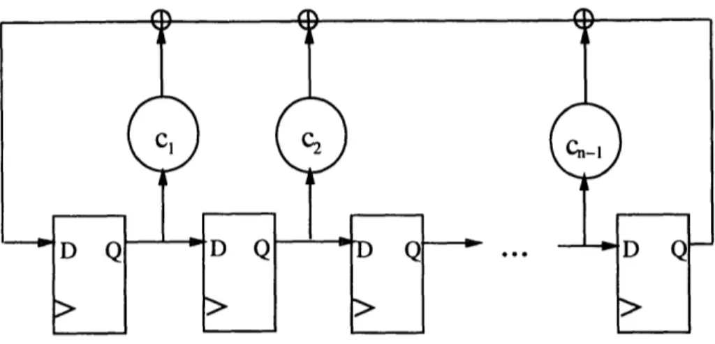
Figure 2-1: Linear Feedback Shift Register (LFSR)

2.1 Pseudorandom Test Generation

The most widely used source for pseudo-random patterns is the Linear Feedback Shift Register (LFSR). An n-bit LFSR consists of n memory elements and at most n 2-input XOR gates. A model of an LFSR is shown in Figure 2-1. Associated with every LFSR is a feedback polynomial that determines the sequence of patterns that will be generated [1]. For example, the LFSR in Figure 2-1 has the feedback polynomial 1 + cl * + 2 * 2 + .. + C - 1 * n - 1 + n where each of the ci's determines

whether there is a feedback connection from the output of the ith latch as shown in Figure 2-1. An n-bit LFSR will generate every n bit pattern except the all-zero pattern if its feedback polynomial is primitive [1]. LFSRs have been widely used to generate pseudo-random patterns because the hardware overhead associated is low. Unfortunately, as designs grow the number of pseudo-random test patterns that must be applied to achieve adequate fault coverage becomes prohibitive. Additionally, an increasing number of designs are being synthesized and it has been shown that many faults in these circuits are not easily detected by random patterns [9].

In order to reduce the test length required to achieve high fault coverages using an LFSR, a number of solutions have been proposed. One solution, proposed in [12], uses the theory of discrete logarithms to find out where the desired deterministic test vectors are in the sequence of pseudorandom patterns and uses this information to

embed the deterministic patterns in the smallest window of vectors in an LFSR se-quence of vectors by varying the feedback polynomial. Applying this method reduces the length of the test sequence by several orders of magnitude on most circuits but the test sequence is still very long for circuits with random pattern resistant faults. For example, in circuit in7 of the synthesis benchmarks, the test length was reduced from 56,544 to 9,274 by applying this method. In circuit xparc, however, the test length was reduced from more than 248 million patterns to about 133 million patterns, which is still unacceptably high[12]. Several solutions have been proposed that use a combi-nation of choosing the seed and feedback polynomial as well as using multiple seeds and multiple feedback polynomials to generate an LFSR sequence (or sequences) that achieves the desired fault coverage while reducing the test length [10, 8]. In both of these methods, extra hardware is used to make the LFSR configurable for multiple feedback polynomials as well as multiple seeds. Both require extra hardware and the reduction in test length was not analyzed. In [5], the authors reduce the size of the LFSR required by using the same LFSR cell for several compatible circuit inputs. This reduces the area overhead and reduces the pseudoexhaustive test length but the effect of this scheme on pseudorandom test length was not analyzed.

Another approach that has proven effective for some circuits has been to use weighted pseudo-random patterns [1]. In patterns produced by an ordinary LFSR, the probability of a particular bit being 1 is 0.5. If this probability were weighted to

w instead of .5, a modified LFSR results which no longer produces pseudo-random

patterns. The patterns produced by this LFSR can achieve the desired fault coverage in a much shorter test sequence if appropriate w's are chosen for each bit position. A weight set is defined as a vector of weights with one weight corresponding to each bit position. For example, for a 3-input AND gate, a complete test set consists of the vectors 011, 101, 110, 111. In this case, there is a 1 at each bit in 75% of the vectors. Therefore, an LFSR with weights of 0.75 at each bit produces 100% fault coverage with much fewer patterns than a normal LFSR. Much of the work in this area has focused on determining the weights to use at each bit and the number of different weight sets to use to achieve the desired fault coverage with a short test sequence

and acceptable additional hardware since additional weight sets require additional

controller hardware [4, 11].

A few solutions have limited the different possible weights to 0, 1, or 0.5, since producing each different weight requires additional hardware. This is equivalent to constraining certain bits to be 0 or 1 and letting the rest of the bits be generated by a regular LFSR. For each weight set, the bits that are constrained to a constant value

are those for which wi is 0 or 1. The method in [14] uses cube-contained random

patterns where certain bits are fixed to specific values (determined by the cube) for a group of patterns. In a method similar to [14], the authors in [15] compute the weight sets incrementally based on the faults not yet detected. Both these techniques require a more complex control hardware since the inputs that are assigned 0.5 weight vary with each weight set. The solution in [3] requires special Scan cells to fix certain bits as well as additional hardware to store the weight sets to be used. This solution does not limit the weights to 0, 0.5, and 1 but it does specifically choose the 0 and 1 weights before determining the other weights.

Although for many circuits pseudo-random techniques can provide adequate fault coverage without much additional hardware, there are many circuits which have ran-dom pattern resistant faults, and for these circuits, the test lengths become unac-ceptably large. For these circuits, test pattern generators that generate deterministic vectors must be used.

2.2 Deterministic Test Pattern Generation

In order to reduce the number of pseudo-random patterns that must be applied to a circuit to achieve sufficient fault coverage, deterministic test pattern generators have been designed that will generate a specific set of patterns to test the circuit. This requires additional hardware and there have been several proposed solutions that try to minimize the hardware overhead.

There have been two approaches for generating the desired patterns using a hard-ware generator. The first approach generates the patterns without any extraneous or

intermediate patterns. In the extreme case one could implement the desired function for each bit in the pattern but the hardware involved makes this approach impracti-cal. One can also use matrix manipulation to determine the feedback polynomial of the LFSR that generates the deterministic patterns as the first patterns in its pseu-dorandom sequence [19]. In this method, deterministic patterns are generated only for hard-to-detect faults and the easy faults are detected by the remaining patterns in the pseudorandom sequence. This method is appealing since no additional controller hardware is required and the method does not require extensive computation but un-fortunately, this method only generates as many deterministic patterns as the number of latches in the LFSR. For some circuits this still yields a very high test length. For example, using 500,000 pseudorandom patterns on the circuit xparc of the synthe-sis benchmarks still requires another 159 deterministic vectors while the circuit only has 39 inputs. If only 39 deterministic vectors could be used, the test length would increase greatly. In addition the hardware overhead increases since the polynomial will no longer be the one with the minimum number of feedback connections but will require an extra XOR gate for each additional feedback connection. The solution in [20] builds a Mixed-Output Autonomous Linear Finite State Machine (ALFSM) that generates deterministic vectors. This is an n-stage ALFSM with both complemented and uncomplemented register outputs. Each mixed-output ALFSM produces n n-bit vectors where at least n - 1 of these vectors are linearly independent. The hardware overhead for this is only slightly lower than for a regular ALFSM though which is usually too high. Another proposed solution has been to find a short sequence of pseudo-random vectors that includes the deterministic patterns and then implement hardware to skip over the extra vectors [17]. The method does not require seeds to be stored or to be scanned in, but the hardware overhead for this approach has been unacceptably high.

The other approach tries to generate the shortest sequence that contains the de-sired deterministic patterns. The authors in [2] generate a deterministic set of pat-terns by using an XOR grid to transform binary patpat-terns produced by a counter into the desired patterns. This method produces extraneous vectors in the sequence but

the authors then eliminate vectors in the deterministic test set which are no longer needed to achieve the same fault coverage. The XOR grid in this solution however often requires many XOR gates which is expensive though the method does have lower transistor counts than a ROM based approach. The approach used in [7] builds a finite state machine (FSM) that steps through vectors by changing one bit at a time and storing the position to be inverted for each transition in a ROM. The test sequence is built based on the deterministic patterns to be generated using an ad hoc heuristic. The ROM required in this method is smaller than in a ROM based approach but it does require some additional controller hardware and the test length is longer since extraneous vectors are generated. In [18], the authors use cellular automata (CA) with one and two rules to generate the deterministic patterns. The controller hardware depends on the number of deterministic patterns to be generated however and thus can get very large for circuits requiring many vectors. In [6], the author proposed the use of a shift register with a feedback function to generate the bit to be shifted into the first latch. The technique was only demonstrated for a small example, however. This work will be discussed in more detail in the next chapter since it was part of the motivation for the work described in this paper.

Each approach discussed in this chapter has a limitation which may or may not cause problems in relation to a particular circuit. The method proposed in the next chapter provides an alternative to the methods previously proposed.

Chapter 3

Description of Test Pattern

Generator

As was shown in the previous chapter, there have been many solutions aimed at achieving a desired fault coverage for combinational circuits in a short test length with small hardware overhead. The desired fault coverage we aimed for in solving this problem is 100%. The solution presented here makes a tradeoff between test length and additional hardware by partitioning the inputs of the circuit into two sets. Associated with one set is a set of input constraints. Test patterns are applied by two LFSRs. The first LFSR is loaded with the constrained values. For each constraint, the contents of this LFSR are frozen and the second is run normally for a fixed length. Once all the constrained patterns have been applied, both LFSRs run normally to generate pseudorandom patterns to complete the testing of easy faults. The solution described here is similar to the approaches in [14, 15] in that, for hard-to-detect faults, certain bits are constrained to 1 or 0 while others are generated pseudorandomly. The method differs significantly, however, in that the bit positions that will be constrained to 0 or 1 are the same for all the weight sets thus resulting in simpler control circuitry. This difference limits the flexibility of the bits we constrain but reduces the hardware requirement. Section 3.1 describes the motivation and previous work done based on [6]. Section 3.2 describes how to partition a circuit into inputs that will be constrained to 0 or 1 and inputs that will be fed by pseudorandom bits as well as determining

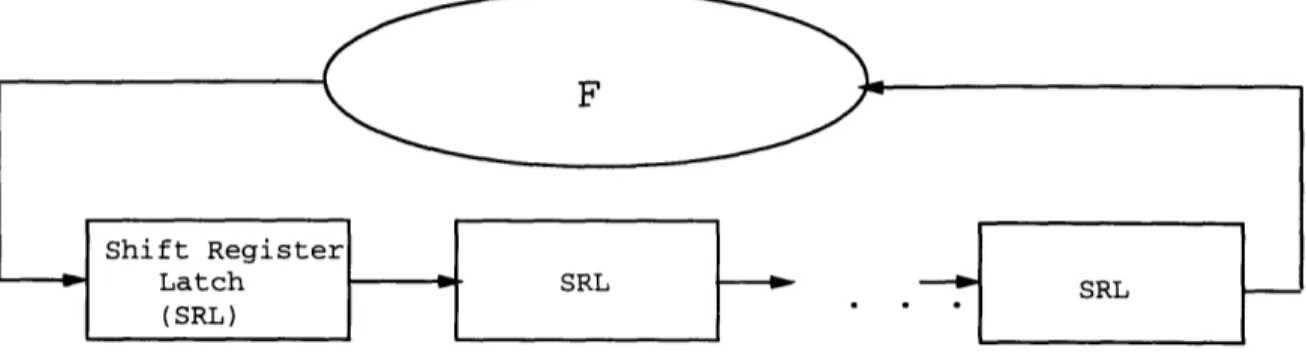
Figure 3-1: Model of BIST test pattern generator using shift register

the number of patterns to be used per constraint. Section 3.3 describes a possible hardware implementation of the generator.

3.1 Evolution and Motivation

This work began with the implementation of the approach in [6] and examining the results. The solution proposed in [6] to generate deterministic patterns in a BIST structure involves using a shift register with some feedback hardware. The basic model is shown in Figure 3-1. Suppose we want to generate the vectors v1, v2, ... , vn. A link vector is an intermediate vector that is required to get from one vector vi

to another vector vj in a shift register. For example to derive vector (100) from vector (010), the link vector (001) is required since at each step one bit can be shifted in from the left. The method proposed in [6] uses a nearest neighbor heuristic to build the sequence.

If we examine the problem of determining the shortest sequence of one bit shift vectors that includes the deterministic vectors, we can see that the problem can be represented as a weighted digraph where the nodes of the graph are the vectors to be generated and the weights on the edges are the number of shifts required to get from one vector to another. When formulated in this manner, the problem of finding the shortest sequence is equivalent to solving the Traveling Salesman Problem on the graph. Unfortunately, there is no bound on how far away the approximate solution presented in [6] is from the optimal solution.

#

c432 160 36 43 1202 74 252 c880 383 60 42 2304 117 423 c6288 2406 32 32 822 55 176 s349 161 24 22 397 29 95 s420.1 218 34 72 2022 112 365 s641 379 54 39 1881 105 377 s1238 508 32 150 3824 236 723 s1494 647 14 116 970 84 235

Table 3.1: Results of shift register approach on selected ISCAS85 and ISCAS89 bench-marks

Once the sequence is generated, the feedback function F that is needed can be derived as follows. For each vector v in the sequence, F(v) is equal to the first bit of the next vector in the sequence. Therefore, the hardware that implements this function will provide the correct bit to be shifted in for each vector. In the implementation, the hardware was synthesized using the Berkeley developed tools, espresso and SISII [16]. The results of applying this method using the nearest neighbor solution for finding the test sequence are shown in Table 3.1 for a few of the ISCAS85 and combinational portions of the ISCAS89 test benchmarks. The last column shows that the additional hardware required using gates with no more than 4 inputs using this scheme is between 10% and 175% of the circuit under test. The best results were achieved for those circuits with a high gate to input ratio.

It is clear that the nearest neighbor approach is not yielding an optimal solution as the length of test sequences in these examples is very close to the worst case length (# of test vectors x # of inputs). Undoubtedly, the results would improve if a more optimal solution were used to find the sequence since decreasing the length of the sequence causes a decrease in the amount of hardware needed. However, fundamentally this appr6ach does not take advantage of the way faults and especially hard to detect faults cluster in a circuit. Based on the deterministic patterns generated for the hard to detect faults in some random resistant circuits, we observed that the patterns generally have some kind of homogeneity where a particular bit pattern on

a subset of the bits appears in many patterns. Fundamentally, the shift register scheme does not work well for such patterns because as soon as one achieves that bit pattern the next shift disrupts it and many shifts are required to return to the bit pattern again. This behavior motivated us to look for a solution that partitions the problem and attempts to take advantage of the similarity in patterns to reduce the test sequence length and the hardware needed using a combination of deterministic and pseudo-random techniques.

3.2 Test Pattern Generator Scheme

The method proposed here partitions the circuit inputs into two sets. Each set of inputs is fed by a separate LFSR that can be controlled. The tests are applied in two separate phases. During the first phase, the first set of inputs are constrained to constant values. LFSR1, used to feed these inputs, is loaded with the appropriate constraints. The other set of inputs is fed by LFSR2 which functions normally. For each constraint, LFSR2 runs through vl pseudorandom patterns while LFSR1 is frozen at the constrained value. The second phase involves both LFSR1 and LFSR2 generating v2pseudorandom patterns. Thus if we use k constraints, the total number

of vectors that are applied is k x vl + v2. Figure 3.2 presents the algorithm that

determines the partition, constraints, and the lengths of vl and v₂.

The first step is to partition a circuit's inputs into constrained and unconstrained bits. Step 1 in Figure 3.2 generates deterministic patterns for random pattern resis-tant faults. In this case, this is done by fault simulating LFSR vectors and then run-ning Automatic Test Pattern Generation (ATPG) on the remairun-ning undetected faults. The number of LFSR vectors to fault simulate is chosen so as to keep the number of deterministic vectors generated not too large. A good heuristic is to run enough LFSR vectors to achieve 90% fault coverage (FC) although this does not always achieve the best results. We used a commercial test pattern generator FastscanTM [13] to per-form fault simulation and test generation. Test pattern generation took advantage of the pattern compression feature in FastscanT_{M [13].}

Step 1: Generating deterministic patterns for hard to detect faults. Fault

simu-late x pseudorandom vectors and get fault coverage FC. Perform ATPG for remaining

faults to obtain y deterministic patterns.

Step 2: Partitioning circuit inputs Use partition heuristic with threshold t, 0 < t < 1

to determine constraints.

Step 3: Fault simulation Fault simulate using constraints from Step 2.

* Let vl equal the number of LFSR2 vectors to be applied per constraint.

* Let v2 equal the number of unconstrained patterns to be applied in LFSR1 and

LFSR2.

* Let 3 equal the number of deterministic patterns needed to achieve 100% fault

coverage after the constrained and unconstrained patterns are applied.

* Fault simulate vl vectors per constraint plus v2 unconstrained vectors.

* Perform ATPG for remaining faults to get vs3 vectors.

* If V3= 0,

- Set vl equal to the maximum of the last effective pattern for each constraint. - Set v2 equal to the last effective unconstrained pattern.

* else,

- If one or more vectors in the set of v3deterministic vectors could be

gener-ated by the constrained patterns, increase vl.

- If no vectors in the set of 3 deterministic vectors can be generated by

the constrained patterns, increase v2. Do this up to 3 times; If still have

patterns in this second class, add a new constraint based on these patterns. - Repeat Step 3.

partition heuristic(threshold with 0 < threshold < 1)

* n equals the number of inputs to the circuit, k = number of constrained inputs

= threshold x n.

* Sort columns by decreasing maximum(number of zeros, number of ones).

* If there are more than k bits with maximum(number of zeros, number of ones) = n, then constrain all of these bit positions,

* Else choose k highest inputs from sorted list to be constrained.

* Constraints to be used are every unique bit pattern appearing in the constrained bit positions.

These vectors are then used to partition the circuit inputs into a set of bit posi-tions to be constrained and a set of constraints to use. The partition heuristic, also described in Figure 3.2 used in this scheme is a simple greedy heuristic using counts of zeros and ones in each bit position. Based on a threshold t between 0 and 1, the partition heuristic chooses t x n inputs to be constrained where n is the total number of circuit inputs. The inputs are chosen based on the homogeneity of the bits found in the vectors needed to detect the hard-to-detect faults in the circuit. The following example illustrates the partition heuristic.

Suppose the deterministic vectors determined by Step 1 are:

11111010 11011111 11111001 11111101 11110110 11010010 11111000 11110100

In this example, n = 8 and we set t = 0.5, thus the number of constrained bits, = 4. Counting the number of zeros and ones in each column:

1 0 8 8 1 2 0 8 8 2 3 2 6 6 4 4 0 8 8 3 5 3 5 5 5 6 4 4 4 7 7 4 4_ 4 48 8 5 3_ 5 6

Therefore, we choose to constrain the top 4 highest ranking bit positions which are bit positions 1, 2, 3 and 4. The constraints we use would be every bit pattern appearing in these bit positions. In this case, we would constrain bit positions 1-4 to

k

the constraints 1111 and 1101.

Once we have a partition with a set of constraints to be used, the number of pat-terns per constraint generated by LFSR2 and the number of unconstrained patpat-terns generated by both LFSRs must be found so that 100% fault coverage is achieved. This is essentially done by trying certain numbers of constrained and unconstrained vectors, fault simulating them, running ATPG for the remaining faults, and modify-ing the numbers of patterns accordmodify-ing to the fault simulation and ATPG results. This often requires several iterations to achieve 100% fault coverage. In some cases, the list of constraints is supplemented with additional constraints based on the patterns for those faults not yet covered. This is described in Step 3 of Figure 3.2.

This process partitions the inputs of the circuit so that the problem of testing the circuit can be divided into a deterministic test generation portion and a pseudorandom part which reduces the test length required to achieve high fault coverage. The next section contains a possible hardware implementation that shows how these constraints are used to generate patterns.

3.3 Hardware Implementation

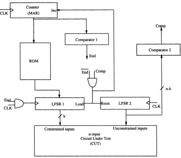
The structure used for the test pattern generator described here involves using two smaller LFSRs in place of one larger LFSR as shown in Figure 3-3. One LFSR (the one labeled LFSR1 in Figure 3-3 would be constrained to the constraints determined by the partitioning algorithm described in Section 3.2 and which are stored in the ROM. LFSR1, which is k bits wide, must be made up of multiplexed latches that can take data either from the ROM or from the previous stage of the LFSR. LFSR2 is n - k bits wide and these latches must be resettable. This allows the LFSR to be reset for each constraint after which vl random patterns are applied. Instead of using a counter that requires log2vll memory elements to count vl patterns, a

comparator can now be used to detect the final state after vl patterns are applied. The comparator requires at most 2(n - k) two input AND gates or inverters. The comparator (referred to as Comparator 2) is used to detect when vl patterns have

Figure 3-3: Hardware implementation of test pattern generator

been applied and the Memory Address Register (MAR) must be incremented in order to load the next constraint into LFSR1. This is also when LFSR2 resets. When vl patterns have been applied for all constraints, then Comparator 1 enables the End signal which enables LFSR1 to run in pseudorandom mode. Both LFSRs now run in pseudorandom mode for v2 more patterns.

One of the advantages of the proposed partitioning scheme that restricts itself to the same set of inputs is that the constraints needed for the first LFSR can be gener-ated by any of the many schemes that have been developed for deterministic pattern generation. The patterns that must be generated now however are much fewer and

not as wide. The method can be chosen based on the specific constraints that must be generated. Hardware size results as well as comparisons of this implementation with comparable methods is done in the next chapter.

Chapter 4

Experimental Results

The method described in the previous chapter makes a tradeoff between test length and hardware overhead. The solution performs best for random pattern resistant circuits where it can reduce the test length significantly. The results provided in this chapter demonstrate this. The next section provides the results of applying this method on a set of synthesized combinational logic Berkeley benchmarks. Section 4.2 compares this method with results obtained using comparable methods.

4.1 Benchmark Results

4.1.1 Test Length Results

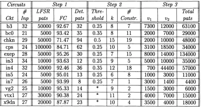
The results are presented for a set of synthesized combinational logic Berkeley bench-marks. These circuits are characterized by having random pattern resistant faults which yield very high pseudorandom test lengths. The results with the shortest test length obtained using this method are shown in Table 4.1. The column entitled To-tal pats in Table 4.1 shows the number of patterns required to achieve 100% fault coverage using this method.

In Table 4.1, the first 2 columns provide basic circuit information. The next 3 columns provide the data collected from Step 1 of the partitioning algorithm. Column 3 shows the number of pseudorandom patterns used in Step 1. Column 4 shows the

Circuits Step 1 Step 2 Step 3

# LFSR Det. Thre- # Total

Ckt Inp pats FC pats shold

1k

b3 32 50000 92.67 32 0.25 8 7 7300 12000 63100 bcO 21 5000 93.42 35 0.35 8 11 2000 7000 29000 chkn 29 50000 71.47 94 0.5 15 19 2000 10000 48000 cps 24 100000 84.71 62 0.25 10 5 3100 18500 34000 exep 28 50000 95.26 30 0.25 7 15 8000 14000 134000 in3 34 10000 93.63 12 0.25 9 5 5000 10000 35000 in4 32 50000 92.46 36 0.35 12 18 700 44400 57000 in5 24 5000 95.01 13 0.25 6 8 1000 3000 11000 in7 26 5000 93.99 8 0.25 7 1 3000 1400 4400 vg2 25 10000 95.33 14 * 9 2 1500 3000 6000 vtxl 27 30000 90.38 24 * 11 2 4000 7000 15000 x9dn 27 20000 87.87 23 10 4 3500 4000 18000

Table 4.1: Results of TPG Scheme on synthesis benchmarks

fault coverage achieved by the pseudorandom patterns. The number of deterministic patterns needed to raise the fault coverage to 100% is shown in Column 5. The next 3 columns provide the threshold and partitioning and constraints results from Step 2. Column 6 shows the threshold used by the partition heuristic. Column 7 shows the number of bits that were constrained. Column 8 shows the number of constraints that were obtained by the partition heuristic. The next 3 columns give the number of constrained, unconstrained, and total patterns used to achieve 100% fault coverage. Column 9 shows the number of patterns to be applied per constraint. Column 10 shows the number of unconstrained patterns to be applied. The last column shows total number of patterns to be applied. The partition heuristic used in this scheme performs well on many random pattern resistant circuits but there are circuits for which this simple heuristic fails to generate a useful partition such as circuits vg2,

vtxl, and x9dn in Table 4.1 which were partitioned by hand and thus no threshold

was used to achieve the results in the table. In these circuits, there were almost equal numbers of zeros and ones in each column although the bits were correlated so that there were actually only a few different bit patterns. For example, the vectors

(11111010,11110010,00001111,00000001) have equal numbers of zeros and ones in the first 4 bit positions even though there are only two patterns in these 4 positions,

Circuits Step Step 2 Step 3

I] l

LFSR

Det. Thre-

#

Total

Ckt Inputs pats FC pats shold

k

bc 21 5000 93.42 35 .25 6 6 4000 12000 36000 bcO 21 5000 93.42 35 .35 8 11 2000 7000 29000 bcO 21 5000 93.42 35 .5 11 21 L 500 15500 26000 in3 34 10000 93.63 12 .25 9 5 5000 10000 35000 in3 34 10000 93.63 12 | .35 12 6 2000 34000 46000 in3 34 10000 93.63 12 .5 17 13 400 50000 55200 in7 26 5000 93.99 8 [ .25 7 1 3000 1400 4400 in7 26 5000 93.99 8 [[ .35 10 4 500 4100 6100 in7 26 5000 93.99 8 || .5 13 5

If

Circuits Step 1 Step 2 Step 3

1#

n LFSR Det. Thre- # Total

Ckt Inp pats FC pats shold k Constr. vl v2 pats

chkn 29 50000 71.47 94 .35 11 6 15000 4000 94000 chkn 29 100000 75.05 90 .35 11 5 15000 4000 79000 chkn 29 500000 84.67 68 .35 11 6 15000 9000 99000 chkn 29 111500000 90.62 45 .35 12 6 10000 18000 78000 cps 24 50000 80.91 73 .35 9 3 10000 23000 53000 cps 24 500000 95.09 20 .35 11 6 2500 22000 37000 in4 32 10000 85.10 72 .35 12 35 2000 12000 82000 in4 32 50000 92.46 36 .35 12 18 700 44400 57000

Table 4.3: Results of varying the number of on selected synthesis benchmarks

Step 1 LFSR patterns of TPG Scheme

0000 and 1111. The heuristic in these cases fails to generate a useful partition. In order to obtain the results in Table 4.1, the algorithm was run varying several parameters. Table 4.2 shows results of experiments where the threshold in Step 2 is varied for a few of the benchmarks. Each circuit was run for threshold values of 0.25,

0.35, and 0.5.

It is important to note that no one threshold value did better for all circuits than the others. For example, for circuit bcO, increasing the threshold reduced the total number of patterns required while for circuit in3, the number of patterns required increased.

Another parameter that can affect the results is the number of LFSR patterns simulated in Step 1 which affects the number of deterministic patterns used in the partitioning algorithm. Results of varying the number of LFSR patterns in Step 1 for circuits chkn, cps, and in4 are shown in Table 4.3. The tendency is for test length to decrease when the number of LFSR patterns in Step 1 increases but this does not always occur as can be seen in Table 4.3 in circuit chkn where increasing the LFSR patterns in Step 1 from 100, 000 to 500, 000 increased the overall test length of the TPG scheme. Increasing the LFSR pattern count in Step 1 has the effect of decreasing the number of deterministic patterns on which the partition heuristic is run. This presumably has the effect of having the partition heuristic be based on fewer, harder to detect faults. Sometimes this generates a partition and constraints that target the hard to detect faults better but in other cases it may not target some hard to detect faults which then drives the test length up.

The hardware required for this test pattern generation scheme is presented in

Section 4.1.2 below.

4.1.2 Hardware results

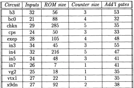
The hardware required to achieve the test lengths given in Table 4.1 is shown in Table 4.4. The first two columns in the table give circuit information. The column labeled ROM size gives the number of bits required to store the constraints in the ROM. This is computed by multiplying the number of bits constrained by the number of constraints. The next column, labeled Counter size, gives the width of the MAR for the ROM. The last column gives the number of 2-input gates required for the two comparators and the two additional AND gates shown in Figure 3-3.

The results presented in this section are compared with comparable methods in

Circuit Inputs ROM size Counter size Add'l gates b3 32 56 3 53 bcO 21 88 4 32 chkn 29 285 5 35 cps 24 50 3 33 exep 28 105 4 48 in3 34 45 3 55 in4 32 216 5 47 in5 24 48 3 41 in7 26 7 1 41 vg2 25 18 1 35 vtxl 27 22 1 35 x9dn 27 92 2 38

Table 4.4: Hardware required using implementation described in Chapter 3

4.2 Comparisons to Other Methods

The method described makes a tradeoff between hardware and test length and there-fore its test length results and hardware requirements must be compared to other methods to ascertain its advantages. Section 4.2.1 compares test length results with other methods. Section 4.2.2 compares the hardware size with that of previous meth-ods.

4.2.1

Test Length Comparisons

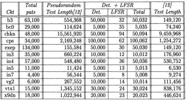
Table 4.5 compares the test length results achieved with this method (Column 2) to test lengths using pseudorandom patterns (Column 3), a few deterministic patterns plus pseudorandom patterns (Columns 4-6), and the method in [12] (Column 7).

This method achieves a significant reduction in test length over applying just pseudorandom patterns as can be seen when comparing columns 2 and 3 of Table 4.5. The method has a shorter test length in some circuits when compared to using both deterministic and LFSR patterns. It also achieves a reduction when compared with the method in [12]. As can be seen from Table 4.5, the circuits for which the proposed method achieved the best test length decreases were those which were most difficult to test with pseudorandom patterns such as chkn and cps. For chkn, the method in

Total Pseudorandom Det. + LFSR [12]

Ckt pats Test Length[12] Det.

1

b3 63,100 554,368 50,000 32 50,032 149,120 bc0 29,000 114,624 5,000 35 5,035 74,240 chkn 48,000 15,561,920 50,000 94 50,094 9,459,968 cps 34,000 2,169,248 100,000 62 100,062 1,254,272 exep 134,000 155,584 50,000 30 50,030 149,120 in3 35,000 660,224 10,000 12 10,012 176,960 in4 57,000 548,480 50,000 36 50,036 530,752 in5 11,000 11,424 5,000 13 5,013 6,530 in7 4,400 56,544 5,000 8 5,008 9,274 vg2 6,000 267,552 10,000 14 10,014 111,456 vtxl 15,000 1,345,152 30,000 24 30,024 838,176 x9dn 18,000 1,022,944 20,000 23 20,023 446,624

Table 4.5: Test length comparisons with other methods

[12] yields a test length of more than 9 million patterns while the proposed method yields a test length of only 48,000 patterns. Likewise for cps, the test length in [12] is more than 1 million patterns while the proposed method test length is 34,000.

For this class of circuits, the method in [19] does not yield a short test length since only n deterministic patterns can be applied where n, the number of circuit inputs, equals 29 for chkn and 24 for cps. In [5], the authors do not provide test lengths for these circuits but they do provide the size of the reduced LFSR that is needed to test the circuits. Using this information, we can examine the worst case test length using the method in [5]. For example, for chkn a 20-bit LFSR is needed. The worst case test length therefore is 220 > 1, 000, 000. Therefore, the proposed method achieves a solution with reasonable test length for these cases. Short test lengths for these benchmarks have also been reported in [14]. However, it is difficult to compare with results in [14] as the authors use randomly generated patterns instead of LFSR generated patterns. More importantly, they do not specify whether they have used a varying or fixed length random pattern set for each cube or weight set. Using a varying length set reduces test length but will cause an enormous increase in control complexity and hence hardware. It can be expected that the method in [15] will produce short test lengths for these benchmarks. However, the complexity

of controlling test application is higher in [15].

4.2.2 Hardware Comparisons

The hardware required by the implementation described can be compared with some of the other methods. For example, to compare this method with using a ROM to store a few deterministic patterns and then applying pseudorandom patterns we can use the second and fourth columns of Table 4.1 to determine one possible ROM size and test length for these circuits. The method proposed here achieves much lower ROM size for most circuits and especially for the most random pattern resistant ones. The method in [14] requires a MUX for every input and two bits of storage per input. In addition, although not described in the paper, the method would require a counter to count the pseudorandom patterns. In our method, the counter is replaced by a comparator and MUX capabilities are required only for a subset of inputs. The width of the ROM is smaller as well. In the method proposed in [15], again, MUXing may be required for many inputs. Further, the hardware described in [15] uses a counter to determine which constraint (or expanded test as it is called in [15]) is being used. Logic that is based on the counter values assigns inputs either a constant 0 or 1 or a pseudorandom value. However, the hardware required to step the counter is not mentioned in the paper. Both of the methods in [12] and [5] do not require additional hardware over that of an LFSR but for many circuits with hard to detect faults, these methods still do not achieve reasonable test lengths while this method does.

One of the advantages of the proposed partitioning scheme that restricts itself to the same set of inputs is that the constraints needed for the first LFSR can be generated by any of the many schemes that have been developed for deterministic pattern generation. The patterns that must be generated now however are much fewer and not as wide. The method can be chosen based on the specific constraints that must be generated.

Chapter 5

Conclusion and Future Work

The method described is an approach that makes a tradeoff between test length and hardware overhead. It provides an alternative to the set of possible test pattern generation methods and for some circuits yields better results than existing methods. The method produces the best results on those circuits with random pattern resistant faults for which other methods fail to produce solutions with practical test lengths with a reasonable hardware overhead. The method is also flexible enough that it can be adapted to achieve better results on individual circuits by choosing a deterministic pattern generation scheme based on the constraints to be generated. Another way to improve the results is to try several simple heuristics like the one proposed to find the one that yields the best results. By varying the number of constrained pins this solution covers the entire spectrum from pseudorandom to deterministic so that a designer can choose the place on the spectrum that is best suited to the circuit to be tested.

Future work on this method would develop the partition heuristic to improve the partition and therefore achieve better results. Several heuristics may need to be de-veloped that perform well on certain classes of circuits. Another possible development of this work would be to use an ATPG tool that generated vectors with don't cares. The partition heuristic would then need to be modified to take this into account but the partitioning would more accurately reflect the bit positions which influence the detection of the hard to detect faults. This method provides a basis on which to build

more sophisticated techniques for partitioning a circuit and combining deterministic and pseudorandom approaches to produce efficient test pattern generators.

Bibliography

[1] Miron Abramovici, Melvin A. Breuer, and Arthur D. Friedman. Digital Systems

Testing and Testable Design. Computer Science Press. New York, 1990.

[2] Sheldon B. Akers and Winston Jansz. Test set embedding in a built-in self-test environment. Proceedings IEEE International Test Conference, pp. 257-263,

1989.

[3] Mohammed F. Alshaibi and Charles R. Kime. Fixed-biased pseudorandom built-in self-test for random pattern resistant circuit. Proceedbuilt-ings IEEE International

Test Conference, pp. 929-938, 1994.

[4] Michael Bershteyn. Calculation of multiple sets of weights for weighted random testing. Proceedings IEEE International Test Conference, pp. 1031-1040, 1993. [5] C.-A. Chen and S. K. Gupta. A practical BIST TPG design methodology.

Tech-nical Report Number No. CENG-94-34, University of Southern California, 1994.

[6] W. Daehn and J. Mucha. Hardware test pattern generation for built-in testing.

Proceedings IEEE International Test Conference, pp. 110-113, 1981.

[7] Ramaswami Dandapani, Janak H. Patel, and Jacob A. Abraham. Design of test pattern generators for built-in test. Proceedings IEEE International Test

Conference, pp. 315-319, 1984.

[8] C. Dufaza and G. Cambon. LFSR based deterministic and pseudo-random test pattern generator structures. Proceedings 2nd European Test Conference, pp.

[9] S. K. Gupta and C. H. Chiang. Random Pattern Testable Logic Synthesis.

Technical Report CENG 94-08, University of Southern California, 1994.

[10] Sybille Hellebrand, Steffen Tarnick, and Janusz Rajski. Generation of vector patterns through reseeding of multiple polynomial linear feedback shift registers.

Proceedings IEEE International Test Conference, pp. 120-129, 1992.

[11] Rohit Kapur, Srinivas Patil, Thomas J. Snethen, and T. W. Williams. Design of an efficient weighted random pattern generation system. Proceedings IEEE

International Test Conference, pp. 491-500, 1994.

[12] Mody Lempel, Sandeep K. Gupta, and Melvin A. Breuer. Test embedding with discrete logarithms. Proceedings IEEE VLSI Test Symposium, pp. 74-80, 1994. [13] Mentor Graphics Inc. Fastscan User's Manual.

[14] Stephen Pateras and Janusz Rajski. Cube-contained random patterns and their application to the complete testing of synthesized multi-level circuits. Proceedings

IEEE International Test Conference, pp. 473-482, 1991.

[15] Irith Pomeranz and Sudhakar M. Reddy. 3-weight pseudo-random test generation based on a deterministic test set for combinational and sequential circuits. IEEE

Transactions on CAD, pp. 1050-1058, 1993.

[16] Ellen M. Sentovich et al. SIS: A system for sequential circuit synthesis.

Memo-randum No. UCB/ERL M92/41, University of California, Berkeley, Electronics

Research Laboratory, 1992.

[17] Shambhu J. Upadhyaya and Liang-Chi Chen. On-chip test generation for com-binational circuits by LFSR modification. Proceedings IEEE International

Con-ference on CAD, pp. 84-87, 1993.

[18] Jon van Sas, Francky Catthoor, and Hugo De Man. Optimized BIST strategies for programmable data paths based on cellular automata. Proceedings IEEE International Test Conference, pp. 110-119, 1992.

[19] Beena Vasudevan, Don E. Ross, Murali Gala, and Karan L. Watson. LFSR based deterministic hardware for at-speed BIST. Proceedings IEEE VLSI Test

Symposium, pp. 201-207, 1993.

[20] L.F.C. Lew Yan Voon, C. Dufaza, and C. Landrault. BIST linear generator based on complemented outputs. Proceedings IEEE VLSI Test Symposium, pp.