H-infinity control of an irrigation canal pool with a mixed control politics

HAL Id: hal-00450870

https://hal.archives-ouvertes.fr/hal-00450870

Submitted on 27 Jan 2010

HAL is a multi-disciplinary open access

archive for the deposit and dissemination of

sci-entific research documents, whether they are

pub-lished or not. The documents may come from

teaching and research institutions in France or

abroad, or from public or private research centers.

L’archive ouverte pluridisciplinaire HAL, est

destinée au dépôt et à la diffusion de documents

scientifiques de niveau recherche, publiés ou non,

émanant des établissements d’enseignement et de

recherche français ou étrangers, des laboratoires

publics ou privés.

mixed control politics

X. Litrico, V. Fromion

To cite this version:

X. Litrico, V. Fromion. H-infinity control of an irrigation canal pool with a mixed control politics.

IEEE Transactions on Control Systems Technology, Institute of Electrical and Electronics Engineers,

2006, 14 (1), p. 99 - p. 111. �10.1109/TCST.2005.860526�. �hal-00450870�

H

_∞

control of an irrigation canal pool with a mixed

control politics

Xavier Litrico, Vincent Fromion

Paper published in

IEEE Transactions on Control Systems Technology, vol. 14, n. 1, pp. 99-111

Abstract— This paper presents a method to design efficient automatic controllers for an irrigation canal pool, that realize a compromise between the water resource management and the performance in terms of rejecting unmeasured perturbations. This mixed controller design is casted into the H∞ optimization

framework, and experimentally tested on a real canal located in Portugal. The experimental results show the effectiveness of the method. We also interpret classical control politics for an irrigation canal (local upstream and distant downstream control) using automatic control tools, and show that our method enables to combine both classical politics, keeping the distant downstream control water management while recovering the local upstream control real-time performance with respect to the user.

I. INTRODUCTION

Water demand for irrigation purposes is an increasingly im-portant issue worldwide. In a situation of possible conflicting water uses, it is necessary to better manage the water resource. Most of the existing irrigation canals are operated manually using upstream control [2]. In this case, the downstream hydraulic structure of a pool is used to control the water level located just upstream. Such a control method imposes many constraints to the user, since water is distributed according to a pre-specified schedule (the so-called “water turns”). Also, the discharge is imposed from upstream, and cannot be changed according to the effective demand. This leads to a possible spillage of water.

The main research line to improve this management has been to use automatic control to implement distant down-stream control [31]. In that case, the updown-stream hydraulic structure of a pool is used to control the downstream water level of the pool. The upstream discharge therefore adapts to the water demand, and may not use more water than necessary. It should be noticed that these two main classical control politics for irrigation canals (local upstream control and dis-tant downstream control) lead to completely opposed water management rules. As will be developed in the following, the distant downstream control is parsimonious from the water management point of view, but has a low performance with respect to the water user. Indeed, the water released upstream of the pool is directly linked to a downstream water demand, but the time delay of the pool necessary implies that the user will have to wait for some time before his demand is satisfied. X. Litrico is with the UMR G-EAU, Cemagref, B.P. 5095, F-34196 Montpellier Cedex 5, France. E-mail: xavier.litrico@cemagref.fr.

V. Fromion is with MIG, Mathematic, Computing Science and Genome, INRA, Domaine de Vilvert, F-78350 Jouy-en-Josas, France. E-mail: vin-cent.fromion@jouy.inra.fr.

On the opposite, the local upstream control politic is water consuming, but leads to a very good performance with respect to the user. In this case, the water demand in a pool is satisfied by reducing the discharge flowing downstream. This implies that there is enough water available and that the user has an instantaneous access to the water resource. The local upstream control politic has a high performance from the water user point of view, but is very water consuming since water demands are time-varying, and a large amount of water entering the system is lost at the downstream end without being used.

The main issue at stake for irrigation canal control is there-fore a better trade-off between water resource management and performance with respect to water users. Local upstream and distant downstream control can be viewed as solutions to one of the two design specifications. We show in this paper that the limits of these controllers are linked to their specific structures. Indeed, these are monovariable controllers that can be easily tuned using classical control design techniques.

Irrigation canals are usually made of multiple pools. The problem of controlling multiple pools can be considered in a decentralized control framework: controllers are first designed for a single pool, then feedforward filters are used to take into account canal pool interactions [11], [29]. It can be shown that the obtained multivariable controller inherits the stability and robustness properties of the controllers of each pool. We therefore focus on the design of controller for a single canal pool, which already provides an interesting challenge.

The objective of this paper is to show that enlarging the class of possible controllers for a canal pool, one may dra-matically improve the trade-off water management/real-time performance with respect to water users. This improvement is

made possible by the use of H∞ control tools which appear

very useful to design a performing multivariable controller with guaranteed robustness margins. Such a design method gives to the manager a tool to balance the trade-off by using the multivariable feature of the controller.

This approach is new compared to classical control methods for irrigation canals (see [9] for a recent overview). Most ap-proaches use classical control methods based on a linear model [1], [24], [25], [28], [21], some of them use robust control methods taking into account the uncertainties [29], [19], [20], [26], [22], [23]. The distributed feature of the irrigation canal has been taken into account by a semi-group approach [33], or a Lyapunov approach [5], [6]. In these works, the control specifications are usually expressed in terms of controlling

the downstream water level of the canal pools. The water withdrawals from water users are considered as unmeasured and unknown perturbations that occur at the downstream end of the canal. But the water resource management is seldom considered for the control design.

Our approach explicitly considers the trade-off between water resource management and performance with respect to water users. The proposed design method is evaluated on an experimental canal equipped with traditional motorized hydraulic structures (gates and weir), to show its applicability and robustness.

The paper is structured as follows: the model based on Saint-Venant equations is first presented, then classical control structures are interpreted as particular cases of a multivariable

control structure. A H∞control structure is then proposed, that

uses both control action variables to design a multivariable controller, able to make a compromise between real-time performance and water management. The methodology is then validated on a real canal located in Portugal.

II. EXPERIMENTAL CANAL DESCRIPTION

The automatic canal used in the present study is a compo-nent of the experimental facility of the Hydraulics and Canal Control Center of the University of Évora (Portugal).

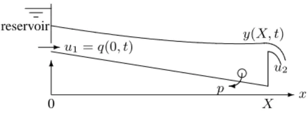
reservoir u1= q(0, t) u2 -¾ p y(X, t) 6 -x X 0

Fig. 1. Schematic representation of the canal

The experimental canal is a trapezoidal and lined canal, with a general cross section of bottom width 0.15 m, sides slope 1:0.15 (V:H) and depth 0.90 m. The overall canal is 145.5 m long and the average longitudinal bottom slope is about

1.5 × 10−3_{. The design flow is 0.09 m}3_s−1_.

Y0 -¾ T0 P0 6 K ¸

Fig. 2. Section of a trapezoidal canal

There is an offtake p at the downstream end of the pool of the orifice type with additional external pipe, equipped with an electromagnetic flowmeter and a motorized butterfly valve. In order to enable the digital control in real time, a water level sensor is installed within an offline stilling well, at the downstream end of the pool. The sensor is of float and counter-weight type attached by a stainless steel tape; this tape runs

over a sprocket wheel. The wheel movements are transmitted to a potentiometer that transmits to the controller the analog inputs correspondent to the water surface.

The canal inlet is equipped with a motorized flow control

valve, that delivers a discharge u1 with the use of a local

slave controller (the level in the upstream reservoir is also regulated using pumps). The downstream end of the canal pool

is controlled with a rectangular sluice gate u2(overshot gate).

All the numerical and experimental results presented in the paper are based on this canal.

III. MODELLING OF AN IRRIGATION CANAL

We present in this section the linearized Saint-Venant equa-tions, used to obtain a transfer matrix representation of the system. A more detailed description is given in [14]. The considered canal pool is a channel with uniform geometry.

A. Irrational model based on Saint-Venant equations

1) Linearized Saint-Venant equations: The hydraulic

be-havior of an open-channel irrigation canal is well described by the so-called Saint-Venant equations [4], which are hyperbolic nonlinear partial differential equations involving the average discharge Q(x, t) and the water depth Y (x, t) along one space dimension x ∈ [0, X], with X the pool length.

We consider small variations of water depth y(x, t) and

discharge q(x, t) around stationary values Q0(x) = Q0(m3/s)

and Y0(x) (m) defined by the backwater curve equation

dY0(x)

dx =

Sb− Sf 0(x)

1 − F0(x)2

(1)

where Sb is the bed slope, F0 the Froude number F0 = _CV0₀

with V0 the average velocity (m/s) and C0=

q

gA0

T0 the wave

celerity (m/s), with T0the water surface top width (m), A0the

wetted area (m2) and g the gravitational acceleration (m/s2).

Throughout the paper, the flow is assumed to be subcritical,

i.e. F0< 1. Eq. (1) is solved for a given downstream boundary

condition Y0(X), leading to the so-called backwater curve

Y0(x).

The friction slope Sf 0 is modelled with Manning-Strickler

formula [4]: Sf 0(x) = Q 2 0n2 A0(x)2R0(x)4/3 (2)

with n the roughness coefficient (sm−1/3) and R0(x) the

hydraulic radius (m), defined by R0 = A0/P0 where P0 is

the wetted perimeter (m) (see figure 2).

The calibration and validation of the Saint-Venant model on field data is discussed in [17]. The obtained Manning coefficient is n = 0.017, corresponding to the roughness of a concrete-lined channel.

Linearizing the Saint-Venant equations around these station-ary values leads to:

T0∂y ∂t + ∂q ∂x = 0 (3) ∂q ∂t + 2V0 ∂q ∂x− β0q + (C 2 0− V02)T0∂y ∂x − γ0y = 0 (4)

with γ0= V02dTdx0+gT0 £ (1 + κ0)Sb− (1 + κ0− F02(κ0− 2))dY_dx0 ¤ , β0= −2g_V0 ¡ Sb−dY_dx0 ¢ and κ0= 7₃−_3T4A_0P0₀dP_dY0.

The boundary conditions are the upstream and downstream discharges q(0, t) and q(X, t).

2) Linearized Saint-Venant transfer matrix: Using Laplace

transform, one can deduce from equations (3–4) the frequency response of the Saint-Venant equations in terms of a transfer matrix linear model that can be used for control purposes [14]. This model relates the upstream and downstream water elevations to the upstream and downstream discharges of the canal pool: µ y(0) y(X) ¶ = µ p11(s) p12(s) p21(s) p22(s) ¶ µ q(0) q(X) ¶ (5) Figure 3 presents the Bode plots of the continuous models p21(s) and p22(s) for the Évora canal relating the upstream and downstream discharges to the downstream water elevation. Their rational approximations are also plotted on the same graph. The frequency response of the canal shows that it behaves as an integrator for low frequencies. This is coherent with the physical interpretation: the canal is similar to a reservoir whose level varies according to the input discharge.

The transfer p21(s) includes a time-delay, which makes its

phase decrease towards −∞. The system has a non zero gain for high frequencies, expressing a direct influence of the discharges on the water levels, and there are oscillating modes that correspond to the interactions of waves propagating

upstream at speed C0− V0 and downstream at speed V0+ C0

[14]. 10−3 10−2 10−1 −20 −10 0 10 20 30 40 freq.(rad/s) gain (dB) p 21 10−3 10−2 10−1 −1200 −1000 −800 −600 −400 −200 0 freq.(rad/s) phase (dg) 10−3 10−2 10−1 0 5 10 15 20 25 30 35 freq.(rad/s) gain (dB) p 22 10−3 10−2 10−1 80 90 100 110 120 130 140 150 freq.(rad/s) phase (dg)

Fig. 3. Bode plots of the irrational transfer functions p21(s) and p22(s)

(—) for Q0= 45 l/s, Y0(X) = 0.6 m, and their rational approximations (–

–).

We have shown in [14] that the transfer functions obtained from Saint-Venant model have the following inner-outer fac-torization [10]:

p21(s) = p21o(s)e−τ1s p22(s) = p22o(s)

with τ1the time-delay for downstream propagation and where

p21o and p22o are outer.

In the general case, the delay τ1 is obtained as:

τ1=

Z X 0

dx

V0(x) + C0(x) (6)

where C0 is the gravity waves celerity and V0 is the flow

velocity. For the considered experimental canal, the time-delay is equal to 60 s for Q = 45 l/s and a downstream boundary

condition Y0(X) = 0.6 m.

The linear Saint-Venant model needs to be completed with the linearized hydraulic structures equations in order to get the model for control design.

3) Linearized hydraulic structures equations: The

equa-tions describing hydraulic structures interacequa-tions with the flow are linearized and added to the model. The hydraulic structure (over shot gate) is modelled using the linearized equations [13]:

q(X, t) = k1y(X, t) + k2u2(t) (7)

with q(X, t) the discharge through the structure, y(X, t) the

water depth upstream of the structure, u2(t) the gate opening.

Coefficients k1, k2 are obtained by linearizing the structure

equation around a given functioning point, corresponding to the hydraulic stationary regime.

4) Complete linear model: In the following, we denote by

y the controlled water level (downstream of the pool), G1(s)

and G2(s) respectively the transfer functions from u1 and u2

to y, and ˜G(s) the transfer function from the perturbation p

to y. The canal pool is therefore represented by:

y = G1(s)u1+ G2(s)u2+ ˜G(s)p (8)

where y is the downstream water level, u1the upstream control

(the upstream discharge q(0, t)), u2 the downstream control

(the downstream gate opening), and p is the downstream perturbation (corresponding to the unknown withdrawal). p acts as an additive perturbation on the downstream discharge

q(X, t), therefore the transfer function is given by ˜G(s) =

G2(s)/k2, with G1(s) = _1−kp21_1p(s)_22(s) and G2(s) = _1−kk2p₁22_p22(s)_(s).

As shown above, the local transfer G2 (relating the

down-stream control u2 to the output y) is outer, while the distant

one G1 (relating the upstream control u1 to the output y) has

an inner part which is a pure time-delay. This remark, which may seem obvious for hydraulic engineers has important implications in terms of control, as will be demonstrated below.

In a first approximation, a canal pool can be viewed as a delayed integrator. Including the interaction with the hydraulic structure, a simple approximation is therefore:

G1(s) ≈ _Ads+ke−τ1s₁ and G2(s) ≈ −_Ads+kk2 ₁ (9)

where Ad is the inverse sensitivity of the downstream water

level to the input discharge and the time delay is obtained by equation (6).

This simplified model captures the main low frequency characteristics of the system. However, for advanced control methods, it is preferable to have an accurate rational model. Such an approximation can be obtained numerically.

B. Rational model approximation

The difficulties to use the linearized Saint-Venant equations

associated to (5) is mainly linked to the facts that pij(s),

the solutions of (5) are irrational transfer functions and that system (5) has in general not closed-form solution. These two difficulties can be nevertheless bypassed. Indeed, in the one hand, it is possible for any value of s ∈ C to obtain the

numerical value associated to pij(s). Let us note that the

numerical resolution of (5) is not so easy, and thus it has been necessary to develop an efficient algorithm to compute the transfer functions (see [16]). In the other hand, an accurate rational transfer representation of the system in the finite band of frequency is sufficient to control the system. Let us recall that this band of frequency is finite since at least constrained by actuators bandwidth.

Following these two points, the approximation of solution of system (5) leads for example to solve this problem: given a set of frequency response data for specified frequency points, we search a rational approximation with an error as small as possible on a given bandwidth and a fixed upper bound for high frequencies.

This problem is in general difficult to solve. We investigated three different methods:

• When the poles of the system are known, the problem is

a convex optimization, which is easy to solve;

• Since we know the inner part of the transfer functions, we

can approximate the modulus of the transfer functions, and approximate the delay with a Padé approximation. This is still a convex problem, but leads to a higher order for the rational model (see e.g. [27]);

• We can also directly approximate the transfer function

frequency response. This leads to a lower order than the second point, but this is not convex, and the result depends on the initialization point.

Remark 1: The use of Remez type algorithms, classically

used in the filter design (see e.g. [3], [30]) allows for methods 1 and 2 to avoid the difficulties of a priori choice of frequency sampling. Even if it is necessary to evaluate more frequency points in this case, this allows to decrease the numerical difficulties linked to undamped oscillating modes.

We used in this paper the first option, since for a prismatic channel, it is relatively easy to compute the poles of the linearized Saint-Venant equations [14]. The rational model of the canal used in the paper is of order 11, with five oscillating modes (see figure 3). Figure 4 presents the Bode plots of

the continuous models G1(s) relating the upstream discharge

to the downstream water elevation and G2(s) relating the

downstream discharge to the downstream water elevation for a set of discharges, and their rational approximations.

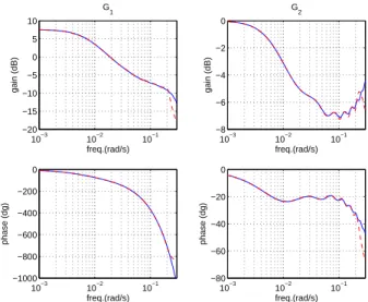
The rational approximations fit very well the linearized Saint-Venant model up to a rather high frequency (0.2 rad/s, corresponding to the fifth oscillating mode).

IV. MIXED CONTROLLER DESIGN

A. Control specifications

A naive analysis of the control problem for irrigation canals would be to consider that the control specifications can be

10−3 10−2 10−1 −20 −15 −10 −5 0 5 10 freq.(rad/s) gain (dB) G 1 10−3 10−2 10−1 −1000 −800 −600 −400 −200 0 freq.(rad/s) phase (dg) 10−3 10−2 10−1 −8 −6 −4 −2 0 freq.(rad/s) gain (dB) G 2 10−3 10−2 10−1 −80 −60 −40 −20 0 freq.(rad/s) phase (dg)

Fig. 4. Bode plots of the continuous models G1(s) and G2(s) (—) and

their rational approximations (– –) for Q0= 45 l/s, Y0(X) = 0.6 m.

reduced to rejecting unmeasured perturbations by controlling the downstream water level. To reduce the problem to this classical control problem leaves apart an essential aspect of the specifications: the water resource management.

As will be shown below, there is a conflict between the wa-ter resource management and the real-time performance with respect to the user. The main issue at stake for irrigation canal control is therefore a better trade-off between these two points. The main objective of the paper is to propose a methodology that gives to the manager the ability to tradeoff between real-time performance and water resource management.

Before presenting our control design method, let us first discuss classical control politics for irrigation canals.

B. Classical control politics vs. specifications

1) Distant downstream control of a canal: Distant

down-stream regulation of a canal pool consists in controlling the downstream water level using the upstream control variable u1. The closed-loop system is given by:

   e = r − y u1 = K1(s)e y = G1(s)u1+ ˜G(s)p

with r the reference water level and e the tracking error. When water is withdrawn from the canal pool, the down-stream level drops, since the downdown-stream discharge is sup-posed to stay constant. Then, the controller reacts by increas-ing the upstream discharge to compensate for this withdrawal, to maintain the downstream water level to its setpoint. In that case, the upstream control variable adapts to the consumed discharge in the pool, therefore uses only the necessary water to satisfy the effective water demand.

The water user sees the real-time performance as the ability of the controller to reject unmeasured perturbations acting in the pool. It is characterized by the modulus of the following transfer function

e = G(s)˜

where S1 is the sensitivity function S1 = (1 + G1K1)−1. The design consists in designing a monovariable controller K1(s) such that |S1(jω)| is minimum on the largest frequency bandwidth.

We recall here an implication of a time-delay in the model. It is well-known that a pure time-delay limits the maximal achievable performance of a controlled system. Let us define the real-time performance of the controlled system as the

highest frequency ωs such as |S1| stays below 1, or:

ωs= max{ω1 : |S1(jω)| < 1, ∀ω < ω1} (11) Following the line of [18] and [12], it can be shown that

ωs≤ π

3τ1

≈ 1

τ1

The downstream control structure is therefore parsimonious in terms of water resource management, but has a limited real-time performance with respect to the user.

2) Local upstream control of a canal: Local upstream

regulation of a canal pool therefore consists in controlling the downstream water level using the downstream control variable

u2. In this case, the closed-loop system is given by:

   e = r − y u2 = K2(s)e y = G2(s)u2+ ˜G(s)p

and the sensitivity is given by

e = G(s)˜

I + G2(s)K2(s)

p = ˜G(s)S2(s)p (12)

When a water withdrawal occurs in the pool, the down-stream level drops. Then, the controller reacts by decreasing the downstream discharge by the amount of the discharge withdrawn. This is possible only if there is enough water flowing downstream (the linear model assumes variations around a given reference flow). Therefore, the local upstream control structure does not link the control to the water resource management: in order to be able to control water levels in this case, one needs to let the maximum discharge flow in the canal (or to constrain the possible withdrawals, by specifying a rotational schedule). The perturbations are always propagated downstream.

Concerning the real-time performance with respect to the user, contrarily to the distant downstream case, there is no

delay in the transfer function G2(s) and no right half-plane

zeros. Then, the achievable bandwidth has no structural limita-tion even if it is in practise limited by the actuators, transmis-sion delays and high frequency dynamic uncertainties. This explains why the local upstream control is more performing than distant downstream control from a monovariable point of view in terms of rejecting downstream perturbations. But this control structure is not satisfactory in terms of water resource management.

C. Multivariable structure: a mixed control politic

The two classical control structures presented above are widely used mainly because they are monovariable control structures, where controller design can be done with classical

tools. We now examine the multivariable control problem,

where both control action variables u1 and u2 are used to

control the downstream water level y. The controller design problem leads to finding a controller K(s) that relates the

tracking error e to the control vector (u1, u2):

K(s) =

µ

K1(s)

K2(s)

¶

Using equation (8), the open-loop transfer matrix is given by:

G(s)K(s) = G1(s)K1(s) + G2(s)K2(s)

Let us now examine the design specifications with respect to the control structure. If the required performance with respect to the user can be satisfied by a distant downstream controller, then there is no need to mix the control methods. However, if the distant downstream controller cannot satisfy the real-time performance specification, it is possible to use the local upstream control for this purpose. It is then necessary to add

a constraint on u2. Since the discharge needs to come from

upstream, we would like to use u2only for transients, and that

in steady state, only u1 has an effect on y.

The control objectives are therefore threefold:

• maintain the downstream water level by rejecting

unmea-sured perturbations induced by water users,

• ensure that the effect of perturbations on the downstream

discharge are only transient,

• ensure robustness with respect to static gain error of

actuators (at least 6 dB of gain margin).

The second objective ensures that, in steady state, a water demand in the pool can only be satisfied by the upstream discharge.

This can be viewed as a problem of actuators substitution, and can be taken into account with an input cascade framework

[32]. The (rapid) upstream control u2 is used to control the

output y:

u2= K2(s)(r − y)

And the (slow) distant downstream control u1 is used to

regulate u2 to a reference ru2 (ru2= 0 in steady state).

u1= K1b(s)(ru2− u2)

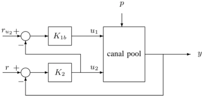
The controller structure can be schematized as in figure 5.

r + − ru2 − - -+ u1 u2 y K2 K1b -canal pool 6 -6 ? p

Fig. 5. Cascade architecture with two control variables (u1, u2) to control

If ru2 = 0, one obtains a multivariable controller as noted

above with K1= −K1bK2.

The advantage of this method is that it decouples the controllers design. One may successively design in such a way two SISO controllers. However, it is generally difficult to specify robustness margins in this case.

We keep a similar structure in the following, but recasting

the problem as an H∞ optimization problem, which can

naturally take into account performance and robustness issues. In our case, we need to ensure robustness with respect to static gain actuators uncertainties, which can be done by ensuring sufficient real input gain margins.

D. Expression of design specifications as H∞ constraints

We propose a multivariable design method using H∞

opti-mization, in order to give a solution to the trade-off between real-time performance and resource management.

Following the approach used in [15], design specifications

are formulated using a H∞ 4-blocks type criterion. Let the

system be described by:

· y u2 ¸ = Ga · u1 u2 ¸ + eGap with Ga= µ G1 G2 0 1 ¶ and eGa= µ e G 0 ¶ .

In order to constrain the downstream control u2 to go

asymptotically to zero, ru2−u2is feed back into the controller

as a tracking error. For usual functioning, ru2 is zero.

There-fore, imposing a low gain in low frequencies for the transfer

function that links the reference ru2 to the error ru2− u2 will

impose a low value for u2 at these frequencies.

The closed-loop system which links the reference ¯r =

[r , ru2]

T _{and the perturbation p to the tracking error ¯e =}

[r − y , ru2− u2]

T _{and the controlled input u = [u}

1, u2]T is given by · ¯ e u ¸ = Ã Sa SaGea KaSa KaSaGea ! · ¯ r p ¸ (13)

where Ka is the controller for the augmented system Ga and

Sa= (I + GaKa)−1is the sensitivity function for system Ga. The design specifications are then formulated using the following criteria, where the goal is to find the smallest γ > 0

and the stabilizing controller Ka such that

° ° ° ° ° Ã W1Sa W1SaGeaW3 W2KaSa W2KaSaGeaW3 !°_° ° ° ° ∞ ≤ γ (14)

with W1 = diag(W11, W12), W2 = diag(W21, W22),

Wik, W_ik−1 ∈ RH∞ and W3 ∈ R is a scaling factor acting

on the perturbation.

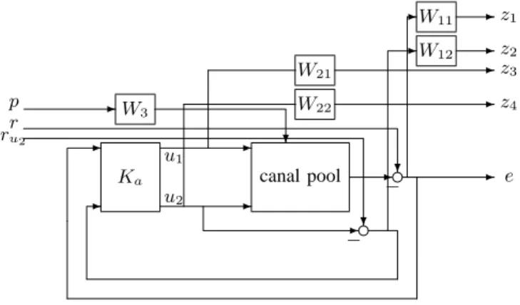
The system augmented with weighting functions is de-scribed in figure 6.

The weighting functions Wik are chosen of the first order.

In order to facilitate the frequency tuning, we use the form proposed by [7], but other forms are available [32]:

Wik(s) =

Gik,∞

q

|G2

ik,0− 1|s + Gik,0ωik,c

q |G2 ik,∞− 1| q |G2 ik,0− 1|s + ωik,c q |G2 ik,∞− 1| -W22 canal pool W11 W3 u2 u1 -e r -W21 -W12 ? -z4 Ka p z3 -? ru2 -−? --z1 z2 -- − -

-Fig. 6. Augmented system for H∞optimization

where _   |Wik(j0)| = Gik,0 limω→∞|Wik(jω)| = Gik,∞ |Wik(jωik,c)| = 1

The performance requirements are easy to specify with these weighting functions:

• W11specifies the overall performance of the system with

respect to the users requirement. This specification has to be compatible with bandwidth constraints associated to the upstream control actuator. The system bandwidth

is closely related to the frequency ω11,c where the gain

of W11 equals 1.

• W12corresponds to the substitution specification between

downstream and upstream actuators. It has to be chosen

in order to be compatible with the time-delay, i.e. ω12,c≤

1/τ1.

• W₂₁ allows to impose roll-off on the upstream control

actuator and it has to be compatible with the substitution

specification associated to W12. Following the chosen

parametrization of the weighting function, ω21,c≈ 10 ×

ω12,c.

• W22 allows to impose strong roll-off on the downstream

control actuator and it has to be compatible with the performance specification associated to W11. Following the chosen parametrization of the weighting function,

ω22,c ≈ 10 × ω11,c. Let us finally note that this roll-off

is necessary in order to avoid any active control of canal oscillating modes by the downstream control actuator. It appears more difficult to directly specify robustness requirements, since the chosen criteria does not explicitly consider robustness constraints. We show below that an input margin constraint can be specified by a careful choice of weighting functions. Let us recall that the input margin is given by [32]: ∆G ∈ · 1 − 1 kTuk∞, 1 + 1 kTuk∞ ¸ [" 1 1 + 1 kSuk∞ , 1 1 − 1 kSuk∞ # (15)

where Su and Tuare the input sensitivity and complementary

In our case, due to the specific structure of the controller, the input sensitivity functions have the following expressions:

Su= Sy µ 1 + G2K2 −G2K1 −G1K2 1 + G1K1 ¶ and Tu= Sy µ G1K1 G2K1 G1K2 G2K2 ¶ with Sy = (1 + G1K1+ G2K2)−1.

Let us evaluate the structured singular value of Tu with

respect to a diagonal complex uncertainty ∆. In the case of a

2 × 2 matrix A, the structured singular value µ∆ is equal to the upper bound [34]:

µ∆(A) = inf

D∈Dσ(DAD

−1₎ with D = {diag(d, 1) : d ∈ R, d > 0}.

After tedious but straightforward manipulations, the

struc-tured singular value of Tu is obtained as:

µ∆(Tu) = |Sy|(|G1K1| + |G2K2|)

We are therefore able very efficiently to impose the input

margin under the parameter G11,∞ of W11, which allows to

constrain Sy, and the parameters G21,∞ of W21 and G22,∞

of W22, which allow to constrain K1 and K2.

The weighting functions are tuned sequentially: first W22is

tuned to specify the maximum bandwidth for local upstream

control, then W11 is tuned to specify the global real-time

performance, then W12 is used to specify the actuators

sub-stitution. W21 and the scaling factor W3 are used to specify

control effort and robustness requirements.

V. EXPERIMENTAL RESULTS

A. H∞ controllers design

Three different H∞ controllers are designed and tested on

the canal, to show the ability of the proposed control scheme to provide a compromise between real-time performance and water management issues. The first controller is a pure distant

downstream controller, where the control action u2 is not

operated, therefore its real-time performance with respect to the user is rather low, as it is limited by the time delay. The

second controller is a mixed controller, using u2to increase the

real-time performance. And the third one is a mixed controller with a high real-time performance, close to the one obtained by a pure local upstream controller. For the three controllers, the optimization resulted in γ ≈ 1. The parameters for the weighting functions of the three controllers are given in tables

I–III. The parameter ωc for weighting function W11 gives

a good approximation of the controlled system bandwidth.

This parameter is increased from 5 × 10−3 rad/s for the first

controller to 2.5 × 10−2 rad/s for the second, and 5 × 10−2

rad/s for the third controller, i.e. 10 times the bandwidth of the first one. This illustrates the ability of the control scheme to “tune” the real-time performance with respect to the user.

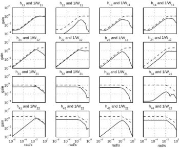
Figure 7 presents the transfer functions appearing in the

H∞criteria with associated constraints for controller 2. Each

transfer is indeed below the associated constraint, showing that the obtained γ is smaller than 1.

TABLE I

PARAMETERS OF THE WEIGHTING FUNCTIONS,CONTROLLER1

W11 W12 W21 W22 W3

G0 1000 1 0.9 0.5 0.48

G∞ 0.4 0.9 1000 1000

ωc 5 × 10−3 rad/s 5 × 10−5 rad/s 10−2 rad/s 10−5 rad/s

TABLE II

PARAMETERS OF THE WEIGHTING FUNCTIONS,CONTROLLER2

W11 W12 W21 W22 W3

G0 1000 10000 0.9 0.2 0.69

G∞ 0.8 0.2 1000 1000

ωc 2.5 × 10−2 rad/s 5 × 10−3 rad/s 10−2 rad/s 10−1 rad/s

Figure 8 depicts the singular values of the three controllers. It is clear that the first controller uses only one control input (corresponding to the distant downstream control politics) and controller 3 has a larger bandwidth than controller 2.

This better real-time performance is obtained to the expense of some robustness. Indeed, let ∆G denote the real multi-variable gain margin (static gain margin). Using eq. (15), we obtain:

∆Gmin≤ ∆G ≤ ∆Gmax

with ∆Gmin and ∆Gmax given in table IV for the three

controllers.

The controllers have been obtained with the robust control toolbox of Matlab. The order of the controllers is 15, i.e. the order of the system augmented by the order of the weighting functions. The controllers have been discretized at a sampling time 0.125 s, and we used a balanced realization for implementation. 10−4 10−2 100 102 gain

h₁₁ and 1/W₁₁ h₁₃ and 1/W₁₁ h₁₄ and 1/W₁₁

10−4 10−2 100 102 gain h₂₁ and 1/W₁₂ 10−4 10−2 100 102 gain 10−6 10−4 10−2 100 10−4 10−2 100 102 rad/s gain 10−6 10−4 10−2 100 rad/s 10 −6 10−4 10−2 100 rad/s 10−6 10−4 10−2 100 rad/s h₂₃ 1/W₁₂ h₁₁ 1/W₁₁ gain gain rad/s h₁₂ and 1/W₁₁

h₂₂ and 1/W₁₂ h₂₃ and 1/W₁₂ h24 and 1/W12

h31 and 1/W21 h32 and 1/W21 h33 and 1/W21 h34 and 1/W21

h₄₁ and 1/W₂₂ h₄₂ and 1/W₂₂ h₄₃ and 1/W₂₂ h₄₄ and 1/W₂₂

Fig. 7. Closed loop transfer functions (—) and associated inverse frequency weighting functions (– –) for controller 2. hijdenotes the transfer between the jthinput and the ithoutput of the augmented system used in the H∞ criteria (14).

TABLE III

PARAMETERS OF THE WEIGHTING FUNCTIONS,CONTROLLER3

W11 W12 W21 W22 W3

G0 1000 10000 0.9 0.2 0.34

G∞ 0.8 0.2 1000 1000

ωc 5 × 10−2 rad/s 5 × 10−3 rad/s 2 × 10−2 rad/s 2 × 10−1 rad/s

10−5 ₁₀−4 ₁₀−3 ₁₀−2 ₁₀−1 ₁₀0 ₁₀1 −120 −100 −80 −60 −40 −20 0 20 40 60 Singular Values Frequency (rad/sec) Singular Values (dB)

Fig. 8. Singular values of controller 1 (. . . ), controller 2 (– –) and controller 3 (—)

B. Experimental results

We now compare the three controllers tested on the real canal, with the same scenario: an unpredicted downstream withdrawal of 10 l/s stopped after stabilization.

Figure 9 gives the experimental results obtained with the

distant downstream H∞ controller 1. A downstream

with-drawal of 10 l/s (0.01 m3/s) is done at time t = 20 s and

stopped at time t = 700 s. In that case, the downstream action variable is not operated, and only the upstream discharge is used to compensate for the water withdrawal.

Figure 10 gives the experimental results obtained with the

mixed H∞ controller 2. The downstream outlet is opened at

time t = 110 s and stopped at time t = 650 s. The controller reacts as expected: first the downstream overshot gate is closed

in order to maintain the output y at the target yc = 0.6 m,

then occurs the substitution with the upstream control; the downstream gate opens gradually while the upstream discharge increases in order to compensate for the withdrawal. In steady state (between 300 and 900 s), the upstream discharge is 10 l/s higher than the initial one, which corresponds exactly to the withdrawal. This ensures that the water needed downstream comes from the resource, located upstream, and is not taken from the water needed downstream.

Figure 11 gives the experimental results obtained with the

TABLE IV

ROBUSTNESS MARGIN OF THE THREE CONTROLLERS

Controllers 1 2 3

∆Gmin(dB) −∞ -5 -4.2

∆Gmax(dB) 10.2 8.8 8

mixed H∞ controller 3. The downstream outlet is opened at

time t = 150 s and stopped at time t = 850 s. Here also, the controller reacts as expected, and quicker than the mixed controller 2.

The multivariable H∞controllers enable to recover the

real-time performance of a pure local upstream controller while ensuring that in steady state, the discharge is delivered by the upstream control (as for a distant downstream controller). In addition, one observes that the linear simulation reproduces rather accurately the dynamic behavior of the closed-loop sys-tem. The main discrepancy concerns the downstream actuator u2, which has a 2 mm dead band which is not modelled here. This, together with the important measurement noise explains the differences between the experiment and the simulation. The response times are however very close and the controller reacts as expected. 0 200 400 600 800 1000 1200 0.58 0.59 0.6 0.61 0.62 time (s) water depth (m) Mixed H ∞ control 0 200 400 600 800 1000 1200 0.045 0.05 0.055 0.06 time (s) discharge (m 3/s) 0 200 400 600 800 1000 1200 0.36 0.38 0.4 0.42 0.44 0.46 time (s) gate opening (m) measured u2 simulated u2 measured u1 simulated u1 measured y simulated y

Fig. 9. Experimental response of the distant downstream H∞controller 1 to a downstream withdrawal, comparison with a linear simulation

0 100 200 300 400 500 600 700 800 900 1000 0.58 0.59 0.6 0.61 0.62 time (s) water depth (m) Mixed H_∞ control 0 100 200 300 400 500 600 700 800 900 1000 0.045 0.05 0.055 0.06 time (s) discharge (m 3/s) 0 100 200 300 400 500 600 700 800 900 1000 0.36 0.38 0.4 0.42 0.44 0.46 time (s) gate opening (m) measured y simulated y measured u1 simulated u1 measured u2 simulated u2

Fig. 10. Experimental response of the mixed H∞ controller 2 to a

downstream withdrawal, comparison with a linear simulation

Finally, the proposed solution appears to stabilize a large set of stationary linearizations of the canal. This is not surprising,

0 200 400 600 800 1000 1200 0.58 0.59 0.6 0.61 0.62 time (s) water depth (m) Mixed H_∞ control 0 200 400 600 800 1000 1200 0.045 0.05 0.055 0.06 time (s) discharge (m 3/s) 0 200 400 600 800 1000 1200 0.36 0.38 0.4 0.42 0.44 0.46 time (s) gate opening (m) measured y simulated y measured u1 simulated u1 measured u2 simulated u2

Fig. 11. Experimental response of the mixed H∞ controller 3 to a

downstream withdrawal, comparison with a linear simulation

since the change of functioning point has a slow dynamics in the case of a canal. Therefore, the gain scheduling heuristic is fulfilled: the parameters defining the linearizations vary very slowly compared to the system’s dynamics [8]. This is coherent with a widespread engineers’ practice, using gain-scheduling heuristics to design efficient controllers.

C. Performance indicators

The controllers’ performance is evaluated using various indicators. The real-time performance is evaluated using clas-sical indicators, the Integrated Absolute Error (IAE) and the Maximum Absolute Error (MAE), defined as follows:

IAE =100 T R_T 0 |y(t) − yc|dt yc and M AE = 100max[0,T ](|y(t) − yc|) yc

where yc is the setpoint for the downstream water elevation.

These indicators are dimensionless, and evaluate the real-time performance of the control system: the lower they are, the better the system is controlled. Indeed, these indicators evaluate the performance of the control, in terms of water delivery: the lower they are, the better the water users’ demand is satisfied, since the delivered discharge is directly linked to the downstream water level for gravity offtakes.

The water management is evaluated using two indicators, the Water Efficiency (WEF)

W EF = 100

RT 0 qp(t)dt

RT 0 q1(t)dt

where q1 is the upstream discharge of pool 1 and qp the

dis-charge delivered to the outlet, and the Maximum Downstream Perturbation (MDP)

M DP = 100max[0,T ](q2(t))

max[0,T ](q1(t))

where q2 is the upstream discharge of pool 2, i.e. the

down-stream discharge of pool 1.

These indicators are also dimensionless. The Water Effi-ciency evaluates the volume of water delivered to the outlet relatively to the volume of water taken from the upstream reservoir. The closer this indicator is to 100, the better the water management.

The Maximum Downstream Perturbation indicator evaluates the impact of the first pool on the other pools downstream. If this indicator is higher than 100, it means that the control system generates higher discharge perturbations than it is necessary.

These indicators are computed for the three controllers. Results are given in table V.

TABLE V

PERFORMANCE INDICATORS FOR THE THREE CONTROLLERS

Controllers 1 2 3

IAE 1.23 0.50 0.25

MAE 3.33 2.0 1.61

WEF 78.85 91.51 87.20

MDP 92.8 101.6 105.8

As could be expected, the “best” controller in terms of real-time performance is the controller 3 since it has an IAE of 0.25, which is twice better than controller 2, and 5 times better than controller 1. The MAE for controller 3 is close to the best achievable real-time performance, taken into account actuators and sensors limitations.

Also, this very good real-time performance induces a good water management, since the Water Efficiency is much higher for controllers 2 and 3 than for controller 1. The WEF is slightly lower for controller 3 than for controller 2 because of the system nonlinearity: due to the dead-band in the downstream actuator, the system final steady state necessitated a higher input discharge to match with the downstream water elevation. This supplementary discharge has lowered the Water Efficiency indicator for controller 3.

The use of the downstream actuator induces larger pertur-bations propagated downstream, compared to the controller 1. The perturbation are amplified with controller 3 (105.8 %, corresponding to an amplification of about 6 %) and the amplification is more limited for controller 2 (101.6 %). In the case of controller 1, the perturbation is attenuated, but part of the perturbation affects the water delivery.

Depending on the downstream canal pool hydraulic charac-teristics, this amplification can be attenuated when propagating downstream. Therefore, the choice between these controllers has to be done by the manager, according to his objectives and to the canal characteristics.

In conclusion, the manager can choose between these con-trollers the one suited for the specific canal control problem. The proposed method enables to easily obtain a controller from

a classical H∞ optimization.

VI. CONCLUSION

The paper has exposed and validated a method to design efficient automatic controllers for an irrigation canal pool, that

realize a compromise between the water resource manage-ment and the performance in terms of rejecting unmeasured perturbations. This mixed controller design is casted into the

H∞ optimization framework, and experimentally tested on a

real canal located in Portugal. Classical control politics for an irrigation canal (local upstream and distant downstream control) have been interpreted using automatic control tools. The proposed mixed control politics enables to combine both classical politics, keeping the distant downstream control water management while recovering the local upstream control real-time performance with respect to the user. Such a design method gives to the manager a tool to balance the trade-off by using the multivariable feature of the controller.

To the best of the authors’ knowledge, this paper is among

the first applications of H∞ control to a real canal. It opens

interesting perspectives for the modernization of irrigation canals management. Ongoing research deals with the problem of controlling multiple canal pools using a similar approach.

ACKNOWLEDGMENTS

This work was partially supported by the French Embassy in Portugal and GRICES (Gabinete de Relações Internacionais da Ciência e do Ensino Superior) of Portugal, through the

collaboration project n◦ 547-B4. We thank Prof. Manuel Rijo

from the University of Évora for the opportunity he gave us to use the canal, and for his hospitality during our stays in Portugal.

The authors acknowledge the financial help of Cemagref and INRA through the collaborative program ASS AQUAE

n◦ 2.

We thank Gérard Scorletti for his help concerning the rational approximation.

REFERENCES

[1] O. Begovich and R. Ortega. Adaptive head control of a hydraulic open channel model. Automatica, 25(1):103–107, 1989.

[2] C.M. Burt and S.W. Styles. Modern water control and management practices in irrigation. Technical report, FAO, IPTRID, World Bank, 1999.

[3] E. W. Cheney. Introduction to approximation theory. American

Mathematical Society, 2nd edition, 2000.

[4] V.T. Chow. Open-channel Hydraulics. McGraw-Hill Book Company, New York, 1988. 680 p.

[5] J.M. Coron, B. d’Andrea Novel, and G. Bastin. A Lyapunov approach to control irrigation canals modeled by Saint-Venant’s equations. In

In-ternational European Control Conference ECC’99, Karlsruhe, Germany,

1999.

[6] J. de Halleux, C. Prieur, J.-M. Coron, B. d’Andéa Novel, and G. Bastin. Boundary feedback control in networks of open-channels. Automatica, 39:1365–1376, 2003.

[7] S. Font. Méthodologie pour prendre en compte la Robustesse des

systèmes asservis : optimisation H∞ et approche symbolique de la forme standard. Ph.D. thesis, Université de Paris-Sud Orsay, France,

1995.

[8] V. Fromion and G. Scorletti. A theoretical framework for gain schedul-ing. Int. J. of Robust and Nonlinear Control, 13:951–982, 2003. [9] D. Georges and X. Litrico. Automatique pour la gestion des ressources

en eau. Information, Commande, Communication. Hermès Science Editions, Paris, 2002.

[10] K. Hoffman. Banach Spaces of Analytic Functions. Prentice Hall,

London, 1962.

[11] H. Jreij. Sur la régulation des cours d’eau aménagés. Ph.D. thesis, Université Paris-XI Dauphine, 1997. (in French).

[12] P.P. Khargonekar and K. Poolla. Robust stabilization of distributed systems. Automatica, 22(1):77–84, 1986.

[13] A. Lencastre. Hydraulique générale. Eyrolles, SAFEGE, 1996. (in French).

[14] X. Litrico and V. Fromion. Infinite dimensional modelling of open-channel hydraulic systems for control purposes. In 41st Conf. on Decision and Control, pages 1681–1686, Las Vegas, 2002.

[15] X. Litrico and V. Fromion. Real-time management of multi-reservoir hydraulic systems using H∞ optimization. In IFAC World Congress, Barcelona, 2002.

[16] X. Litrico and V. Fromion. Frequency modeling of open channel flow.

J. Hydraul. Engrg., 130(8):806–815, 2004.

[17] X. Litrico, V. Fromion, J.-P. Baume, C. Arranja, and M. Rijo. Exper-imental validation of a methodology to control irrigation canals based on Saint-Venant equations. Control Engineering Practice, 13(11):1425– 1437, 2005.

[18] X. Litrico, V. Fromion, and G. Scorletti. Improved performance for open-channel hydraulic systems using intermediate measurements. In

IFAC Workshop on Time-Delay Systems, pages 113–118, Santa Fe, 2001.

[19] X. Litrico and D. Georges. Robust continuous-time and discrete-time flow control of a dam-river system (I): Modelling. Applied Mathematical

Modelling, 23(11):809–827, 1999.

[20] X. Litrico and D. Georges. Robust continuous-time and discrete-time flow control of a dam-river system (II): Controller design. Applied Mathematical Modelling, 23(11):829–846, 1999.

[21] P.-O. Malaterre. Pilote: linear quadratic optimal controller for irrigation canals. J. Irrig. Drain. Engrg., 124(4):187–194, July/August 1998. [22] P.-O. Malaterre and M. Khammash. `1 controller design for a

high-order 5-pool irrigation canal system. Journal of Dynamic Systems, Measurement, and Control, 125(4):639–645, December 2003.

[23] Iven Mareels and Erik Weyer. Systems engineering design for irrigation systems. In IFAC LSS Symposium, 2004. Plenary contribution. [24] M. Papageorgiou and A. Messmer. Continuous-time and discrete-time

design of water flow and water level regulators. Automatica, 21(6):649– 661, 1985.

[25] M. Papageorgiou and A. Messmer. Flow control of a long river stretch.

Automatica, 25(2):177–183, 1989.

[26] P. Pognant-Gros, V. Fromion, and J.P. Baume. Canal controller design: a multivariable approach using H∞. In European Control Conference, pages 3398–3403, Porto, 2001.

[27] L. R. Rabiner, N. Y. Graham, and H. D. Helms. Linear programming design of IIR digital filters. IEEE Trans. on Acoustics, Speech, and

Signal Processing, 22(2):117–123, April 1974.

[28] S. Sawadogo, P.-O. Malaterre, and P. Kosuth. Multivariable optimal control for on-demand operation of irrigation canals. International J. of

Systems Science, 26(1):161–178, 1995.

[29] J. Schuurmans. Control of water levels in open-channels. Ph.D. thesis, ISBN 90-9010995-1, Delft University of Technology, 1997.

[30] I. Selesnick, M. Lang, and C. S. Burrus. Magnitude squared design of recursive filters with Chebyshev norm using a constrained rational Remez algorithm. In 6th IEEE DSP Workshop, 1994.

[31] M.J. Shand. Automatic downstream control systems for irrigation canals. Ph.D. thesis, University of California, Berkeley, 1971.

[32] S. Skogestad and I. Postlethwaite. Multivariable Feedback Control. Analysis and Design. Wiley, 1998.

[33] C.Z. Xu and G. Sallet. Proportional and integral regulation of irrigation canal systems governed by the St Venant equation. In International

Conf. on Systems, Man and Cybernetics, SMC’98, pages 3891–3896,

San Diego, 1998.

[34] K. Zhou and J.C. Doyle. Essentials of robust control. Prentice Hall, Upper Saddle River, NJ 07458, 1998.