A generalized diffusion based inter-iteration nonlinear bilateral filtering scheme for PET image reconstruction.

HAL Id: inserm-00195427

https://www.hal.inserm.fr/inserm-00195427

HAL is a multi-disciplinary open access archive for the deposit and dissemination of sci-entific research documents, whether they are pub-lished or not. The documents may come from teaching and research institutions in France or abroad, or from public or private research centers.

L’archive ouverte pluridisciplinaire HAL, est destinée au dépôt et à la diffusion de documents scientifiques de niveau recherche, publiés ou non, émanant des établissements d’enseignement et de recherche français ou étrangers, des laboratoires publics ou privés.

A generalized diffusion based inter-iteration nonlinear

bilateral filtering scheme for PET image reconstruction.

Jian Zhou, Hongqing Zhu, Huazhong Shu, Limin Luo

To cite this version:

Jian Zhou, Hongqing Zhu, Huazhong Shu, Limin Luo. A generalized diffusion based inter-iteration nonlinear bilateral filtering scheme for PET image reconstruction.. Computerized Medical Imaging and Graphics, Elsevier, 2007, 31 (6), pp.447-57. �10.1016/j.compmedimag.2007.04.003�. �inserm-00195427�

A Generalized Diffusion Based Inter-Iteration

Nonlinear Bilateral Filtering Scheme for PET

Image Reconstruction

Jian Zhou1,2,3,4, Hongqing Zhu5, Huazhong Shu1,4, Limin Luo1,4 1

Laboratory of Image Science and Technology, Southeast University, Nanjing, China 2

INSERM U642, France 3

Universite de Rennes 1, LTSI, Rennes, France 4

Centre de Recherche en Information Biomedicale Sinograncais (CRIBs), France 5

East China Univeristy of Science & Technology, Shanghai, China

HAL author manuscript inserm-00195427, version 1

HAL author manuscript

Abstract

In this paper, a new inter-iteration filtering scheme based diffusion MAP estimate for PET image

reconstruction is proposed. This is achieved by gaining the insights into the classical MAP iteration (e.g.

the OSL algorithm) and the several well-established approximations to the diffusion process. We show that

such a new technique in turn allows additional insight and sufficient flexibility to further investigate some nonlinear filters based reconstruction algorithms. In particular, upon unraveling the limitations but

maintaining the advantages of diffusion regularized method, we suggest the bilateral filter as a nice

application in which image smoothing while edge preserving can be readily obtained by the nice

combination of the range and domain filters. The feasibility and efficiency of the proposed method are

verified in the substantiating experiments conducted on both the computer simulated and real clinical data.

Keywords: image reconstruction, inter-iteration, filtering, MAP, OSL, diffusion, bilateral, range filter,

domain filter.

1. Introduction

Positron emission tomography (PET) is one of the most important imaging tools in modern diagnosis; it

provides valuable information on the biochemical and biological activity inside a living subject in a

non-invasive way. Reconstruction of PET scan images is a complex problem; many algorithms such as

analytic and iterative algorithms have been developed in the past decades to solve this problem. Among iterative algorithms, the statistical reconstruction has become increasingly popular due to its ability to

model the noise and the imaging physics and to impose the positivity constraints on the reconstruction.

As it is well known, PET is an ill-posed problem; that is, small variations in the data produce large

variations in the solution. When using an iterative algorithm, the ML problem in particular, as the likelihood increases, the image starts deteriorating; the algorithm enforces consistency with data, and,

because of the size of the problem, more and more high frequencies related to noise show up. So, iterations

should be stopped before this happens, by using a suitable stopping criterion [1]. A better approach to

overcome the ill-posedness effects is to consider prior information through regularization terms allowing

more sophisticated and accurate models.

Bayesian methods known as the Maximum a Posteriori (MAP) estimate for PET image reconstruction and

restoration have become increasingly popular because they allow accurate modeling of both data collection

and image behavior. The MAP algorithm can remove the divergence in quantitative accuracy at higher

iteration numbers, which is often seen in ML due to noise. The result is often a smoother image in the same

number of iterations. This attributes largely to the introduction of image priori that maintains the

reconstruction without being degenerated by the noise. As for the design of priori, the Gibbs distribution is

commonly used due greatly to its simplicity and well-established rationale. In the past decades, a variety of

prior distributions have been proposed, typically [2], [3], [4], most of which are distinguished by the choice

of energy function in the modeling of Gibbs priori. Recently, the diffusion based priori seems especially attractive in case of tomography reconstruction [5]-[8]. It is mainly because the diffusion techniques

provide a promising way of image denoising while edge preservation. One may readily construct the

diffusion priori by replacing the energy function in the canonical Gibbs distribution with proper gradient

based energy functional. Such an insight has led to the inherent deep connections between the MAP

estimate and the variational partial differential equations (PDE) based anisotropic diffusion progress [9]. As for the anisotropic diffusion, it has played an important role in signal and image analysis since Perona and

Malik's landmark work [10] in which they firstly aimed at persevering sharp features such as edges in

images based on nonlinear evolution equation. Their technique may be more simply interpreted as a

nonlinear filter whose selective smoothing is based upon the computed local gradient. This promising

approach has triggered a tremendous research activity in computer vision and applied mathematics and has been proven to be a powerful tool for restoration and reconstruction of high-quality images.

In this paper, our plan is hence to detail the utilities of nonlinear filtering and help us provide an alternative

view of the problem of PET image reconstruction. This, in turn, will be instrumental in our development of

an alternative interpretation of existing reconstruction methods, e.g., the 'one-step-late' (OSL) algorithm [3], and in using the gained insight to propose the inter-iteration filtering (IIF) scheme to some of the well

known limitations. More specifically, we view the reconstruction as a solution to a controlled iteratively

prediction/correction system. This ultimately leads to an inter-iteration filtering with two typical filters, the

reconstruction filter and the nonlinear filter, well adapted to preserving salient features of images (such as

edges) while smoothing away the noise. In doing so, we furthermore introduce the bilateral filter [11] as a

nice candidate for the nonlinear filter which enables us to distinguishes noise from signal based on not only the amplitude differences of windowed pixels but also on the spatial size of a detail.

The rest of paper is organized as follows: In section 2, we first briefly outline the problem of PET

reconstruction and then introduce the anisotropic diffusion which connects the diffusion based priori and

gives us insights to derive accordingly the new reconstruction algorithm based on the IIF scheme; The corresponding evaluations through both the computer simulated and the real clinical data based examples is

provided in Section 3. Finally, Section 4 gives out some concluding remarks.

2. Methodology

2.1 PET Image Reconstruction

In PET, the isotope used emits positrons which annihilate with nearby electrons generating two photons

traveling away from each other in opposite direction. The emission of positrons is modeled as a spatial,

inhomogeneous Poisson process with unknown intensity, the mean of which is determined by the concentration of the isotope that we wish to estimate. For the convenience of illustration, we assume the

image to be reconstructed is subdivided into J× J pixels and also assume that the activity concentration within each pixel is uniform, denoted by . The data consists of photon coincidence

counts collected by

j f_j

Idetector pairs, Yi,i=1,2,...I. is a sample from a Poisson distribution whose

expectation value is i Y

∑

( Af , where Y is the Poisson random variable corresponding i

to and the element of the projection matrix , is the probability that a positron

emitted from pixel results in a coincidence at the th LOR, is the image vector, i.e., .

The conditional probability of obtaining the measurement vector given the image vector (i.e., the

likelihood function) is i Y A={a_ij}∈ℜI×J aij j i f f =[f₁, ,f_J]T Y f

(

)

∏

The ML method which estimates that maximizes subject to nonnegative constraints on , or,

equivalently, finds the which maximizes

f Pr(Y|f) f 0 ≥ f

{

}

∑

With the help of EM algorithm, Shepp and Vardi proposed the following image update formula for the ML

solution (ML-EM algorithm) [12]:

∑

∑

The ML solution is dominated by noise artifacts, and iterative estimates exhibit increasing noise artifacts

along iterations. Therefore regularization techniques are usually needed to produce a reasonable reconstruction. The Bayesian approach as well as the MAP estimate represents a more complete and elegant

way to stabilize the ML problem by using prior information contained in a regularization term. That is instead of maximizing the likelihood (1), is maximized, i.e., via the Bayesian formula, the new

model becomes ) | Pr(f Y ) Pr( ) | Pr( ) Pr( ) Pr( ) | Pr( ) | Pr( max 0 Y Y f f f f Y Y f f≥ = ∝ (4)

where and are the probabilities of and respectively. A common Bayesian priori is the

Gibbs distribution of the form:

) (f P P(Y) f Y )) ( exp( ) Pr(f ∝ −βΨf , β >0 (5)

where is the so-called energy function. By substituting (5) and (1) into (4) and then taking

logarithm, we obtain the MAP estimate:

) (f Ψ

{

}

One EM-type approach to construct MAP reconstruction has been recommended by Green [3], which is known as the OSL algorithm. In this algorithm, the influence of prior term is only performed at the current

estimate , and thus results in the simple updating equation [3]: fˆ k f

∑

∑

Apparently such an influence is imposed by the meaning of the gradient of the energy function

evaluated at each iteration k . Due to this "one step late" property of this algorithm, a fully iteration can be

interestingly seen as an error prediction/correction technique. Calculation of the priori influence, i.e., the gradient of corresponds to the error prediction, and their use in (7) to reestimate is correction.

In the proceeding the similar technique will be given new interpretations in our proposed algorithm.

) (f U ) (f Ψ fj

2.2 Reconstruction Using Inter-Iteration Filtering Scheme

A. Anisotropic Diffusion

In this section, we will discuss the usage of the nonlinear filter for the problem of PET image reconstruction.

It is necessary to review some basic relations between the anisotropic diffusion process and the underlying nonlinear filtering problem. Let us first consider the following energy functional defined on the spaces of smooth images, that is, images for which ∇f is finite in Ω, as in the following respect to image function

:

f

∫

=

Ψ(f) ρ(|| f ||)d ₍₈₎

where ρ(||∇f ||)≥0 is an increasing function of ||∇f ||. One way we can minimize the above expression

is by means of gradient descent by using the calculus of variations theory which leads to the parabolic PDE: ⎥ ⎦ ⎤ ⎢ ⎣ ⎡ ∇ ∇ ∇ = Ψ = ∂ ∂ f f f div t t y x f || || ||) (|| ' ' ) , , ( ρ (9)

with the initial and boundary conditions:

0 ) 0 , , (x y f f = , and =0 ∂ ∂ Ω ∂ N f (10)

where div(⋅) denotes the divergence operator and N the outward unit norm of the boundary ∂Ω.

By defining

x x x

g( )≡ρ'( ) (11)

and substituting it into (9) we obtain

] ||) (|| [ ) , , ( f f g div t t y x f ∇ ∇ = ∂ ∂ (12) which amounts to Perona and Malik's anisotropic diffusion equation [10]. Function g(⋅) is the so-called

edge-stopping function that is a nonnegative monotonically decreasing function with . The

diffusion process will mainly take place in the interior of regions, and it will not affect the region boundaries where the magnitude of gradient of is large. Qualitatively, the effect of anisotropic diffusion

is to smooth the original image while preserving brightness discontinuities. This is well controlled by the choice of that greatly affects the extent to which discontinuities are preserved.

0 . 1 ) 0 ( = g f ) (⋅ g

Equation (12) can be discretized as follows [13]:

j p j p j k j k j f g f f f 1 ( _, ) _, | | ∇ ∇ + = + η λ (13) where is the discretely sampled image, denotes the pixel position in a discrete 2D grid, and

denotes discrete time steps (iterations). The constant is a scalar that determines the rate of diffusion,

j

f j

k λ∈ℜ+

η represents the spatial neighborhood of pixel , and j |η is the number of neighbors (usually _j|

four). The image gradient is linearly approximated in a particular direction as

k j k p j p f f f = − ∇ , , p∈ηj (14)

Barash and Comaniciu recently noted that the nonlinear diffusion is common with the generalized adaptive smoothing [14], [15]:

∑

∑

where the window Sj covers a local filter support of size(2n+1)×(2n+1),n=1,2, , centered at the

pixel and 's acting as the smoothing kernel correspond to different neighbor combinations with

respect to the center pixel of interest. Typically one can choose as

j w_p

p

w w_p ≡g(∇f_{p, j}) which results in

the fundamental link between the anisotropic diffusion and the edge-preserving smooth filters. In the next subsection, we shall give out more details on the design of filter . It is noted that in practice, need

not be taken too large (usually ), otherwise the generalized adaptive smoothing becomes an inaccurate

representation of the extended diffusion equation which causes the image being oversmoothed [15].

p

w n

3 ≤ n

B. Inter-Iteration Filtering Scheme

The diffusion based MAP reconstruction is to consider the continuous prior probability density as follows

[9]: } ||) (|| exp{ ) Pr(

∫

To approach the corresponding estimate based on the above priori, we can use the insights gaining from the OSL algorithm that is equivalent to solve the gradient of Ψ(f), or more specifically,

j j f ' ) ( _{≅ Ψ} ∂ Ψ ∂ f (17) where F _jdenotes the jth sample of continuous function F. One may reach (17) by properly

discretizing as well as the divergence operator in (2), which usually involves the finite difference to the first and second order partial derivatives and possibly becomes complicated with the different choices of

' Ψ

) (⋅

ρ . However, by noticing the relations between the anisotropic diffusion (13) and the generalized adaptive smoothing (15), we may instead approximate (17) by using the following slightly abusive form

k j j k j S p p S p p p j f w w f f f f f f f = ∈ ∈ = ⎪_⎭ ⎪ ⎬ ⎫ ⎪ ⎩ ⎪ ⎨ ⎧ − ⎟ ⎟ ⎟ ⎠ ⎞ ⎜ ⎜ ⎜ ⎝ ⎛ ≅ ∂ Ψ ∂

∑

∑

Clearly such an approximation is easier to manipulate since it depends only on the choice of smoothing

kernel . Secondly, perhaps the most importantly, because the first term on the right-hand side of (18) acts

like the nonlinear filtering carried on a local structure of the current estimate , it thus can be treated

independently. Therefore, it is worthy to note that (18) does indicate how the reconstruction can be

reinterpreted as an inter-iteration filtering scheme.

p w

j

S fk

More precisely, by substituting (18) into the OSL formula (7), we can present the new algorithm as follows:

∑

∑

where represents the edge-preserving smooth filter at iteration and for each we

typically have k H k j=1, ,J

∑

∑

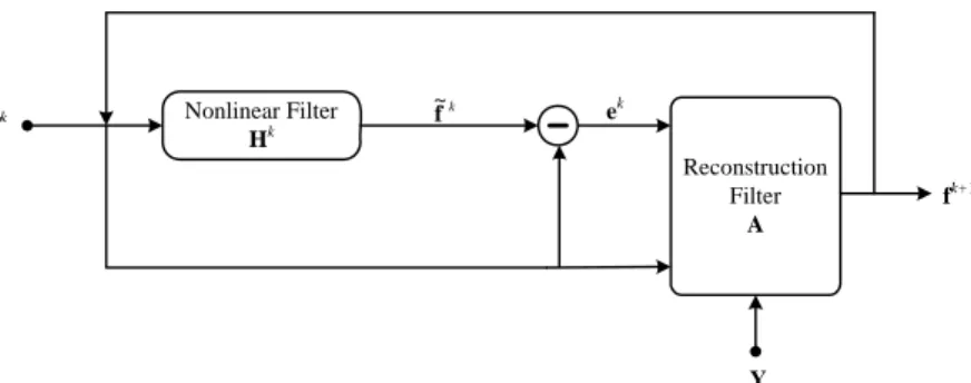
The above iteration scheme furthermore can be summarized in Fig.1.

FIGURE 1

In Fig.1, we describe the reconstruction in the notation of filtering which is also in the spirits of OSL's

prediction/correction technique. Given current estimate , the is obtained by inputting to the nonlinear filter . The output is then subtracted by to produce the residue error which along with

the and observation feeds back to the reconstruction filter to yield the new estimate .

k f _f~k _fk k H _fk _ek k f Y _fk+1

C. Bilateral Filter

Comparing most other diffusion based MAP algorithms, e.g., [6]-[8], the proposed algorithm treats the

diffusion based a priori more implicitly so that we can focus only on the design of smooth filter as well as the weights 's. As mentioned previously, can be taken as and then lead to the

common diffusion filter. However such a filter usually does not consider the pixel position information but emphasize only on their differences to the center pixel of the specific local structure . Thus the effects of

spatial resolution are often ignored and can not be well maintained for the case of practical uses.

k H p w wp g(∇fp, j) j S

One way out of this problem is to model the spatial resolution together with the mentioned diffusion filter

which results in the bilateral filter. The bilateral filtering was first introduced in [11] as the nonlinear filter

which combines domain and range filtering. It has proven to be useful in the accomplishment of compute vision tasks [16], [17] and its nice properties have been well established in several literatures, such as [11], [18], [19], [20]. Given an input image , using a continuous representation notation as in [11], the output

image f f ~ is obtained by

∫ ∫

∫ ∫

where x=(x,y), ξ=(ξ1,ξ2)are space variables. Clearly the convolution kernel is the product of the

functions c ands, which represent ‘closeness’ (in the domain) and ‘similarity’ (in the range), respectively. In case of discrete image, each weight within the specific window Sj then can be determined by

) , ( ) , ( p j p c p j s f f w = . ₍₂₂₎

More specifically, c(⋅,⋅) is usually radially symmetric, taking the Gaussian like function for example [11], ⎟ ⎟ ⎠ ⎞ ⎜ ⎜ ⎝ ⎛ − = ₂ 2 2 ) , ( exp ) , ( D j p d j p c σ (23) where j p j p d j p d( , )= ( − )= − (24)

is the Euclidean distance between pixel pand j, σ denotes the geometric spread controlling the shape D

of Gaussian function. In such a case, we found that the function c(⋅,⋅) acts more like the point spread

function (PSF) of a typical imaging system. Therefore, σ can be similarly characterized with the system D

spatial resolution by meaning of full-width-at-half-maximum (FWHM).

The similarity function s(⋅,⋅) employed here is defined by

⎟ ⎟ ⎠ ⎞ ⎜ ⎜ ⎝ ⎛ − − = 2 | | exp ) , ( R j p j p f f f f s σ (25)

where σ is the tuning parameter. The similarity function in (25) acts like a Laplacian distribution and is R

bounded above by unity. Consequently, the function s(⋅,⋅) maintaining the properties of the edge-stopping

function (i.e., ) progressively penalizes intensity differences, and thus favors

locally smooth images, but by controlling the behavior for large intensity differences through )

(⋅

g s(fp,fj)≡g(∇fp, j)

R

σ , true discontinuities in the image are not overpenalized. We have found in experiments, with an appropriate choice ofσ , It can yield reconstructions which are locally smooth but do not appear to oversmooth across R

intensity boundaries.

Towards the end, we refer to the proposed algorithm as IIF-MAP and outline it as follows:

1) Setup the initial guess ( , e.g., FBP reconstruction); Select constant values for parameter

0

f f0 ≥0

β andσ ; Determine the size of window then_R n σ . For D k=0,1,2, , we start with the

following steps:

2) Construct the bilateral filter Hkusing (22)-(25) combining with the current estimatefk;

3) Filter fkusing (20) to obtain the ~fk and then compute the error prediction ek =~fk−fk;

4) Reestimate the new reconstruction fk+1 using (19);

5) Check whether iteration reaches some specific stopping conditions. If no, return to step 2) and repeat

again; otherwise, quit the loop of iteration and output the reconstruction.

3. Experimental Results and Discussions

This section presents reconstructions of simulated and clinical data using the ML-EM algorithm and the

IIF-MAP algorithm using the nonlinear bilateral filter introduced in section 2. PET emission data was

simulated using the computer generated brain phantom shown in figure 2(a). The phantom is of size pixels. The grey levels in figure 2(a) reflect the relative activities in different regions of the

phantom. Three types of matter: grey matter, white matter and CSF were used, which were then assigned to be 5.64, 2.46, and 1.0 respectively [21]. The sinogram was generated by forward projection of the brain

phantom image. Simulated Poisson noise equivalent of one million counts was added to the projections.

Complicating factors such as attenuation and scatter were not considered. The image was projected in 192

equiangular directions onto an array of 192 equispaced coincidence detector pairs per angle, resulting in a

sinogram of size 192×192. 128

128×

3.1. ML-EM Reconstruction of simulated data

The brain phantom sinogram was reconstructed using the ML–EM algorithm given by equation (3). The

initial image was taken to be uniform with a total of approximately one million counts. One hundred iterations of the ML–EM algorithm were performed. The reconstructions of the brain phantom at iterations 10, 20, 50, and 100 are shown in figure 2(b)-(e). The gradual increase in noise with the number of iterations

is apparent in these images. The deterioration in image quality can be illustrated by computing the

normalized mean square error (MSE) between the simulated noise-free activity distribution and the image

estimate as a function of the iteration number . The MSE is given by

0 f k % 100 ) ( 2 2 × − = true true k k MSE f f f (26)

where denotes the ground-truth phantom. The MSE for the ML-EM reconstruction of the brain phantom is shown in figure 4. For this particular study, the minimum MSE was reached at iteration number

34, after which the MSE began to increase. As expected, the log-likelihood function (2) kept increasing

with the iteration number while the image quality deteriorated [1].

true

f

FIGURE 2

3.2 IIF-MAP Reconstruction of simulated data

IIF-MAP reconstructions of simulated data are presented in this section and the results are compared with

ML-EM and other MAP reconstruction. As in the case of ML-EM, the initial image estimate was also chosen to be uniform with a total of approximately one million counts. Another MAP used here is with the priori of total variational (TV) in which the function

0 f (|| f ||) ρ ∇ is defined by: (|| f ||) || f || ρ ∇ = ∇ .

It is known (e.g., [22]) that TV based diffusion process relates closely to the so-called mean curvature flow

that has proven to be powerful for image smoothing while edge preserving. In this paper, the resulting MAP reconstruction method is named as TV-MAP. According to (9), the gradient is

' || || f div f ⎡ ∇ ⎤ Ψ = _{⎢ ⎥} ∇ ⎣ ⎦.

With some knowledge of algebra, the right-hand side of above formula can be written out analytically [22]:

(

)

where fxand fy are the first-order partial derivatives of function f with respect to the coordinate x and y; f_xx,f_yy, f_xy are the related second-order partial derivatives. In order to well approximate each

partial derivative, the scheme of finite difference can be used. For the convenience of illustration, we introduce ( , )x y (x=1, 2,…, J and y=1, 2,…, J ) to index pixel location of any two-dimensional

function, and also suppose the difference step is unity. With this help, the derivative approximation can be

yielded by:

1) The first-order derivatives:

( , ) [ ( 1, ) ( 1, )] / 2

x

f x y ≅ f x+ y − f x− y , fy( , )x y ≅[ ( ,f x y+ −1) f x y( , −1)] / 2;

2) The second-order derivatives: ( 1, ) 2 ( , ) ( 1, ) xx f ≅ f x+ y − f x y + f x− y ,fyy≅ f x y( , + −1) 2 ( , )f x y + f x y( , − , 1) [ ( 1, 1) ( 1, 1) ( 1, 1) ( 1, 1)] / 4 xy f ≅ f x+ y+ +f x− y− − f x+ y− − f x− y+ .

Here we can use either the zero-padding or boundary reduplication to avoid the error of boundary violation. By using the coordinate transform, i.e., Ψ'( , )x y ≡ Ψ'_{(x−1) M+y}, we can obtain the required vector version

of gradient. Also it is worthy noting that, to stabilize the gradient calculation, 2 2

x y

f + f in the

denominator of (27) has been replaced with 2 2

x y

f + f + (where ε 5

10

ε ₌ −

) in order to avoid the divide

by zero [23].

In the IIF-MAP algorithm, we apply the bilateral filter to penalize the noise artefact. In the bilateral filter, the closeness function as well as the domain filter is determined by (23) whose shape is mainly controlled by the variance of Gaussian functionσ . In this paper, we choose D σ as the function of window size D

and the tuning parameter

n γ , γ σ ln 2n2 D = − , 0<γ <1.0. (28)

Hereγ is the ratio to the peak of Gaussian window function. Apparently, the smaller the γ is, the larger

theσ as well as the smaller the influences that pixels far from the center to the center pixel of interest D

will be. In this paper we select γ =50% so that the γ has the same effect as the FWHM of the system.

Therefore, the resultantσ 's for windows with size ofD 3× , 3 5× and 5 7× are 1.6986, 3.3973, 5.0959 7

respectively.

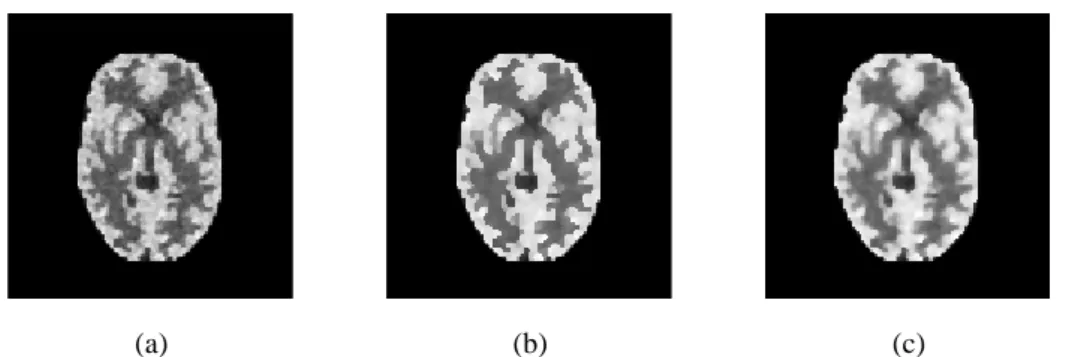
Firstly we investigate the influence of regularization parameterβ in our IIF-MAP. Reconstruction for three

different values of β with σR =0.2 and n=1 is shown in figure 3.

FIGURE 3

As is evidenced in this figure, IIF-MAP reconstruction with the bilateral filter greatly alleviates the noise artifacts in the reconstructed image. It can be seen that β controls the degree of smoothness of the

IIF-MAP reconstruction. A striking improvement can be found out that although the reconstructed images tend to be smooth, edges can be well preserved (see figure 3(b)) by choosing appropriate valueβ . This is

mainly due to the used bilateral filter which smoothes the noise while persevere salient features as well. As

the additional evidence, figure 4 shows the related line comparisons between different reconstructions

where the edge-preserving smoothing property of IIF-MAP can be readily found out.

FIGURE 4

FIGURE 5

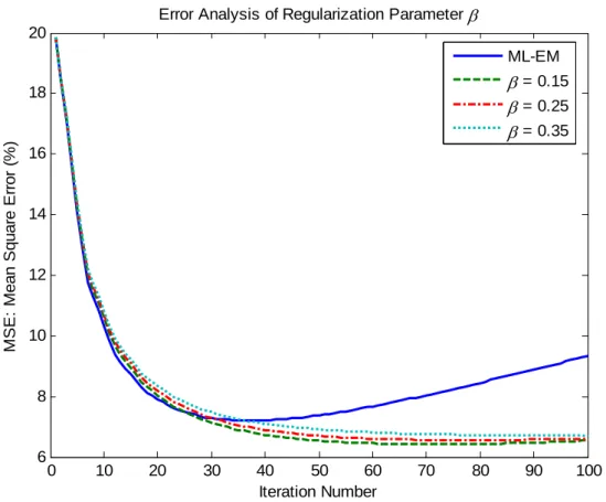
Figure 5 compares the MSE between the ML-EM and the IIF-MAP reconstructions as a function of iteration number. As noted early, the MSE in ML–EM reconstruction reaches its minimum at iteration

number 34 and then starts to increase with increasing of iteration number. However, the MSE in the

IIF-MAP algorithm continues to decrease. It also indicates from the IIF-MAP reconstructions shown in

figure 3 that the smoothing achieved by the IIF-MAP algorithm with inter-iteration filtering results in a loss

of resolution in the reconstructed images. This effect has been also observed in many other MAP image

reconstructions (e.g., [2], [3]). In fact, the IIF-MAP method can easily be reformulated as a Gaussian like

MAP estimate by choosing the priori probability density as follows:

⎥ ⎥ ⎦ ⎤ ⎢ ⎢ ⎣ ⎡ − − ∝

∑

where μ denote the mean Gaussian variables. Clearly we can set j

j k j =[H f]

μ (30)

and then readily obtain the same expression as (19).

The performance of IIF-MAP was further addressed by comparing it with TV-MAP. For each MAP

algorithm, we started with the same uniform image and then perform 100 iterations. To obtain the relatively optimal value of β for each MAP, a greedy strategy was used, which produced 100 different β values

uniformly spaced in the specific interval [0.001, 0.50]. The minimum of MSE for each β was saved

throughout the iteration progress, which is finally plotted as the function β in figure 6(a).

FIGURE 6

It is clear to see that the optimal β varies with the used MAP method. In this particular experiment,

0.006

β = yields the global MSE minimum (MSE = 6.7716) in TV-MAP while β =0.102 seems

optimal for IIF-MAP (MSE = 6.1854). Figure 6(b) shows the reconstructed images that correspond to the above two cases, i.e., β =0.006 for TV-MAP and β =0.102 for IIF-MAP. As we can see, both of

images are quite similar at least from the visual standard of view, except for the TV-MAP reconstruction

which displays several “black dots” artefact that, we believe, are caused by the numerical instability during

the calculation of the required gradient operation. Actually, one may alleviate this problem by increasing the value of ε . However we note here too large ε does change the property of TV that may result in a

totally different method. As additional evidence, figure 6(c) shows the related line comparisons between

different reconstructions of TV-MAP and IIF-MAP in which the advantage of IIF-MAP can be viewed.

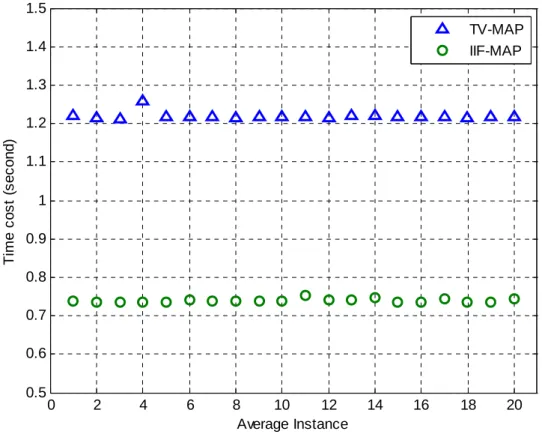
For each MAP algorithm, we also recorded the execute time calculated by averaging those CPU time costs over 100 iteration. Figure 7 shows the time cost curves generated by using TV-MAP and IIF-MAP, where

labels indicate the average cost for each 5 iteration. The total average here is 1.2202s for TV-MAP and

0.7385s for IIF-MAP respectively. It is easy to view that IIF-MAP needs few time than TV-MAP, and

nearly 40% cost is reduced. This is because the computation of bilateral filtering can be relatively more

convenient than that of TV diffusion term (27).

FIGURE 7

We shall note here that the results are provided just in our particular experimental context, which in usual

not only depend on the algorithm itself, but also can change with the programming language, code

optimization and even the configuration of the used computer. In our experiment, all of programs are coded

in C++. The computer used for simulation is with the configuration: 2.4GHz CPU and 1.0GBytes memory

storage.

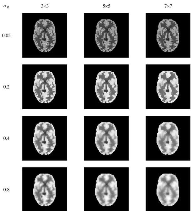
We also study the effects of parameter σ and by fixing the parameter R n β at 0.25. Reconstructions

using three different values of σ and various sizes of window are shown in figure 8. Here smooth R

images are achieved by either large or

n

n σ , as which is indicated in section 2. Similarly, smooth R

regions with sharp boundary edges can also be well preserved by relatively small value of σ . For this R

particular experiment, σR =0.2and n=1 seem to give out the best reconstruction. However, it is worthy to note that too small σ does not offer promising reconstructions as we can view from the first row of R

figure 8 (σR =0.05). In such a case, pixels with only small difference to the center one would be

overweighed so that numerous fault edges will be erroneously preserved and cause instead the noisy reconstruction. As indicated previously, given the similarity function (28) used in the bilateral filter, σ R

acts as an average edge threshold and the choice of which largely depends on the noise characteristics of measurement data. There are lots of approaches to the optimal choice ofσ . For example, one can estimate R

R

σ by either using the prior knowledge, such as the FBP reconstruction, or adaptively calculating it via the robust estimate method as it was recommended by Black et al [13]. Detailed discussion can be found in

literature [5]. We shall refer the interested reader to these literatures for more details.

FIGURE 8

3.3 Reconstruction of clinical data

This section deals with the reconstruction for the real clinical brain data. PET raw data were measured by

the currently state-of-art multi-ring PET/CT scanner (CTI Siemens Biograph Sensation 16). It can provide the highest transaxial resolution of 6.2mm FWHM and axial resolution of 4.3mm FWHM in case of

two-dimensional imaging [24]. The data acquisition commenced with the arrival of the radioactivity in the

human brain and lasted for about 30 minutes. A total number of 47 image planes were generated and the

emission data for each plane were stored in term of sinogram with size 192×192. The reconstructed images

were all set to the 128×128 pixel matrix with pixel size 2.0mm. Similarly, normalization of detector efficiencies was performed using measurements obtained from a rotating line source prior to image

reconstruction. Random coincidences were measured using the delayed time window method. The random

coincidences measured in every detector pair were subtracted from the total number of coincidences

detected by that pair.

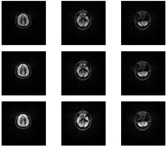
Reconstructions for several selected image planes are shown in figure 9. The reconstructions were obtained

by starting from a uniform initial image. The characteristics of the reconstructed images confirmed the

findings based on simulation studies. Images in the first row of figure 9 were obtained by running 100

iterations of the ML-EM algorithm. The ML-EM reconstruction was characteristically noisy. However, the

bias in the ML-EM reconstruction decreases with the number of iterations even though the noise is increasing. For the using of IIF-MAP algorithm, we chose to be 2 so that the resulting resolution can be

appropriate to the above given system FHWM. Images shown in the second and third row of figure 9 were n

obtained by running 100 iterations of TV-MAP and IIF-MAP respectively. Both MAP algorithms allow the

continuation of the iterations without the noise artifact but TV-MAP is slightly inferior to IIF-MAP by

producing several artefacts as demonstrated in the previous subsection. Because of the same size of used

measurement data and reconstruction, the time costs when using these MAP methods were similar to the

results as shown in the computer simulated experiments. Here TV-MAP needs 1.2326s while IIF-MAP only 0.7322s for every iteration.

FIGURE 9

In addition to these reconstructions using MAP, the regularization parameter β is chosen arbitrary since it

has proved to be difficult in clinical routine, due to the fact that a given regularization weight produces

different smoothing levels according to the patient dependent model. However, there exist a number of

methods in the literature for estimating the regularization parameter in image restoration and reconstruction problems. A number of alternative approaches for selecting regularization parameters have also been early

studied in [25], [26]. Presently, it is not clear which one of these techniques is most suitable for the present

problem of clinical PET image reconstruction. Future work is needed to study the application of these and other methods to the present problem in order to determine the optimal method for selectingβ . Finally, we

do not provide any proof of the convergence of the IIF-MAP algorithm, as this will depend on the form of the used filter and even the value of β . However, empirical evidence suggests that it usually converges

when the filter is as defined in section 2 and β is chosen properly.

4. Conclusion

To summarize, we have proposed the new method for PET image reconstruction. In this method, the

commonly used diffusion based a priori regularization is naturally approached by the new generalized inter-iteration filtering scheme. Furthermore, to overcome the filtering task but pertain to the diffusion

based MAP estimate, the extension nonlinear filter as well as the bilateral filter was employed, which

preserves the salient features of reconstructed image while smoothes away the noise. The qualitative and

quantitative evaluations of the reconstructions presented in this paper clearly indicated the feasibility and

efficiency in the reconstructed images when the IIF coupled with the bilateral filter is used.

Reference

[1] J. Llacer J and E. Veklerov, "Feasible images and practical stopping rules for iterative algorithms in

emission tomography," IEEE Trans. Med. Imag., vol. 8, pp. 186–93, 1989.

[2] T. Hebert and R. Leahy, "A generalized EM algorithm for 3-d Bayesian reconstruction from Poisson

data using Gibbs priors," IEEE Trans. Med. Imag., vol. 8, pp. 194–202, 1989.

[3] P. J. Green, "Bayesian reconstructions from emission tomography data using a modified EM

algorithm," IEEE Trans. Med. Imag., vol. 9, pp. 84–93, 1990.

[4] D. S. Lalush and B. M. W. Tsui, "A generalized Gibbs prior for maximum a posteriori reconstruction

in SPECT," Phys. Med. Biol. vol. 38 pp. 729–41, 1993.

[5] F. J. Beekman, E. T. P. Slijpen and W. J. Niessen, "Selection of task-dependent diffusion filters for the post-processing of SPECT images," Phys. Med. Biol., vol. 43, pp. 1713–1730, 1998.

[6] O. Demirkaya, "Improving SNR in PET images by using anisotropic diffusion filtration," Proceeding

of the 22nd Annual EMBS International Conference, July 23-28, Chicago IL. 2000.

[7] C. Riddell, I. Buvat, A. Savi, M. C. Gilardi, and F. Fazio, “Iterative reconstruction of SPECT data with

adaptive regularization,” IEEE Trans. Nucl. Sci., vol. 49, pp. 2350–2354, 2002.

[8] C. Riddell, H. Benali and I. Buvat, "Diffusion Regularization for Iterative Reconstruction in Emission

tomography," IEEE Trans. Nucl. Sci., vol. 51, pp. 712-718, 2004.

[9] A. B. Hamza, H. Krim and G. B. Unal, "Unifying probabilistic and variational estimation," IEEE

Signal Processing Magazine, vol. 19, pp. 37-47, 2002.

[10] P. Perona and J. Malik, "Scale-Space and Edge Detection Using Anisotropic Diffusion," IEEE Trans.

Pattern Analysis and Machine Intelligence, vol. 12, no. 7, pp. 629-639, July 1990.

[11] C. Tomasi, R. Manduchi, "Bilateral filtering for gray and color images," Proceedings of the 1998

IEEE International Conference on Computer Vision, Bombay, India, 1998.

[12] L. A. Shepp and Y. Vardi, "Maximum likelihood reconstruction for emission tomography," IEEE Trans.

Med. Imag. vol. 1, pp. 113–122, 1982.

[13] M.J. Black, G. Sapiro, D.H. Marimont, and D. Heeger, "Robust Anisotropic Diffusion," IEEE Trans.

Image Processing, vol. 7, no. 3, pp. 421-432, 1998.

[14] D. Barash, "Bilateral filtering and anisotropic diffusion: towards a unified viewpoint,"

Hewlett-Packard Laboratories Technical Report, HPL-2000-18(R.1), 2000.

[15] D. Barash, D. Comaniciu, "A common framework for nonlinear diffusion, adaptive smoothing, bilateral filtering and mean shift," Image and Vision Computing, vol. 22, pp. 73-81, 2003.

[16] N. Sochen, R. Kimmel and A.M. Bruckstein, "Diffusions and confusions in signal and image

processing," Journal of Mathematical Imaging and Vision, vol. 14, pp. 195-207, 2001.

[17] T.F. Chan, S. Osher and J. Shen, "The digital TV filter and nonlinear denoising," IEEE Trans. Imag.

Proc., vol.10, pp. 231-241, 2001.

[18] R. Kimmel, R. Malladi and N. Sochen, "Images as embedding maps and minimal surfaces: movies,

color, and volumetric medical images," Proceedings of the IEEE Computer Society Conference on

Computer Vision and Pattern Recognition, Puerto Rico, 1997.

[19] M. Elad, On the bilateral filter and ways to improve it, IEEE Trans. Imag. Proc. vol. 11, pp. 1141-1151,

2002.

[20] N. Sochen, R. Kimmel and R. Malladi, A general framework for low level vision, IEEE Trans. Imag.

Proc. vol. 7, pp. 310-318 1998.

[21] B. A. Ardekani, et al, "Minimum cross-entropy reconstruction of PET images using prior anatomical

information," Phys. Med. Biol. vol. 41, pp. 2497-2517, 1996.

[22] G. Sapiro, "Geometric Partial Differential Equations And Image Analysis," Cambridge University

Press. 2001.

[23] C. R. Vogel and M. E. Oman. "Iterative methods for total variation denoising," SIAM J. Sci. Statist.

Comput., vol. 17, pp. 227-238, 1996.

[24] G. Tarantola, F. Zito and P. Gerundini, "PET instrumentation and reconstruction algorithm in

whole-body applications," J. of Nuclear Medicine, vol. 44, pp. 756-769, 2003.

[25] A. M. Thompson, J. C. Brown, J. W. Kay and D. M. Titterington, "A study of methods of choosing the smoothing parameter in image restoration by regularization," IEEE Trans. Pattern Anal. Machine

Intell. vol. 13, pp. 326–38, 1991.

[26] R. Molina, "On the hierarchical Bayesian approach to image restoration: Applications to astronomical

images," IEEE Trans. Pattern Anal. Machine Intell. vol. 16, pp. 1122–8, 1994.

Nonlinear Filter Hk Reconstruction Filter A fk fk+1 ek k f ~ Y

Figure 1: The inter-iteration filtering scheme

(a) (b)

(c) (d) (e) Figure 2: (a) the Hoffman brain phantom, (b)-(e) ML-EM reconstructions of the simulated emission data at

iterations 10, 20, 50 and 100.

(a) (b) (c) Figure 3: Reconstructions of the brain phantom obtained by running 100 iterations of the IIF-MAP

algorithm using the bilateral filter with (a) β =0.15 (b) β =0.25 (c) β =0.35. (σ_R =0.2 and n=1

for all the case)

0 20 40 60 80 100 120 0 1 2 3 4 5 6 7 8 9 Pixel Position Pi x e l Va lu e

Error Analysis of Line Profile at Column 64

Ground truth ML-EM

β = 0.15

β = 0.25

β = 0.35

Figure 4: Comparisons of line profile at column 64 of reconstructed images.

0 10 20 30 40 50 60 70 80 90 100 6 8 10 12 14 16 18 20 Iteration Number M S E : M e an S q ua re E rro r (% )

Error Analysis of Regularization Parameter β

ML-EM

β = 0.15

β = 0.25

β = 0.35

Figure 5: The MSE between the simulated noise-free phantom image and the ML-EM and IIF-MAP (using different regularization parameterβ ) reconstructed images as a function of iteration number.

0.05 0.1 0.15 0.2 0.25 0.3 0.35 0.4 0.45 0.5 6 8 10 12 14 16 18 20 22 β T he M ini m um of M S E ( % ) TV-MAP IIF-MAP (a) (b) (c) 0 20 40 60 80 100 120 0 1 2 3 4 5 6 7 8 9 Pixel Position Pi x e l V a lu e

Error Analysis of Line Profile at Column 64 Ground truth

TV-MAP IIF-MAP

(d)

Figure 6: (a) The minimum MSE changes as a function of β where the triangles locate the global minimum MSE as well the optimal β for different MAP method; (b) and (c) are reconstructions using

TV-MAP and IIF-MAP (n=1, σ_R =0.2) respectively with optimal β indicated in (a); (d) The comparison of line profile of images shown in (b) (c).

0 2 4 6 8 10 12 14 16 18 20 0.5 0.6 0.7 0.8 0.9 1 1.1 1.2 1.3 1.4 1.5 Average Instance T im e co st ( s e c o n d ) TV-MAP IIF-MAP

Figure 7: Time cost curves generated by using TV-MAP and IIF-MAP.

R σ 3×3 5×5 7×7 0.05 0.2 0.4 0.8

Figure 8: The IIF-MAP Reconstructions with various bilateral filters. (β =0.25for all the case)

Figure 9: Reconstructions for three different slices using clinical brain PET raw data. From top to bottom: ML-EM, TV-MAP (β=0.01), and IFF-MAP (β =0.15, σ_R =0.8) respectively.