Design architecture for dynamic low inertia multi DOF robotic manipulators

(1)

1

Design Architecture for Dynamic Low Inertia Multi DOF Robotic Manipulators by

Mason Massie

Submitted to the

Department of Mechanical Engineering

in Partial Fulfillment of the Requirements for the Degree of Bachelor of Science in Mechanical Engineering

at the

Massachusetts Institute of Technology

May 2020

Signature of Author:

Department of Mechanical Engineering May 9, 2014

Certified by:

Sangbae Kim Professor of Mechanical Engineering Thesis Supervisor

Accepted by:

Maria Yang Professor of Mechanical Engineering Undergraduate Officer

(2)

2

Design Architecture for Dynamic Low Inertia Multi DOF Robotic Manipulators

by Mason Massie

Submitted to the Department of Mechanical Engineering on May 8, 2020 in Partial Fulfillment of the

Requirements for the Degree of

Bachelor of Science in Mechanical Engineering

ABSTRACT

This thesis is intended as a background for robotic designers interested in creating low inertia, high bandwidth, multi DOF robotic arms and hands capable of proprioceptive force feedback from the world.

This thesis briefly outlines the physics that govern the dynamics of robotic manipulators. It further covers various actuators and transmissions along with their dynamic and mechanical properties. Finally, this thesis covers overall robotic arm and hand architecture; where degrees of freedom can be placed and how actuators can be mounted and transmitted.

Thesis Supervisor: Sangbae Kim

(3)

3

Acknowledgements

I have many people to thank who helped get me to where I am today.

Sangbae Kim: for giving me an undergraduate research opportunity my junior and senior year while at MIT and providing me with a network of great people and tools.

Benjamin Katz: for providing constant insight and experience, help when I got stuck, and many excessively long technical conversations.

Alex Hattori: for being a great teammate on technical projects and an even better friend.

Sofia Leon: for providing valuable feedback and support.

The rest of the people in the Biomimetic Robotics Lab for inspiration and guidance.

The members of the MIT Electronic Research Society for out of the box thinking, a shared love for creating, and many fun nights.

(4)

4

Chapter 1 Introduction

1.1 Background and Motivation

The field of robotics is a rapidly growing sector. Robot usage is prevalent and expanding in manufacturing lines, warehouse distribution centers, medical surgeries and much more. As the need for robots continues to expand, humans strive to increase their capabilities. Many modern robots are capable of high speed and high precision. However, the ability to dynamically interact with the world (without breaking) and provide proprioceptive force feedback is becoming more necessary as we strive to have robots perform human like tasks. Computing power and new control strategies have enabled a vast increase in the performance of legged robots and

manipulators. However, this is only one half of the equation. Even the greatest control schemes are limited by the performance capabilities of their hardware. If we wish to continue to advance dynamic robotic capabilities, the mechanical design must be treated with as much diligence as the controls. Mechanical design is a cyclical process in which theoretical goals drive

(7)

7

development and real world constraints/ implementation details cause revaluation of the goals.

Robotic design requires a solid foundation in both the mathematical understanding of physics and the nitty gritty details. This thesis serves as a distillation of all I have learned about mechanical robotic design in pursuit of low inertia dynamic capabilities.

(8)

8

Chapter 2 Actuators

2.1 Hydraulics

Hydraulic systems use the pressurization of a liquid to create force acting upon a piston or rotary vane. Flexible hoses can be routed from ground directly to distal hydraulic actuators on a robotic arm. This can save substantial mass on the arm compared to adding a motor, especially where it matters the most towards the end effector. Hydraulics lend themselves well to high degree of freedom robot arms, as adding additional actuation is relatively easy. One central pump can create the source of power for all degrees of freedom. Hydraulic systems are capable of creating large reductions and are very resilient to impacts. Servo valves enable high frequency control of these hydraulic systems. This has been demonstrated by the dynamic capabilities of many of Boston Dynamics’ robots. Much of modern construction equipment uses hydraulic actuation as well. Hydraulics seem to fit well in the human size scale and larger. As my expertise does not lie within the design of hydraulic systems we will focus upon other systems for the rest of this paper.

2.2 Electric Motors

Electric motors are an extremely complicated and diverse topic in and of themselves. I will briefly gloss over motor basics. I encourage you to read more papers on motors and control as well as specific motor data sheets.

(9)

9

Modern electronics enable extremely high frequency control of velocity, torque, and position from electric motors. Electric motors operate very quietly while expelling no fumes or fluids making them great for indoor and near human activity. Furthermore, the energy density of modern lithium batteries has enabled mobile robots to carry their own energy sources untethered for extended periods of time. For these reasons, electric motors are extremely commonplace in the field of robotics.

Electric motors use magnetic fields to convert electrical energy into mechanical energy. Electric motors convert voltage into speed and current into force. Due to resistive losses, high currents create much more heat than high voltages do. Subsequently electric motors are great at producing small forces at high velocities.

Motors flow current through their windings to induce magnetic fields which can produce torque when interacting with other magnetic fields. Modern permanent magnets are very flux dense, subsequently most motors used in robotics elect to use permanent magnets to increase their torque density.

2.2.1 Motor Classification

Broadly speaking there are 2 fundamental types of motors, linear and rotary as can be seen below in figure 2-1 and figure 2-2.

Linear motors can only produce motion proportional to their size because they have ends. Rotary motors can produce infinite motion in a finite size because there are no rotational ends.

Figure 2-2 Rotary motor abstraction Figure 2-1 Linear motor abstraction

(10)

10

Subsequently they are prime candidates for a geared down transmission in which you trade velocity for force. The same can be done with a linear motor but the output range of motion would become extremely limited due to the reduction of the linear motor’s finite travel. For this reason, rotary motors are much more common in robotics and will be the primary focus of this section.

Within these two subsets (linear and rotary), electric motors can either have their windings mechanically commutated by brushes or electrically commutated by a controller.

Because brushless motors do not have to sacrifice space for a commutator and brushes they are more power dense than their brushed counterparts. However, they do require more advanced controllers.

In figures 2-3, 2-4, and 2-5 below black will symbolize permanent magnets and red will symbolize windings. Arrows symbolize movement of their respective colors. Generally

speaking, there are two kinds of linear electric motors: ones with stationary permanent magnets seen below in the left of figure 2-3 and ones with stationary windings seen below in the right of figure 2-3. The downside to stationary magnets is now the windings are moving and it is

subsequently harder to liquid cool them. The downside to stationary windings is that the motor is less efficient because of the windings not directly under the permanent magnets. This excess wire is not directly contributing to the force output of the motor yet it is conducting current and resulting in resistive losses.

(11)

11

Rotary motors can be subdivided again into axial flux and radial flux seen below in figures 2-4 and 2-5. The difference is how the magnets and windings are positioned to result in flux lines flowing in different directions.

(12)

12

The primary mode of heat generation in a motor is due to resistive losses in the windings. The limiting factor for steady state power and torque generation in a motor is the windings getting too hot and shorting to one another as the enamel melts. Brushless inrunners have their windings on the outside, subsequently making them easier to cool. Higher power densities can typically be achieved from brushless inrunners for this reason.

Axial Flux

Brushed Brushless Inrunner Brushless Outrunner

Figure 2-5 Axial Flux Motors: red indicates windings, black indicates permanent magnets

Radial Flux

Brushless Inrunner

Brushed Brushless Outrunner

Outrunner

Figure 2-4 Radial Flux Motors: red indicates windings, black indicates permanent magnets

(13)

13

That’s said, brushless outrunners are often favored in legged robotics because they typically have a larger air gap radius enabling them to achieve higher torque densities without the need for as large of a reduction. See “A Low Cost Modular Actuator for Dynamic Robots” for a great example.

2.2.2 Radial and Axial Flux Motor Analysis

In the field of robotics designers constantly strive to maximize the torque and power output of motors while minimizing the mass and inertia. Maximizing the torque capability 𝜏 of a motor while minimizing the rotor inertia 𝐽 enables higher peak accelerations of the motor and its load as shown by Newton’s second law. In the case of a legged robot or a vehicle, assuming the reflected rotor inertia is much less than the mass of the body, the dominant factor limiting the accelerations of the robot body becomes the motor’s torque output over the mass of the body. Often times the mass of a legged robot body can be primarily comprised of the mass of its actuators. For this reason, maximizing the torque capability of a motor while minimizing the mass 𝑚 can be beneficial for peak body accelerations. Again proven by Newton’s second law.

Seen below in figure 2-6 is a simplified diagram of an axial flux motor. 𝐷 is the diameter of the air gap of the motor while 𝑡 is the thickness of the rotor. Assume the stator has the same thickness and diameter as the rotor. Subsequently the mass of the motor will scale proportionally with the mass of the rotor, allowing us to analyze just the rotor to determine important motor trends. Assume a fixed constant 𝑐 that relates surface area at the air gap to the force produced at the rotor. This constant depends upon the field strength of the magnets, the permeability of the stator and rotor housing, the resistance and amount of windings, and the cooling rate of those windings, etc… Do not worry about the derivation of this constant, just assume 𝐹𝑜𝑟𝑐𝑒 = 𝐴_{𝑎𝑖𝑟 𝑔𝑎𝑝}∗ 𝑐.

(14)

14 𝜏 = 𝑐 ∫ 𝑟 ∗ 𝑑𝐴 (2.1) 𝜏 = 𝑐 ∫ ∫ 𝑟2 ∗ 𝑑𝑟 𝐷 2 0 ∗ 𝑑𝜃 2𝜋 0 (2.2) 𝜏 =𝑐𝜋𝐷3 12 (2.3)

Multiplying the constant 𝑐 by an infinitesimal area 𝑑𝐴 gives the force at this area. Multiplying this value again by its lever arm 𝑟 gives the torque output at this area. Now integrating this product across the entire air gap will give the total torque output of the motor seen above in equation (2.3).

𝐷

𝑡

𝑟

𝑑𝑟

𝑑𝜃

𝜃

(15)

15 𝐽 =𝑚𝑟2 2 (2.4) 𝑚 =𝜋𝑡𝜌𝐷2 4 (2.5) 𝐽 =𝜋𝑡𝜌𝐷4 32 (2.6) 𝜏 𝑚= 𝑐𝐷 3𝑡𝜌 (2.7) 𝜏 𝐽 = 8𝑐 3𝐷𝑡𝜌 (2.8)

Dividing the total torque output by the mass and inertia of the motor enables us to

analyze trends. Having a larger thickness 𝑡 enables larger magnets and more windings which can enable greater torque output. So for the sake of this analysis we will neglect this term by

assuming it would cancel out in the numerator of equations (2.7) and (2.8). Furthermore,

assuming magnetic similarity between motors, we will treat the constant 𝑐 as a constant and not a variable. Finally assuming all motors are made of similar materials, the density 𝜌 can also be treated as a constant.

This implies that increasing the diameter of the motor will enable higher torque capabilities relative to its mass. Also decreasing the diameter of the motor will enable higher torque output relative to its rotor inertia.

(16)

16 𝜏 = 𝑐 ∫ 𝑟 ∗ 𝑑𝐴 (2.9) 𝜏 = 𝑐 ∫₀2𝜋∫₀𝐿(𝐷₂)2∗ 𝑑𝑠∗ 𝑑𝜃 (2.10) 𝜏 =𝑐𝜋𝐷2𝐿 2 (2.11) 𝐽 = 𝑚𝑟2 _(2.12) 𝑚 = 𝜌𝜋𝐷𝐿𝑡 (2.13) 𝐽 =𝐿𝜋𝜌𝐷3𝑡 4 (2.14) 𝜏 𝑚= 𝑐𝐷 2𝜌𝑡 (2.15)

𝐿

𝐷

𝑑𝜃

𝜃

𝑠

𝑑𝑠

𝑡

(17)

17

𝜏 𝐽=

2𝑐

𝜌𝐷𝑡 (2.16)

We can take the exact same assumptions and analysis we used for the axial flux motor and apply it to a radial flux motor. As seen above in equations (2.15) and (2.16) we end up with the same trends in the radial case for torque over mass and torque over inertia as in the axial case. This implies that increasing the diameter of the motor will enable higher torque capabilities relative to its mass. Also decreasing the diameter of the motor will enable higher torque output relative to its rotor inertia.

2.2.3 Motor with Transmission Analysis

As mentioned before, electric motors are great at producing small forces at high

velocities relative to a human. Very rarely in robotics is a motor’s drive shaft coupled directly to a load. There is almost always a transmission of some sort which involves a reduction giving the motor mechanical advantage. To get a more holistic view of robot design we must analyze the motor in unison with the reduced transmission.

For this analysis we will neglect the mass, inertia, and inefficiencies of the transmission. We will also neglect the arm link inertia as all we care about is the actuator in this case. 𝑅 is the reduction ratio as defined below in eq (2.17). 𝐼 is the reflected inertia at the arm link which is dependent upon the product of the motor rotor inertia 𝐽 and the reduction ratio 𝑅 squared.

(18)

18 𝑅 = 𝜏𝑜 𝜏𝑚 (2.17) 𝐼 = 𝐽𝑅2 _(2.18) 𝜏𝑜= 𝜏𝑚𝑅 (2.19) 𝐼 ∝ 𝐷3𝑅2𝐿 (2.20) 𝜏𝑜 ∝ 𝐷2𝑅𝐿 (2.21) 𝑚 ∝ 𝐷𝐿 (2.22) 𝜏𝑜 𝑚 ∝ 𝐷𝑅 (2.23)

Reduction

𝑅

Motor

𝜏

_𝑚

, 𝑚, 𝐽, 𝐷, 𝐿

Arm Link

𝜏

_𝑜

(19)

19 𝜏𝑜 𝐼 ∝ 1 𝐷𝑅 (2.24) 𝑚𝐼 ∝ 𝜏𝑜2 (2.25)

(20)

20

Table 2-1 Based upon a radial flux motor with reduction as seen in figure 2-7 assume the reduction has no mass, inertia, or inefficiency.

Figure 2-11 Case 3/Case 4: pancake motor with small reduction

Figure 2-9 Case 1: constant output torque minimizing mass (high inertia)

Figure 2-10 Case 2: constant output torque minimizing reflected inertia (high mass)

Figure 2-12 Case 3/Case 4: hotdog motor with large reduction

(21)

21

As seen in table 2-7: Case 1, minimizing mass for a constant output torque can be done in two ways. The first is to increase the reduction (giving the motor more mechanical advantage) while decreasing the size of the motor correspondingly as it now needs to supply less torque. The shrinking of the motor is done by maintaining the same motor shape (a constant D/L). The second method is to increase the diameter of the motor while simultaneously making it much shorter in the axial direction. Subsequently the motor will become shaped like a pancake. The torque output of the motor is proportional to the motor diameter squared as seen in eq(2.21) yet the mass is simply proportional to the motor diameter as seen in eq(2.22). This means that as you increase the diameter; you can decrease the length by a greater amount, yielding constant torque and less mass. Both of these methods can be seen implemented above in figure 2-9.

In table 2-7: Case 2, minimizing reflected inertia while holding output torque constant can be achieved in two ways as well. The first is to decrease the reduction while increasing the size of the motor correspondingly. The enlarging of the motor is done by maintaining the same motor shape (a constant D/L). The second method is to decrease the diameter of the motor while simultaneously making it much longer in the axial direction. The torque output of the motor is proportional to the motor diameter squared as seen in eq(2.21) yet the inertia is proportional to the motor diameter cubed as seen in eq(2.20). This means that as you decrease the diameter; you can increase the length by a greater amount, yielding constant torque and less inertia. Both of these methods can be seen implemented above in figure 2-10.

In table 2-7: case 3, minimizing reflected inertia while holding output torque and motor mass constant is impossible. As seen above in eq(2.25) the torque output squared is proportional to the motor mass multiplied by the reflected inertia. This means when you hold 2 of these values constant the third is predetermined (one equation one unknown). However, the motor diameter, motor length, and reduction ratio can all be altered while still satisfying these conditions; they will just have no effect on reflected inertia. The exact same is true for case 4: holding output torque and reflected inertia constant while trying to minimize mass cannot be done.

There are many combinations of L, D, and R that can satisfy conditions for constant output torque and mass or constant output torque and reflected inertia, however they all lie upon a

(22)

22

spectrum between two extremes. The extremes are a pancake shaped motor with a small reduction, or a hotdog shaped motor with a large reduction. Both can be seen above in figure 2-11 and figure 2-12. As described in (Actuator Design for High Force Proprioceptive Control in Fast Legged Locomotion) (Seok, Wang, Otten, & Kim, 2012); in reality, gear reductions have mass, inertia, and friction. Therefore, the pancake motor with a minimal reduction is a better choice in case 3 or case 4.

(23)

23

Chapter 3 Transmissions

As stated previously, motors for robotic applications typically require reductions. As will be explored in later chapters; mounting motors far from the degrees of freedom they are actuating can be extremely beneficial for overall arm dynamics. For these reasons, transmissions are just as an important part of robotic design as the actuators. In this chapter I will outline many

transmission types and their characteristics. All transmissions are built around getting power (both force and velocity) from point a to point b.

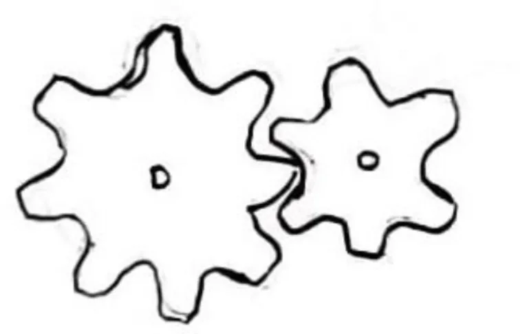
3.1 Gears

Gear transmissions are extremely commonplace in the field of robotics and for good reason. Gears rely upon the mechanical strength of their teeth pushing against one another to transmit force. The limit to the force a gear set can take is dependent upon the number of teeth in mesh and the shear strength and bending strength of those teeth. Most gears are involute,

meaning that they can be defined by three things; pressure angle, pitch, and number of teeth. The beauty of involute gears is that assuming two gears have the same tooth pitch and pressure angle

(24)

24

then they will properly mesh regardless of the number of teeth. Involute gears are conjugate curves and result in an output speed equal to the input speed.

The higher the pressure angle of a gear the stronger the tooth will be but at the expense of higher cyclical loading on each tooth and with a higher resultant separation force between the gears. Even involute gears are subject to sliding friction between the teeth. Gear sets can have efficiencies of well over 90% if designed and built properly. As the tooth pitch decreases, the amount of energy dissipated into sliding friction decreases likewise. Furthermore, for a given clearance between the center of two gears, as the tooth pitch drops, so does the backlash. Tooth strength becomes an issue when the pitch is driven too close to zero. The two most useful

equations for designing with gears are below. Metric gears have standardized pressure angles and pitch according to their module. English gears have standardized pressure angles and pitch according to their diametrical pitch.

𝑀𝑜𝑑𝑢𝑙𝑒 =𝑃𝑖𝑡𝑐ℎ 𝐷𝑖𝑎𝑚𝑡𝑒𝑟 (𝑚𝑚)

𝑁𝑢𝑚𝑏𝑒𝑟 𝑜𝑓 𝑇𝑒𝑒𝑡ℎ (3.1)

𝐷𝑖𝑎𝑚𝑒𝑡𝑟𝑖𝑐𝑎𝑙 𝑃𝑖𝑡𝑐ℎ = 𝑁𝑢𝑚𝑏𝑒𝑟 𝑜𝑓 𝑇𝑒𝑒𝑡ℎ

𝑃𝑖𝑡𝑐ℎ 𝐷𝑖𝑎𝑚𝑒𝑡𝑒𝑟 (𝑖𝑛𝑐ℎ𝑒𝑠) (3.2)

Gears come in many forms: bevel, spur, worm, helical, rack, internal, hypoid, etc… I recommend the reader look into these, however this thesis is meant as a broad background of robotic design and not a detailed explanation of gears so I will not go into details on each type. Spur gear and planetary reductions are the most common in robotics. Planetary gears can be axially cascaded to create large and compact reductions. Gears can also be used to change axis of rotation.

(25)

25

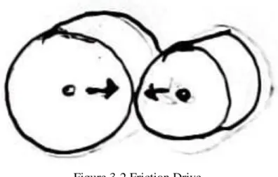
3.2 Friction Drives

Friction drives rely upon the preload between the two wheels and the coefficient of friction to transmit force. Friction drives can act as a clutch. If the torque exceeds a certain value, then the wheels will slip past each other. This can be good if a mechanical force limiter is

needed. However, after the wheels have slipped for some distance past one another, the motor encoder is no longer indicative of the output position. Therefore, either a recalibration procedure is necessary, or an encoder should be placed directly on the output.

Friction drives have inefficiencies that are a result of the two wheels deforming and undeforming as they roll with each other as a result of the normal force between them. See Hertzian contact stress for more details on this.

(26)

26

3.3 Synchronous Belts

Belts can transmit torque at distances greater than the sum of their pulley radii and come in many forms. Belts will typically have some form of flexible fiber to give them strength in tension with a rubber molded overtop. Much like a friction drive, both flat belts and V-belts rely upon the coefficient of friction between the pulley and the belt material as well as the tension of the belt to transmit torque. An advantage of both flat and V-belts is that pulleys can be made in any diameter as they are not limited by a discrete number of teeth. V-belts rely upon the angle of the V to wedge themselves into the pulley groove and attain higher friction. Unfortunately, belts that rely upon friction can slip and require either a recalibration procedure or an encoder placed directly on the output. For this reason, synchronous belts are much more common in robotics.

Synchronous belts are very lightweight and quiet. A downside to all belts is that as the belt winds and unwinds around a pulley, material is cyclically compressed and uncompressed resulting in energy dissipation through belt material damping/internal friction. Synchronous belts mitigate this issue by laying all of their fiber strands close to one another radially and designing the teeth such that they can wrap and unwrap with minimal deformation.

Synchronous belts are limited to planar actuation. Double sided synchronous belts can apply torque in both directions. For a good use of belts, see the quadruped built by Ben Katz (A Low Cost Modular Actuator for Dynamic Robots).

(27)

27

3.4 Roller Chains

Just like synchronous belts, roller chains can transmit torque at distances greater than the sum of their pulley radii. Roller chains are made from discrete pivoting links as opposed to a single piece like a belt. For this reason, chains can be easily linked and de-linked to wrap around none separating structures unlike belts. Chains are typically heavier and noisier than their belt counterparts. Chains are limited to planar actuation but can apply torque in both directions like a double sided pulley. As chain links wind and unwind around a sprocket the friction between the links and the pins resulting in energy dissipation. However, both roller chains and belts can have efficiencies above 90%. Links and pins can wear as they rub against one another creating slop that must be periodically tensioned out. For a good use of roller chains see the MIT Cheetah 3.

3.5 Linkages

Figure 3-4 Roller Chain and Sprocket

(28)

28

Linkages are simple mechanical connections that transmit force. Linkages are typically limited to planar actuation, but more complicated ones exist. For good examples of implementation look at the elbow and knee actuation of MIT Hermes and the hip abduction of the MIT Cheetah 3.

3.6 Cables/Wire Rope

Cables are extremely strong and stiff in tension for their mass. A cable is made up of many small strands of wire running parallel to one another, wound tightly in a bundle. A cable comprised of more strands per cross sectional area will be more flexible and able to bend around a tighter radius. If a single sided synchronous pulley can be thought of as a uni-directional planer device, then a double sided synchronous pulley or roller chain can be thought of as a

bi-directional planar device. In this same line of thinking a cable is essentially an infinite-directional device not limited to a single plane as seen below in figure 3-7.

Figure 3-6 Cable and Pulley

(29)

29

Cables are often given coatings to decrease sliding friction. However, when using cables on pulleys with bearings, the coatings can cause unnecessary compliance as they are tensioned around a pulley. A cable should be tensioned high enough to ensure that its natural frequency is not within the same range as the operating frequency of the joint or undesirable second order effects could be experienced in the joint. The equation governing natural frequency of a cable can be seen below in figure 3-8.

A common way of achieving high reductions and eliminating backlash with a cable transmission is by using a capstan drive. This can be done with one cable and relies upon the friction created from multiple wraps around the driving pulley. Due to the width of the cable and the diameter of the capstan, a helix angle is created. The cable terminations on the driven drum must be in line with this helix angle for the length of the cable to remain constant throughout the motion. An example of this can be seen from round to round and round to flat in figure 3-9 below. Capstan drives tend to be axially large for this reason.

If axial compactness matters, then planar drives are often used. Planar drives require 2 cables to be independently tensioned and terminated. A planar drive is limited to one half of a

Figure 3-8 natural frequency of cables

(30)

30

full rotation before the cable would try to lay overtop of itself in the same groove. A planar cable drive can be seen below in figure 3-10.

3.7 Bead Chains

Bead chains offer many of the same advantages as cables. The beads act like teeth on a cable and can transmit torque to sprockets without needing termination or multiple wraps. Bead chains act like infinite directional synchronous belts. The strength of a bead chain is limited by the central links and is typically much less than that of cables. Bead chains are common in window blinds.

Figure 3-11 Bead Chain and Sprocket

(31)

31

3.8 Flexures

Flexures are made from a single part, subsequently they are very simple and can be lightweight and inexpensive. Flexures have zero backlash and require no lubrication. Due to various manufacturing processes flexures can be made at much smaller scales than other

transmission types. Flexures have inefficiencies due to material compressing and uncompressing, resulting in energy dissipation through material damping/internal friction. The biggest handicap to flexures is their limited range of motion.

3.9 Bowden Cables

Bowden cables use a hollow outer “sheath” to guide an inner cable which can be bent in different directions. This inner cable can withstand very high forces when pulled but is subject to

Figure 3-12 Flexure

(32)

32

buckling inside of the sheath when pushed. The severity of the buckling depends upon the clearance between the cable and sheath. Bowden cables exhibit an increasing amount of sliding friction depending upon the angle to which they have been bent. They are governed by the capstan equation (3.3) seen below.

𝑇𝐿𝑜𝑎𝑑

𝑇𝐻𝑜𝑙𝑑 = 𝑒

𝜇𝜑 _(3.3)

Rather than routing a transmission through joints on a multi DOF robotic arm, Bowden cables enable actuation directly from ground to the distal joint. Bowden cables are good for actuating distal links past many degrees of freedom if force control is unimportant. Bowden cables can cause parasitic losses on a robotic arm as they require force to bend and unbend. Bowden cables can also be very useful when space does not permit room for mounting the actuator directly at the degree of freedom. Bowden cables are very commonly used to actuate bicycle brakes.

(33)

33

3.10 Flexible Shafts

Much like Bowden cables, flexible shafts enable actuation directly from ground to a distal joint. Flexible shafts can transmit torque in both directions but are subject to large amounts of sliding friction between the shaft and the “sheath”. Flexible shafts can cause parasitic losses on a robotic arm as they require force to bend and unbend. Flexible shafts are usually limited in stiffness as well. Flexible shafts can also be very useful when space does not permit room for mounting the actuator directly at the degree of freedom.

3.11 Universal Joints and Constant Velocity

Joints

Figure 3-15 Flexible Shaft

Figure 3-17 Constant Velocity Joint Figure 3-16 Universal Joint

(34)

34

Universal Joints transmit rotation from one axis to another. Universal joints have cyclical output velocity for a constant input velocity. The higher the operation angle, the less uniform the velocity becomes. However, when two universal joints are put in series and timed correctly with uniform operating angles, the final output will be a constant velocity if the input is a constant velocity. Universal joints typically cannot operate at greater than a 50-degree angle but can operate along any axis inside of that cone. Constant velocity joints are much like universal joints, except that regardless of their operating angle, they will always have the same output velocity as input velocity. Constant velocity joints are typically rated to run at less extreme angles than universal joints. Both joints are extremely common in cars as a means to transmit power from an engine to suspended wheels.

3.12 Hydraulics and Pneumatics

Pneumatics rely upon the pressurization of air, typically in a cylinder to apply force to a piston. A flexible hose can be routed from ground directly to a piston at a distal link. This can save substantial mass on a robot arm, especially where it matters the most towards the end effector. Alternatively, fluid routing can be integrated into the arm and pass through rotary links as pictured in figure 3-20. Sliding friction occurs along the seals in pistons, rotary vane actuators, and rotational links like in figures 3-18 and 3-19.

Figure 3-19 Single Vane Rotary Actuator Figure 3-18 Double Acting Cylinder

(35)

35

The pressurization of air becomes the limiting factor on how much force can be applied through a piston or rotary actuator. If the air is pressurized too high, and a tube, vessel, or piston ruptures then a violent release of energy will occur. This is equivalent to compressing a large mechanical spring and releasing it quickly. Hydraulics are much safer in this regard due to the “incompressible” nature. One advantage of pneumatics is that if a leak occurs it leaves no mess.

Hydraulics are nearly identical to pneumatics in terms of their transmissions. However, hydraulics are capable of creating much higher forces and can be controlled at a very high frequency.

Pneumatics were used to preload hydraulics through a rolling diaphragm in (A hybrid-hydrostatic transmission and human-safe haptic telepresence robot). These pistons were then coupled to a synchronous belt which drove a pulley. In this case a motor could drive one side of the system through the pulley and the second side could be coupled to an arm joint.

Both hydraulics and pneumatics are prone to inefficiency due to the viscous losses and pressure drop as fluids flow through the hosing. Pneumatic pistons are often useful for large displacements and low forces.

(36)

36

Chapter 4 Arm Architecture

4.1 Linear vs Revolute

Broadly speaking there are 2 possible robotic joints, linear and revolute. Modern bearings make achieving strong lightweight revolute designs much easier than linear/prismatic ones. This is part of the reason revolute joints are so popular in robotics. The other key to revolute joints is how distribution of mass can affect the inertial properties of the arm. In the linear case, the inertia of the moving link will be felt in its entirety when it collides with the world. Its inertia is directly proportional to its mass in this case as can be seen in the right of figure 4-1.

The case of a revolute arm is slightly different. In the worst case scenario, the mass of the moving link is entirely distributed at its distal edge. Assuming the tip of the arm collides with the world at some tangential velocity equal to the linear case, the force and reflected inertia will be exactly the same as the linear case as seen in the left of figure 4-1. In the best case scenario, the

(37)

37

mass of the moving link is entirely distributed along its axis of rotation. Assuming the tip of the arm collides with the world at some tangential velocity, the force and reflected inertia will be approximately zero as seen in the middle of figure 4-1. This is beneficial as now the moving link can dynamically collide with the world with lower forces. These attributes are particularly useful for legged robots and manipulators.

Pick and place warehouse robotics is a rapidly growing sector with commercial potential. Two degree of freedom revolute planar robot arms with an additional degree of freedom linear z axis are increasingly popular in this field. This is because they are able to reach anywhere within a cylindrical workspace while maintain a constant pitch and roll at the end effector. This helps negate the need for a “wrist” to correct orientation of the end effector as would be the case if the arm were entirely revolute joints.

Using the same inertial analysis, we will examine two possible cases of this kind of robot arm. The red represents the linear z stage and the blue represents the revolute planar arm. On the left of figure 4-2 we can see the linear stage mounted at the distal end of the planar arm. On the right of figure 4-2 we can see the linear stage mounted at the proximal end of the planar arm.

(38)

38

Placing the linear stage at the proximal end of the planar arm decreases the inertia of the arm when it moves in that plane as denoted by 𝐼𝑧𝑧 and 𝐼𝑥. However, the mass of the entire arm

will be felt as inertia at the end effector when moving vertically as denoted by 𝐼_𝑧.

Placing the linear stage at the distal end of the planar arm increases the reflected inertia at the end effector while moving in that plane as denoted by 𝐼_𝑧𝑧 and 𝐼_𝑥. However, when moving vertically now the inertia of the linear stage will be reflected at the end effector instead of the mass of the entire arm as denoted by 𝐼𝑧. This can be beneficial if the mass of your linear stage is

much less than that of the planar arm. The SCARA robot arm elected to place the linear stage at the end of the arm likely from an analysis similar to this.

4.2 Degrees of Freedom

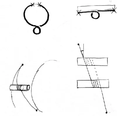
In a 3 dimensional world there are 6 degrees of freedom. A representation of this can be seen in figure 4-3. I will define position as the xyz coordinates of an object and orientation as roll pitch and yaw. For this demonstration assume serial mounting of revolute actuators. Starting with one rotational degree of freedom in figure 4-4 a position anywhere along the edge of a circle can be achieved. Each position will have a specified orientation.

Figure 4-4 One Rotational Degrees of Freedom

Figure 4-5 Two Coplanar Rotational Degrees of

Freedom

Figure 4-6 Two Orthogonal Rotational Degrees of

Freedom Figure 4-3 Six

(39)

39

Next we add a second degree of freedom in figure 4-5. Mounting another motor coplanar to this one now allows any position inside of a circle to be achieved. Again, each position will have an associated orientation. I am ignoring any duplicate orientations achieved by passing the arm through singularity. Another way to have 2 degrees of freedom is to mount a motor

orthogonal to the other as seen in figure 4-6. This case enables any point on the surface of a sphere to be reached. Again, each point will have an associated orientation.

Next we move on to a three degree of freedom system by combing the planar two degree of freedom arm with an orthogonal base motor. This can be seen below in figure 4-7. This now enables the arm to reach a point anywhere inside of a sphere. Again for each point there is an

associated orientation. This configuration is very common in robotics. It can be seen used by the Sensable Phantom and the MIT Cheetah 3.

Another possible configuration of 3 degrees of freedom is to mount them all orthogonal to each other. This can be seen in figures 4-8 and 4-9. This system allows any orientation to be achieved but with an associated position. This acts as a ball joint pictured in figure 4-10. In the three degree of freedom case pictured in figure 4-7, if the middle motor is rotated such that the distal and proximal motor are coaxial then instantaneously the system becomes two degrees of freedom. To mitigate this, the three motors should be nominally mounted orthogonal to each other as picture in figure 4-9.

Figure 4-7 Three Rotational Degrees of Freedom Pan, Tilt, and Elbow

(40)

40

Before moving on to higher degrees of freedom, I would like to display the possibility for redundancy. As seen in figures 4-11 and 4-12, motors can be mounted such that they can serve a redundant purpose. In the case of figure 4-11 the arm could move while holding a position on a plane. In the case of figure 4-12 the two coaxial motors could rotate in opposite directions to keep the exact same end point orientation but spin the arm. Redundancies typically cause excess complexity and mass and should be generally avoided. That said, a single extra redundancy in

Figure 4-8 Three Rotational Degrees of Freedom Orthogonal

Figure 4-11 Redundant Planar Arm Figure 4-12 Redundant Gimbal Figure 4-9 Three Rotational

Degrees of Freedom Gimbal

(41)

41

the arm can be valuable. Assuming the base of a robotic arm is rigidly mounted to the ground and the end effector is locked onto another rigid object, if something where to collide with the arm it would either sharply bounce off or break the arm. However, if there is a redundancy in the arm then it could move to absorb an impact while “grounded” on both ends drastically

decreasing the chances of a breakage.

Moving on from 3 degrees of freedom we see that a properly designed 6 degree of freedom arm can achieve any position with any orientation. Pictured in figures 4-13 and 4-14 it becomes clear that only one spatial spanning degree of freedom is required. We will call this degree of freedom the elbow. The shoulder and wrist need a ball joint or pan and tilt. The reason for not using more than one spatial spanning degree of freedom has to do with the inertial matrix.

If all degrees of freedom are linearly spaced along an arm, then to make small changes in orientation at the end effector will require the entire arm to move around like a snake. This will result in a very “pointy” inertial matrix. However, if 3 degrees of freedom are clustered at the wrist, then orientations changes can be made at the end effector, without input from the rest of the arm. Figure 4-13 has an advantage over figure 4-14 as its ball joint is at the base as opposed to the wrist. This means that one actuator is mounted farther away from the end effector

decreasing the inertia of the arm. Figure 4-15 demonstrates a ball joint at both the wrist and shoulder resulting in a seven degree of freedom arm. This gives the arm a single redundancy which can be helpful as discussed previously.

Figure 4-15 Seven DOF Arm, Ball Joint Shoulder and Wrist Figure 4-14 Six DOF Arm,

Ball Joint Wrist Figure 4-13 Six DOF Arm,

(42)

42

Human legs and arms are great examples of a seven degree of freedom arm. Human limbs have a ball joint at the shoulder and wrist with only one spatial spanning degree of freedom. Yaw is severely limited in the wrist and roll is severely limited in the ankle so human limbs are not dissimilar from a mixture of figure 4-13 and figure 4-15.

There is an evolutionary cost to adding more degrees of freedom to a limb. More joints mean more tendons, more muscles, and more bones. As the number of these things increases, so

does the chance that damage will occur rendering the entire limb useless. I believe nature has found the minimum number of degrees of freedom placed in series needed to achieve a good versatile performance from a limb.

(43)

43

4.3 Motor Configurations

While discussing how degrees of freedom could be placed in the previous section we assumed the output of one motor would be mounted directly to the base of the next motor and so on. This configuration is known as serial and is pictured in the left of figure 4-17. A downside to serial arms is that now the arm has a large inertia. This is because the mass of distal motors is mounted at a radius far from the base.

𝐼 = 𝑚𝑟2 _(4.1)

As seen in equation (4.1) above there are two possible ways to minimize the inertia. The first is to decrease the mass of the motors at the distal joints. This works because the torque demanded at distal joints is less than proximal joints. Distal joints have a smaller lever arm acting upon them. This method is very commonly used in industrial robot arms. Decreasing distal mass helps decrease the loads due to gravity as well. This is good because more motor torque can be allocated to performing a task as opposed to supporting the weight of the arm. The second method is to decrease the radius at which the motor mass is mounted. This can be done by moving Motor 2 along Arm link 1 to a more proximal location. A transmission is then required to pass power from Motor 2 to Arm Link 2 as their pivots are no longer coaxial. The Sensable Phantom, MIT Cheetah 3, Little HERMES 2, LIMS2-AMBIDEX, Boston

(44)

44

Dynamics Spot, and more all use this trick on 3 degree of freedom limbs to keep their motors mounted near the shoulder.

Going one step farther with the second method, Motor 2 could be mounted to the same base as Motor 1. This completely eliminates the mass of Motor 2 from affecting arm dynamics. The rotor inertia is all that will be reflected through the arm now. This configuration is called a grounded motor and can be seen in the middle of figure 4-17. Assuming a one to one reduction on the transmission, Arm Link 2 will only change its angle with respect to the ground when Motor 2 is rotated. In the serial case, Arm Link 2 will only change its angle with respect to Arm Link 1 when Motor 2 is rotated. Grounded configurations are not limited to two degrees of freedom. Look at a (6-Dof Haptic Feedback Device for Microsurgery) for inspiration.

Both motors can be grounded without the need of a conventional transmission if additional arm links are added. This configuration is considered parallel and can be seen in the right of figure 4-17. Parallel arms offer very low inertial properties enabling fast dynamics much like the grounded motor configuration. The major downside to parallel configurations is their limited workspace. This is due to the links wanting to collide with one another and more importantly singularities. Singularities are more quickly reached in parallel configurations as opposed to serial. Parallel linkages are not limited to two degrees of freedom; I have seen them go as high as six. Look at Delta style robot arms for inspiration.

4.4 Inertia vs Counterbalances

Decreasing distal mass helps decrease the loads on an arm due to gravity. However, the mass of the arm will never drop to zero. Subsequently counterbalances are often used to mitigate the loads of gravity. The downside to counterbalances is the overall increase in mass and inertia of an arm. Subsequently I will discuss the equations that govern counterbalanced arm dynamics. We will first start off by analyzing the linear case seen in figure 4-18 and move on to the

(45)

45 𝐹 = 𝑚𝑎 (4.2) 𝜏 𝑟± 𝑔(𝑚𝑐𝑏− 𝑚𝑎𝑟𝑚) = (𝑚𝑎𝑟𝑚+ 𝑚𝑐𝑏)𝑎 (4.3) 𝑎 = 𝜏 𝑟±𝑔(𝑚𝑐𝑏−𝑚𝑎𝑟𝑚) 𝑚𝑎𝑟𝑚+𝑚𝑐𝑏 (4.4)

When 𝑚_𝑎𝑟𝑚= 𝑚_𝑐𝑏, acceleration will be the same in both directions and the system will be balanced. When 𝜏 > 2𝑟𝑚𝑎𝑟𝑚𝑔 no counter balance will enable higher accelerations than an

equal weight counter balance (𝑚_𝑎𝑟𝑚 = 𝑚_𝑐𝑏).

(46)

46 𝜏 = 𝐼𝛼 (4.5) 𝜏 ± (𝑚_𝑎𝑟𝑚𝑟₂ − 𝑚_𝑐𝑏𝑟₁)𝑔 = I𝛼 (4.6) 𝐼 = 𝑚_𝑎𝑟𝑚𝑟₂2_{+ 𝑚} 𝑐𝑏𝑟12 (4.7) 𝛼 =𝜏±𝑔(𝑚𝑐𝑏𝑟1−𝑚𝑎𝑟𝑚𝑟2) 𝑚𝑎𝑟𝑚𝑟22+𝑚𝑐𝑏𝑟12 (4.8)

Assuming 𝜏, 𝑟2, 𝑟1, 𝑔 are all fixed and 𝑟1< 𝑟2. Increasing 𝑚𝑐𝑏 will increase acceleration

when spinning in the positive direction and decrease acceleration when spinning in the negative direction. When 𝑚_𝑎𝑟𝑚𝑟₂ = 𝑚_𝑐𝑏𝑟₁, acceleration will be the same in both directions and the arm will be rotationally balanced. Decreasing 𝑟₁ while increasing 𝑚_𝑐𝑏 to maintain this relation will result in higher possible accelerations by minimizing total rotational inertia. The side effect is that now the mass of the system increases. Increasing 𝑟1 while decreasing 𝑚𝑐𝑏 to maintain this

relation will result in less overall mass but at the cost of lower peak accelerations as inertia grows. Assume the motor torque is fighting the torque created by gravity on the mass on the arm.

(47)

47

Intuitively if the mass is too high relative to the torque of the motor, the inertia will dominate the acceleration. Alternatively, if the mass is too low relative to the torque of the motor, the

gravitational force will dominate the acceleration. Taking the derivative of angular acceleration with respect to the mass of the counterbalance while holding all other variables constant and setting equal to zero can yield an optimal counterbalance for acceleration. Setting an upper limit to the mass of the counter balance such that 𝑚𝑎𝑟𝑚𝑟2 ≥ 𝑚𝑐𝑏𝑟1 is reasonable.

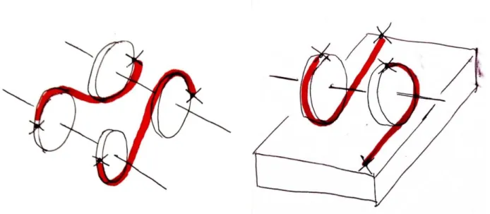
4.5 Decoupling

When grounding a motor and wishing to actuate far distal joints the transmission must be routed through all intermediate links. If the movement of an intermediate joint affects the motion of a distal join, then those joints are said to be coupled. Often times the motors used for gripping

objects at an end effector are designed for lower force and reflected inertia. More proximal motors are often larger to support greater loads and subsequently maintain higher rotor inertia. Coupling can be bad because as high fidelity operations are performed with the end effector, if

𝟒

𝟒 +

𝟒

𝟒 = 𝟐

𝟑

𝟒 +

𝟓

𝟒 = 𝟐

Figure 4-20 Revolute Joint with Planar 3 Pulley Cable Transmission

𝟏

𝟐 +

𝟏

𝟐 = 𝟏

𝟎

𝟐 +

𝟐

𝟐 = 𝟏

Figure 4-21 Revolute Joint with 2 Belts and Idler Pulley

(48)

48

the arm moves simultaneously, then the force, and reflected inertia of proximal motors can be felt at the end effector.

In figure 4-20 as denoted by the equations, an idler pulley with two belts on a revolute joint has no total change in belt length as the black number remains constant. However there is coupling as shown by the change in blue and red numbers. In figure 4-21 as denoted by the equations, a planar cable drive with 3 sets of pulleyshas no total length change but is coupled.

However a “double jointed” arm maintaining a roll without slip condition has zero coupling as cables are passed through it. It also has zero total length change in the cables. This joint can be seen in figure 4-22.

This kind of analysis can be used on any set of pulleys/ sprockets to determin coupling.

4.6 Range of Motion and Self Intersection

Simple revolute joints have the issue that when arm link 2 is rotated with respect to arm link 1, they will want to intersect. If rotations greater than plus or minus 90 degrees wish to be

𝟐

𝟒 +

𝟐

𝟒 = 𝟏

𝟐

𝟒 +

𝟐

𝟒 = 𝟏

(49)

49

achieved, large sections of the arms must be cut out to avoid intersection. This results in poor torsional and bending stiffness.

1 way to avoid self-intersection at angles close to 180 degrees is to put a bend in the arm as seen below in figure 4-24. This enables 180-degree operation on one side but it cannot go much past 0 degrees in the opposite direction.

Figure 4-23 Revolute joint clearance to avoid self-intersection

(50)

50

Simple revolute joints have the issue that when arm link 2 is rotated with respect to arm link 1, they will want to intersect. A simple way to avoid this is to offset the plane of Arm link 1 relative to Arm link 2. This enables full 360-degree rotation which is good. An example can be seen in figure 4-25 below. The downside is now your shaft is in single shear as opposed to double shear which is bad for stiffness and strength.

“Double” joints that maintain a roll without slip condition are able to rotate plus or minus 180 degrees with zero self-intersection. This is actually very similar to how human elbow and knee joints work. Two bones roll against one another and ligaments hold them together. The downside is that these kinds of joints are more complex and difficult to actuate.

Figure 4-25 Single Shear Offset Revolute Joint with “Grounded” Motors

(51)

51

4.7 Locations of Reductions

𝜏𝑜 𝜏𝑚= 𝑅 (4.9) 𝜏𝑚 𝑟 = 𝑇1 (4.10) 𝜏𝑜 𝑟 = 𝑇2 = 𝑅𝜏𝑚 𝑟 (4.11)

In the case of the reduction being at the joint, the tension force applied to the belt is lower by a factor of R than when the reduction is at the motor. By decreasing the force on transmission components, they can be made lighter and smaller decreasing the inertia of a limb. However, reductions typically have some associated mass. By moving this mass farther away from the center of rotation, reflected inertia can be increased. Locating the reduction at the joint must be decided upon in a case by case basis as it depends heavily upon details of mechanical

implementation.

(52)

52

Chapter 5 Hand Architecture

5.1 Human Hand

When many people think of a general purpose robot hand, they want to start with the human hand as a major point of reference. Human muscle is very different from electric motors. Subsequently design of a robotic hand should be thought about from the ground up on how to take advantage of electric motor design characteristics.

Human muscle is very force dense with low inertia. Muscles can be scaled to any size by changing the amount of muscle fibers in a strand. For this reason, there is a very low cost to adding small additional degrees of freedom in a hand. Unfortunately, electric motors do not operate at small scales as nicely as muscle fibers. Human hands have 27 degrees of freedom, trying to design a similar robotic hand results in something excessively complex and fragile. Furthermore, a large bulky mass of 27 actuators is typically housed in what would be considered the forearm, decreasing the dynamic capabilities of the arm as a whole.

Muscles can only pull in tension and subsequently come in antagonistic pairs. Electric motors can apply torque on both directions and are not limited to the same rules as muscles. To design an effective robotic hand, we must start from scratch without any prior conceptions of what a hand “should” look like.

5.2 Constraining Degrees of Freedom

A good starting point for hand design is to determine how many ways objects can be constrained by a grip with the simplest “fingers” possible. This is outlined below in figure 5-1.

(53)

53

5.3 Minimum Viable Hand

A good approach to hand design is to determine the fewest degrees of freedom necessary to accomplished desired tasks. Then to implement those degrees of freedom in a lightweight and simple manner.

At some point, for manipulation, having a second simple hand becomes much more valuable than having a more complex hand. Just try tying your shoes with one human hand, you will find it extremely difficult even with all 27 degrees of freedom. Now try it with only the index finger and thumb of your two hands. Much easier.

The da Vinci surgical robot is able to do very complex surgery by having two hands with one simple pinching degree of freedom each. The wrists of the robots have 3 degrees of freedom which enables reorientations of the end effector without moving the entire arm.

(54)

54

A single degree of freedom past the wrist is surprisingly capable. Moving forward from one degree of freedom each additional degree of freedom provides additional value but at a diminishing rate. I feel as though four degrees of freedom is the next substantial step up in capabilities. As can be seen in figure 5-2 squeeze grasp, retention grasp, point grasp, and ledge grasp are all capable from a hand with 4 degrees of freedom. This is done by rotating 2 of the fingers at their base to reconfigure the shape of the hand. The Barrett hand is a prime example of the capabilities a four degree of freedom hand can offer.

As a hand progresses past 4 degrees of freedom, each finger can be thought of as an individual arm. Giving each finger the capability of reaching a point inside of a spherical workspace allows them to act as individual limbs on top of the palm. This requires 3 degrees of

(55)

55

freedom per finger. Multiplying this by three fingers results in nine total rotational degrees of freedom for the hand. Ishikawa Komuro Lab's high-speed robot hand is a great example of the multifaceted capabilities a hand of this many degrees of freedom can possess. The base of one finger was mounted directly to the palm eliminating one degree of freedom in this case leaving eight total.

The issue with 8 degrees of freedom in a hand is that all of the mass of the motors for the fingers is located at the tip of the arm. Pushing the finger and wrist motors back to a more proximal location near a shoulder would solve this issue. However, it can become exceedingly complex to try to route a transmission through a 3 degree of freedom wrist and an elbow. For this reason, I have come to the conclusion that if you wish the mount electric motors at a shoulder that actuate a small distal hand; a simple one degree of freedom gripper is all that can be feasibly accomplished. See the da Vinci Surgical robot for a great implementation of this. If a high degree of freedom hand is necessary, the alternative is to decrease the mass of the finger motors and directly mount them at the hand.

Figure 5-3 through figure 5-7 below show a two degree of freedom wrist with a one degree of freedom parallel pincher all actuated by motors mounted at the shoulder via a cable transmission. I designed the wrist and gripper to mount directly onto Benjamin Katz’s three degree of freedom arm. This hand was designed for bilateral teleoperation. As you can see, very large motors were used for the wrist and pincher relative to the size of the hand enabling high output torque. Yet the reflected inertia of the gripper and entire arm were kept extremely low by locating the motors at the base of the arm and using minimal reductions.

(56)

56

Figure 5-4 Five DOF Cable Driven Robotic Arm with One DOF Gripper

Figure 5-4 Two DOF Cable Driven Robotic Wrist with One DOF Gripper

(57)

57

(58)

58

Figure 5-6 Cable Routing through Wrist and Elbow Idler

Figure 5-7 Motor Gear Reduction and Cable Routing to Motor Pulleys

(59)

59

Chapter 6 Summary and Conclusion

Mechanical robotic design is a cyclical process in which theoretical goals drive

development and real world constraints/ implementation details cause revaluation of the goals. Design requires a solid foundation in both the mathematical understanding of physics and the nitty gritty details. This thesis outlined the physics that govern the dynamic capabilities of electric robotic actuators. It further provided a brief overview of prevalent transmissions in robotics and their associated implementation details. Finally, high level architecture of robotic arm and hand design was explored in terms of governing physics and real world limitations. This thesis serves to inform design strategies in pursuit of furthering the dynamic and proprioceptive capabilities of robotics.

(60)

60

Bibliography

[1] Seok, S., Wang, A., Otten, D., & Kim, S. (2012). Actuator design for high force

proprioceptive control in fast legged locomotion. 2012 IEEE/RSJ International Conference

on Intelligent Robots and Systems. doi:10.1109/iros.2012.6386252

[2] P. M. Wensing, A. Wang, S. Seok, D. Otten, J. Lang and S. Kim, "Proprioceptive Actuator Design in the MIT Cheetah: Impact Mitigation and High-Bandwidth Physical Interaction for Dynamic Legged Robots," in IEEE Transactions on Robotics, vol. 33, no. 3, pp. 509-522, June 2017, doi: 10.1109/TRO.2016.2640183.

[3] Kim, Y. (2015). Design of low inertia manipulator with high stiffness and strength using tension amplifying mechanisms. 2015 IEEE/RSJ International Conference on Intelligent

Robots and Systems (IROS). doi:10.1109/iros.2015.7354208

[4] Katz, B. (2018). A low cost modular actuator for dynamic robots.

[5] https://web.stanford.edu/group/sailsbury_robotx/cgi-bin/salisbury_lab/?page_id=399 [6] http://ishikawa-vision.org/facility/index-e.html [7] https://advanced.barrett.com/barretthand [8] https://www.davincisurgery.com/da-vinci-systems/about-da-vinci-systems [9] https://www.bostondynamics.com/ [10] https://www.youtube.com/watch?v=97KX-j8Onu0 [11] https://techtv.mit.edu/videos/467-robotic-gripper-with-phantom-sensable-technologies