HAL Id: hal-00298708
https://hal.archives-ouvertes.fr/hal-00298708
Submitted on 8 Sep 2005HAL is a multi-disciplinary open access
archive for the deposit and dissemination of sci-entific research documents, whether they are pub-lished or not. The documents may come from teaching and research institutions in France or abroad, or from public or private research centers.
L’archive ouverte pluridisciplinaire HAL, est destinée au dépôt et à la diffusion de documents scientifiques de niveau recherche, publiés ou non, émanant des établissements d’enseignement et de recherche français ou étrangers, des laboratoires publics ou privés.
Distance in spatial interpolation of daily rain gauge data
B. Ahrens
To cite this version:
B. Ahrens. Distance in spatial interpolation of daily rain gauge data. Hydrology and Earth System Sciences Discussions, European Geosciences Union, 2005, 2 (5), pp.1893-1922. �hal-00298708�
HESSD
2, 1893–1923, 2005Distance in spatial interpolation of daily
rain gauge data
B. Ahrens Title Page Abstract Introduction Conclusions References Tables Figures J I J I Back Close Full Screen / Esc
Print Version Interactive Discussion
EGU
Hydrol. Earth Sys. Sci. Discuss., 2, 1893–1923, 2005 www.copernicus.org/EGU/hess/hessd/2/1893/
SRef-ID: 1812-2116/hessd/2005-2-1893 European Geosciences Union
Hydrology and Earth System Sciences Discussions
Papers published in Hydrology and Earth System Sciences Discussions are under open-access review for the journal Hydrology and Earth System Sciences
Distance in spatial interpolation of daily
rain gauge data
B. Ahrens
Institut f ¨ur Meteorologie und Geophysik, Universit ¨at Wien, Austria
Received: 10 August 2005 – Accepted: 29 August 2005 – Published: 8 September 2005 Correspondence to: B. Ahrens ([email protected])
HESSD
2, 1893–1923, 2005Distance in spatial interpolation of daily
rain gauge data
B. Ahrens Title Page Abstract Introduction Conclusions References Tables Figures J I J I Back Close Full Screen / Esc
Print Version Interactive Discussion
EGU
Abstract
Spatial interpolation of rain gauge data is important in forcing of hydrological simula-tions or evaluation of weather predicsimula-tions, for example. The spatial density of available data sites is often changing with time. This paper investigates the application of sta-tistical distance, like one minus common variance of time series, between data sites
5
instead of geographical distance in interpolation. Here, as a typical representative of in-terpolation methods the inverse distance weighting inin-terpolation is applied and the test data is daily precipitation observed in Austria. Choosing statistical distance instead of geographical distance in interpolation of an actually available coarse observation net-work yields more robust interpolation results at sites of a denser netnet-work with actually
10
lacking observations. The performance enhancement is in or close to mountainous terrain. This has the potential to parsimoniously densify the currently available obser-vation network. Additionally, the success further motivates search for conceptual rain-orography interaction models as components of spatial rain interpolation algorithms in mountainous terrain.
15
1. Introduction
Precipitation maps with daily or better resolution are necessary for investigation of the climatology of extreme events (e.g.Skoda et al.,2003;Palecki et al.,2005), as input in hydrological modeling (e.g.Singh and Frevert,2002a,b), or in evaluation of numerical weather prediction models (e.g.Beck and Ahrens,2005), for example. Depending on
20
application the maps have to be available close to real-time (e.g. in detection of flood generating processes) or it is possible to wait some time and gather as much rain observation data as possible (e.g. in climatology).
The back-bone of these maps are rain gauge data since the reliability of remote sensing data (e.g. by weather radar or satellite) is not high enough (e.g.Young et al.,
25
tempo-HESSD
2, 1893–1923, 2005Distance in spatial interpolation of daily
rain gauge data
B. Ahrens Title Page Abstract Introduction Conclusions References Tables Figures J I J I Back Close Full Screen / Esc
Print Version Interactive Discussion
EGU
ral variation of spatial coverage of available rain gauges. For example, the monthly monitoring product of the Global Precipitation Climatology Centre (http://gpcc.dwd.de) is based on about 6000 stations available in near real-time. A second product, the so-called full product, is based on 40 000 stations in the late 1980s but based on only about 20 000 stations in the year 2000. Another example of time-delay in data
avail-5
ability is a daily precipitation atlas by Rubel(1996) with gridspacing of a few tens of kilometers for the Baltic sea and its drainage basin (area: 1.7e6 km2). Rubel(1996) is based on about 400 stations and its update byRubel and Hantel(2001) is based on a 10-times denser station network.
Auer et al. (2005) developed a homogenized dataset of long series of monthly
pre-10
cipitation at 192 station sites in the European Alps and their surroundings. But the average site-to-site distance increases backwards in time from 61 km in the second half of the 20th century to 74 km in the late 19th century and up to about 200 km in the early 19th century. Relative series homogenization relies on significant common variability between neighbored site series assumed to be expressible as common
vari-15
ance R2with R the linear correlation coefficient. Auer et al.(2005) chose a threshold of R2=0.5 and thus relative homogenization is not possible in the early 19th century followingScheifinger et al.(2003) who estimated a network density of about 1/100 km to have the necessary common variance in the greater Alpine region.
For daily precipitation Scheifinger et al.(2003) recommended an average distance
20
of 40 km or better in relative series homogenization. Therefore, likewise dense obser-vation networks for mapping of daily data are wished, but, of course, are not available in most regions at most times. Nevertheless, mapping is done since (a) a low-quality map is better than nothing and (b) the necessary station density is reduced by smooth-ing: mapping or regionalization is interpolation of point data (the rain gauge orifices of
25
∼1000 cm2 are small compared to the mapping scale, thus the observation sites are considered to be points in good approximation) and spatial averaging or smoothing of the interpolated point data. This leads to precipitation fields with spatial gridspacing and cell support of, for example, a few tens of kilometers.
HESSD
2, 1893–1923, 2005Distance in spatial interpolation of daily
rain gauge data
B. Ahrens Title Page Abstract Introduction Conclusions References Tables Figures J I J I Back Close Full Screen / Esc
Print Version Interactive Discussion
EGU
This paper discusses the point data interpolation part of mapping only. The separate problem of support change by averaging is not discussed. Another challenge not to be discussed here is the correction of rain gauge data for systematic errors which can be due to wind-induced or evaporation loss (Rubel and Hantel,1999).
For illustrational purposes we apply the Inverse Distance Weighting interpolation
5
(IDW) method. IDW assigns weights to neighboring observed values based on distance to the interpolation location and the interpolated value is the weighted average of the observations. IDW is applied in many precipitation mapping methods (e.g.Rudolf and
Rubel,2005;Frei and Sch ¨ar,1998) often enhanced with add-ons like declustering and directional grouping of stations, or empirical adjustments in respect to orography (Daly
10
et al.,1994). The IDW method is an example of a deterministic interpolation method. Statistical interpolation methods like Kriging are optimal in a statistical sense, but not robust in data sparse regions. A successful application of a statistical interpolation method is presented inRubel and Hantel(2001).
The IDW method is an implementation of Tobler’s first law of geography (Tobler,
15
1970): all things are related, but nearby things are more related than distant things. Generally, in spatial interpolation the distance is measured by the geographic distance. The idea of this paper is to use the statistical distance between precipitation time series at the interpolation site and actually available observation sites as distance measure in the IDW method. It shall be shown that this is a parsimonious and robust method
20
to in-fill a coarse network of actually available observations by using information of a denser network that is not available for the interesting time period.
2. Data
For evaluation of precipitation interpolation methods assuming different mean observ-ing station distances a dense reference network of precipitation stations is necessary.
25
In this investigation a data set of about 900 stations with long daily time series (in the period 1971 to 2002) has been available for Austria (total area is 84 000 km2) as
pro-HESSD
2, 1893–1923, 2005Distance in spatial interpolation of daily
rain gauge data
B. Ahrens Title Page Abstract Introduction Conclusions References Tables Figures J I J I Back Close Full Screen / Esc
Print Version Interactive Discussion
EGU
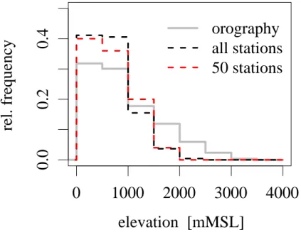
vided by the Hydrographisches Zentralb ¨uro, Vienna (delivery date: February 2005). Austria is a country in Central Europe with 62% covered by the Austrian Alps and only 32% below 500 m, cf. Fig. 1, and thus interpolation is done in complex mountainous terrain.
The chosen year for the interpolation experiments is 1999. All stations with missing
5
data in 1999 and not at least twenty years of data are erased from the data set and the investigations are done with the remaining 710 station time series. This set of stations is named ALL in the following.
In the set ALL the mean next station inter-distance is 6.7 km, but the stations are not regularly distributed within the domain of investigation, i.e. Austria. They are clustered
10
around Vienna in the north-east of the domain and in the main Alpine valley floors (Fig. 2). The irregularity is also illustrated in Fig. 1 which compares the orographic height distribution with distributions of station heights. The lower altitudes are relatively better represented by stations than higher elevations.
In the interpolation experiments we applied subsets of ALL stations with 25, 50, and
15
150 members as observing stations and subsets of the remaining stations with 300 members as evaluating stations. We draw the subsets in a fashion that approximately maximizes the next station geographic inter-distance. One station of the minimum distance pair is erased until the wished number of observing and subsequently of eval-uating stations is left. Table1 gives minimum, mean, and maximum geographic
dis-20
tance and next neighbor common variance R2. The mean R2 increases with number of stations as expected and consequently the mean interpolation performance should increase. It is noteworthy that for all station sets there are sites which are statistically far from all the others, i.e. R2<0.5.
The chosen regularizing sub-sampling leads to declustering of the considered station
25
sets, but as Fig. 1 illustrates the elevation distribution of the stations is only slightly improved. It should be kept in mind that typical station networks are clustered and thus the effective number of stations in mapping is smaller than the nominal number of stations. We did experiments with random sub-sampling which lead to decreasing
HESSD
2, 1893–1923, 2005Distance in spatial interpolation of daily
rain gauge data
B. Ahrens Title Page Abstract Introduction Conclusions References Tables Figures J I J I Back Close Full Screen / Esc
Print Version Interactive Discussion
EGU
interpolation performance, but this will not be discussed further.
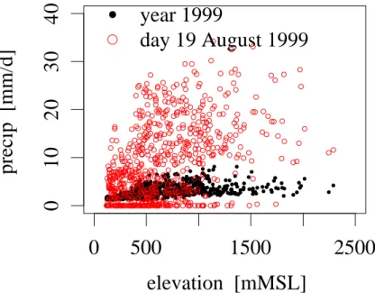
In climatological mapping of precipitation in mountainous terrain a precipitation-elevation relationship is often successfully considered (cf. Sevruk, 1997). This ele-vation dependence is illustrated in Fig.3for yearly data. It is also illustrated that such a dependence is less obvious at shorter time scales because of the large scatter of the
5
daily precipitation values. This will be discussed in some more detail in the following section.
3. Interpolation method
The Inverse power of Distance Weighted interpolation (IDW) is applied. In standard IDW the interpolated value is estimated by a weighted mean of the observations and
10
the weights are proportional to a negative power of geographical distances dα be-tween the point of interpolation and the considered observation points. Typically, not all observations Pαare considered in estimation of the interpolating value P0but only n neighboring with P0= Pn α=1Pαwα Pn α=1wα (1) 15
and the weights wα = 1
dαλ
(2)
The power λ of distance has to be chosen appropriately depending on the interpolated variable. Spatially smoother variables show larger spatial dependence and thus like smaller values of λ than spatially rougher fields. Generally, it is assumed that the
20
separation of close-by observations increases faster than linear with station distance and often a power λ of two is assumed.
HESSD
2, 1893–1923, 2005Distance in spatial interpolation of daily
rain gauge data
B. Ahrens Title Page Abstract Introduction Conclusions References Tables Figures J I J I Back Close Full Screen / Esc
Print Version Interactive Discussion
EGU
If only the next neighbor is considered (i.e. n=1) IDW collapses to the next neighbor or Thiessen method. AsBl ¨oschl and Grayson(2001) elaborated, IDW generates spu-rious artefacts in case of highly variable quantities and irregularly spaced data sites. This is typical for observed precipitation data. Thus, in practical implementations the IDW is complemented by empirical methods like directional grouping of stations and
5
exclusion of stations if shadowed by closer stations (Shepard,1984). These artefacts are not important in our experiments because of the applied regularizing sub-sampling of the available stations. IDW interpolation applying geographical distance is named d -IDW in the following.
Besides geographical distance additional empirical relationships can be
imple-10
mented. One example is regression with orography (Daly et al.,1994). Adopting this regression is crucial in development of climatological precipitation maps but of less im-portance in daily maps as Fig.3 indicates. But this example illustrates that besides horizontal distance also vertical distance, slope of orography, observation positioning at the wind- or leeward slope, distance from the range crests etc. should be considered
15
(Smith,1979). Unfortunately, implementations of adequate empirical relations of that type are difficult (Smith,2003;Barros and Lettenmaier,1994). A simple station sep-aration measure is wanted which takes the complexity of rain-terrain interaction into account.
Here, we assume that long time series of precipitation are available at the
observa-20
tion sites and the interpolation sites. Thus, it is easy to replace geographical distance by some type of statistical distance between data series. A proper statistical station distance implicitly considers rain-terrain interaction through experience. One useful class of statistical measures obviously are cross-correlation type measures like 1−R2. The drawback of this measure of proximity is that differences in the mean between
25
neighboring series are not considered. Therefore, we apply as an alternative statistical measure of separation the semi-mean squared difference (i.e. basically the Euclidian
HESSD
2, 1893–1923, 2005Distance in spatial interpolation of daily
rain gauge data
B. Ahrens Title Page Abstract Introduction Conclusions References Tables Figures J I J I Back Close Full Screen / Esc
Print Version Interactive Discussion EGU distance) γ0α = 1 2T T X t=1 (Pt0− Ptα)2 (3)
between the time series of length T . Only days t with precipitation at both observa-tion sites 0 and α are considered. This measure quantifies random and systematic differences between the time series.
5
If γ is applied in IDW the proximity of stations is replaced with the proximity of data series. The resulting interpolation method is named γ-IDW in the following.
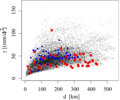
Application of d - or γ-IDW yields different interpolation values since geographical close-by stations can observe relatively distant precipitation time series and vice versa. This is shown in Fig.4. Tobler’s law is valid in a mean sense, but for single evaluating
10
stations the next geographical neighbor might not be the next neighbor measured by the γ-distance (exemplified by two station’s γ-vectors marked red and blue in the fig-ure). Therefore, application of the γs instead of the d s changes the selection of the n next neighbors and their relative importance in the interpolated value.
The factor 1/2 in the definition of γ is not important here, but chosen to illuminate
15
that the scattergram shown in Fig.4would be the empirical semi-variogram in case of Kriging with a climatological semi-variogram like inRubel and Hantel(2001). Addition-ally, it shall be mentioned that it is equally easy to apply a Kriging variant instead of IDW for the interpolation experiments discussed here.
Figure5indicates the spatial and statistical representativeness of the observing
sta-20
tions of set 50. Shown are the averaged inverse distances to the neighboring 24 eval-uating station sites (i.e. about to neighbored evaleval-uating sites to which the observing stations are applied to in interpolation with n=4). The geographical representativeness of the stations scatter but is not systematically dependent on station elevation. This confirms that the regularizing sub-setting has been successful. The statistical
repre-25
sentativeness decreases with station elevation on average. Since this is not respected by geographical distance weighting and since mean observed precipitation increases
HESSD
2, 1893–1923, 2005Distance in spatial interpolation of daily
rain gauge data
B. Ahrens Title Page Abstract Introduction Conclusions References Tables Figures J I J I Back Close Full Screen / Esc
Print Version Interactive Discussion
EGU
with height it is expected that precipitation will be tendencially overestimated in the Alpine area by interpolation with d -IDW. Additionally, n might be chosen larger or the exponents λ chosen smaller in the eastern lowlands of Austria than in the Alpine area in an optimized d -IDW interpolation setup to compensate the varying data representa-tiveness (not tested here).
5
As mentioned above the γs also measure systematic differences in time series which may be due to elevation dependence of precipitation in orography, mountain shadowing effects, or horizontal trends in the precipitation field, for example. These systematic differences are not measured by the centered semi-mean squared difference
γ0α0 = 1 2T T X t=1 ((Pt0− m0) − (Ptα− mα))2 (4) 10
with m the time series means.
The effects of systematic differences on statistical distances are shown in Fig. 6. The relative effect (γ0−γ)/γ over geographical distance is given for four classes of station elevation differences. For geographically nearby stations the importance of systematic differences is increasing with station elevation difference. On average the
15
effect of systematic difference between nearby stations with almost no vertical elevation difference is below 1%. This effect is about 7% for stations with about 1000 m vertical distance. This is consistent with Haiden and Stadlbacher(2002). They found for the same data an elevation dependence of yearly precipitation amounts up to 20% per 1000 m height difference if they restricted their evaluation to station pairs with horizontal
20
distances smaller than ten kilometers.
With increasing horizontal distance the height difference gets less important. For d≤100 km trends due to shadowing effects in complex terrain might be important and the remaining height correlation shown in Fig.6might be due to a shadowing proba-bility that is increasing with larger station height differences. For even larger horizontal
25
distances a pronounced east-west gradient in Austrian precipitation sums (cf. Fig. 8) might explain the increasing differences between γ and γ0. The vertical difference
de-HESSD
2, 1893–1923, 2005Distance in spatial interpolation of daily
rain gauge data
B. Ahrens Title Page Abstract Introduction Conclusions References Tables Figures J I J I Back Close Full Screen / Esc
Print Version Interactive Discussion
EGU
pendence is probably artificial since the relative frequency of orographic heights differs substantially between eastern and western Austria. Here, we present possible reasons of systematic effects only without further discussion, but their existence motivates the usage of γ instead of γ0or R2as the statistical distance measure. In either interpolation method these trends have to be considered adequately.
5
The γ-IDW can be applied only at interpolation sites with long time series of pre-cipitation observations. At non-observation sites a mixed method could be thought of. The n next neighbors are determined by geographical distance. For the neighbors long precipitation time series are available and thus their d and γ inter-distances can be determined. With this information a simple approximation for statistical distances of
10
the interpolation site to the next neighbors can be derived. Geometrical selection com-bined with approximated statistical distances and thus approximated statistical weights generates an interpolation method that is slightly better than d -IDW but shall not be further discussed here. The performance gain is small indicating that orogenic modifi-cations on statistical distance are non-homogeneous and anisotropic in space.
15
4. Results
As already noted the interpolation experiments are done with the observing station data sets of size 25, 50, and 150 for the year 1999. Always 300 evaluating station sites are the considered interpolation points and thus evaluating data is available. Figure7
compares the results of d - and γ-IDW interpolation. In this example the number of
20
observing stations is 50 and next-neighbor interpolation, i.e. n = 1, is applied. It is shown that often the next neighbor and thus the interpolation value differ between the two approaches. In next-neighbor γ-IDW interpolation even two stations (Mitterfeldalm (1665 m MSL) and Filzmoos (1060 m MSL) circled in Fig.7) are not considered in inter-polation. The spatial representativeness of these stations is relatively small and thus
25
the observations at these stations are statistically useless for next-neighbor interpola-tion.
HESSD
2, 1893–1923, 2005Distance in spatial interpolation of daily
rain gauge data
B. Ahrens Title Page Abstract Introduction Conclusions References Tables Figures J I J I Back Close Full Screen / Esc
Print Version Interactive Discussion
EGU
The interpolation results are compared to the evaluating observations with simple statistics like relative bias B=(mean(I)−mean(O))/mean(O) with I a set of interpolated values and O the corresponding set of evaluating observations at the interpolation sites, linear correlation R(I, O), the ratio of standard deviations σ(I)/σ(O), and e ffi-ciency E=1−mean((I−O)2)/σ2(O)=1−MSE(I, O)/σ2(O). The spatial average of time
5
series biases is denoted by Bt.and the temporal average of biases between daily pre-cipitation fields is denoted B.s. The dot indicates the finally averaged dimension. The same notation is applied to the averaged correlations, standard deviations and e fficien-cies. In case of a perfect interpolation the values of the bias statistics are identical zero and the other statistics’ values are one.
10
Table2shows mean results of the evaluation. As expected the correlation of inter-polated values with evaluating data increases with the number of observing stations. Improvement of bias is not that obvious. Changes in the exponent λ have a smaller impact, but are not unimportant. The evaluation indicates that in d -IDW an exponent smaller than two performs best in the yearly average. More important is the number
15
n of considered observation neighbors. In case of 50 observing stations four-neighbor interpolation is better than next-neighbor interpolation but there is no relevant improve-ment in taking eight neighbors and even slight decrease in interpolation performance if sixteen neighbors are taken. A similar number of neighbors are optimal in case of 25 or 150 observing stations.
20
The γ-IDW interpolation is better in correlation and efficiency but seems to be worse in bias. In d -interpolation there is a more pronounced spatial compensation of er-rors. Underestimation, for example close to the southern Austrian border (cf. Fig.8), is compensated by a tendency for overestimation in central Alpine areas by geograph-ical interpolation. This is due to overestimation of representativeness of high-elevation
25
observations (cf. Fig.5). The tendency for underestimation in γ-interpolation can be avoided if the statistical distances are estimated after logarithmic transformation of the time series (cf. experiment ln in Table2). This effectively reduces the positive skewness of the intensity distribution of daily precipitation. The skewness of the precipitation
dis-HESSD
2, 1893–1923, 2005Distance in spatial interpolation of daily
rain gauge data
B. Ahrens Title Page Abstract Introduction Conclusions References Tables Figures J I J I Back Close Full Screen / Esc
Print Version Interactive Discussion
EGU
tribution is an important problem common to all interpolation methods, but shall not be discussed further in the present context.
Figure8shows the relative biases of the interpolating time series with next-neighbor d - or γ-distance interpolation. The spatial averages of these biases are given in Ta-ble2 by experiment 50/2/1/− to 4 and −2, respectively. Obviously, relative biases in
5
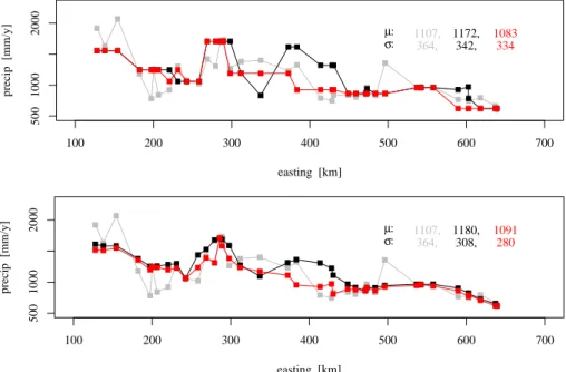
d -IDW interpolation are larger in mountainous terrain than in the lowlands (the same is valid for correlation and efficiency errors, not shown). In mountainous terrain the scatter in relative biases is smaller with γ- instead of d -interpolation and thus perfor-mance of γ-interpolation is better. This can also be seen in Fig.9. This figure shows interpolated precipitation sums in comparison with observed sums of 1999 in a
west-10
east transection with areal support of 350 to 370 km northing. Results with next- and four-neighbors interpolation are compared. Again the tendencies of over- and underes-timation of geographical or statistical distance interpolation are visible. The tendency of smaller values of statistical interpolation yields smaller standard deviations. Sub-jectively interpolation with n=4 leads to better results, but obviously also to smoother,
15
variability vastly underestimating fields.
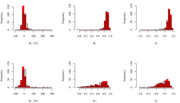
The smaller scatter in bias, correlation and efficiency by γ-IDW is also shown by the histograms in Fig.10. These histograms give statistics values applying n = 4 interpo-lation. The statistical distance interpolation is more robust than geographical distance interpolation. Extreme overestimates of daily means are avoided. Correlations are
20
shifted to higher values and the number of days with spatial R2≤0.5 and small or even useless (E ≤0) efficiencies are significantly reduced.
Obviously, time series performance is better than spatial performance. This is due to the scales of the data. The temporal support of the data is daily. The spatial support of the observations (∼1000 cm2) is very small in comparison (Orlanski, 1975). This
25
explains the better performance of interpolation in terms of time series than of spatial field comparisons. As a consequence the spatial results are more sensitive to the chosen interpolation method.
HESSD
2, 1893–1923, 2005Distance in spatial interpolation of daily
rain gauge data
B. Ahrens Title Page Abstract Introduction Conclusions References Tables Figures J I J I Back Close Full Screen / Esc
Print Version Interactive Discussion
EGU
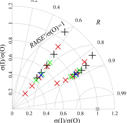
This is visualized in the Taylor (2001)-diagram shown in Fig. 11. For example, next-neighbor d -interpolation overestimates temporal and spatial variability in comparison with the evaluating observations. But, with n = 2, 4 etc. variability is more and more underestimated. This effect is more important for spatial than temporal variability be-cause of the relatively smaller spatial interpolation support scale. The traces of crosses
5
in the diagram are convex showing that there is an optimum number of neighbors to be considered in interpolation. If in the envisaged application the field correlation is more important than field variability then a number of four neighbors is well chosen in case of 50 observing stations. The optimum depends on the interpolation setup: number of stations, power of distance, spatial and temporal variability of the natural precipitation
10
field etc. The impact on smoothing of the power λ of the distance and de-skewing in γ-IDW are also shown in Fig.11. With increasing λ the effective number of observations decreases and variability of the interpolating values increases. De-skewing in γ esti-mation slightly improves variability, correlation and thus (as is proven inTaylor,2001) centered root-mean-square error RMSE0.
15
As discussed earlier there are systematic differences between station time series due to vertical or horizontal trends. In the interpolation experiments on a daily data basis these systematic effects are generally small in comparison to interpolation errors as is shown by application of γ0 instead of γ distances (cf. experiment γ0 in Table2). This says that on average the relative importance of vertical dependence of
precipita-20
tion rates is small in comparison with interpolation errors in our setup. Of course, in some areas or applications the vertical dependence is important. Additionally, these systematic effects get more important with increasing interpolation performance, for ex-ample because of increasing temporal support of interpolation time slices (i.e. monthly or yearly precipitation fields instead of daily fields).
25
Seasonal stratification of precipitation events in γ-estimation and -interpolation yields the expected results. Table2gives interpolation results if only summer or winter six-month data are considered (experiments Su and Wi). Spatial field correlations and efficiencies are better in winter than in summer. In Austria the winter precipitation is less
HESSD
2, 1893–1923, 2005Distance in spatial interpolation of daily
rain gauge data
B. Ahrens Title Page Abstract Introduction Conclusions References Tables Figures J I J I Back Close Full Screen / Esc
Print Version Interactive Discussion
EGU
intensive and less heterogeneous in the mean than summer precipitation. The more stochastic character of convective summer rain reduces the spatial representativeness of data. Nonetheless, the temporal correlation differences are small.
Interestingly, the temporal efficiencies are even better in summer than in winter. The MSEs of the interpolated time series are smaller in winter (d : 7.6 (mm/d)2 and
5
γ: 5.9 (mm/d)2) than in summer (d : 17.9 (mm/d)2 and γ: 15.9 (mm/d)2). But, if the MSEs are normalized with observed time series mean variance (22 and 66 (mm/d)2in winter and summer, respectively) then summer interpolation performs better than win-ter inwin-terpolation in win-terms of time series comparison. In either case, summer or winwin-ter, γ-IDW performs better than d -IDW with performance gain more pronounced in
win-10
ter because of higher stationarity of spatial patterns because of frontal interaction with orography.
We tried also stratification of precipitation days with a mean wind direction classifica-tion for the lower atmospheric levels in the Eastern Alps (Steinacker,1990). This even slightly reduces overall performance in γ interpolation. The small-scale γ-distances
15
are not highly dependent on large-scale wind direction. Additionally, the size of spe-cific wind direction classes is small even in the available thirty-year data sets and thus estimation of stratified γs is not robust.
5. Conclusions
Spatial interpolation of daily rain gauge data with Inverse Distance Weighting (IDW)
20
at locations with available precipitation time series has been investigated. It has been shown that the application of a statistical distance measure between neighbored precipitation time series instead of geographical distances between station locations slightly improves averaged interpolation performance. The main advantage is that sta-tistical distance IDW is more robust especially in or close to mountainous terrain where
25
complex rain-orography interaction is important that is implicitly considered in the sta-tistical distance. This performance gain in mountainous terrain illustrates the potential
HESSD
2, 1893–1923, 2005Distance in spatial interpolation of daily
rain gauge data
B. Ahrens Title Page Abstract Introduction Conclusions References Tables Figures J I J I Back Close Full Screen / Esc
Print Version Interactive Discussion
EGU
of simple but necessarily spatially highly resolving models of rain-orography interaction. The statistical distance could also be applied in geostatistical interpolation. For ex-ample, in Kriging interpolation n next neighbors are typically considered in estimation. These n neighbors could easily be selected by statistical distance. More sophisticated approaches could be thought of. For example, Kriging could be applied after mapping
5
station locations with statistical distances instead of geographical distances by metric multidimensional scaling (Sammon JR.,1969).
Implementation of IDW interpolation with statistical distance is easily done if the necessary time series are available at the interpolation sites. An example of application might be daily precipitation mapping in Austria. Operationally about 150 rain gauges
10
with daily or better resolution are available to the Austrian national weather service. FollowingWeilguni (2003) about 950 additional rain gauges with daily measurements are operated in Austria by the hydrological service, hydropower agencies etc. These additional stations are not available in near real-time, but their statistical information could be applied easily within the statistical IDW. This would be a parsimonious and
15
robust procedure for using all available rain gauge data in densification of the point data network that could be appropriately upscaled in precipitation mapping.
Acknowledgements. Data are provided by the Hydrographische Zentralb ¨uro, BMLFUW,
Vi-enna. The author is funded by the Austrian Academy of Sciences.
References 20
Adler, R. F., Kidd, C., Petty, G., Morissey, M., and Goodman, H. M.: Intercomparison of global precipitation products: The Third Precipitation Intercomparison Project (PIP-3), Bull. Amer. Meteor. Soc., 82, 1377–1396, 2001. 1894
Auer, I., B ¨ohm, R., Jurkovi´c, A., Orlik, A., Potzmann, R., Sch ¨oner, W., Ungersb ¨ock, M., Brunetti, M., Nanni, T., Magueri, M., Briffa, K., Jones, P., Efthymiadis, D., Mestre, O., Moisselin, J.-M.,
25
Begert, M., Brazdil, R., Bochnic ´ek, O., Cegnar, T., Gaji´c-Capka, M., Zaninovi´c, K., Majs-torovi´c, C., Szalai, S., Szentimrey, T., and Mercalli, L.: A new instrumental precipitation
HESSD
2, 1893–1923, 2005Distance in spatial interpolation of daily
rain gauge data
B. Ahrens Title Page Abstract Introduction Conclusions References Tables Figures J I J I Back Close Full Screen / Esc
Print Version Interactive Discussion
EGU
dataset for the greater Alpine region for the period 1800–2002, Int. J. Climatol., 25, 139–166, doi:10.1002/joc.1135, 2005. 1895
Barros, A. P. and Lettenmaier, D. P.: Dynamic Modeling of Orographically Induced Precipitation, Rev. Geophys., 32, 265–284, 1994. 1899
Beck, A. and Ahrens, B.and Stadlbacher, K.: Impact of nesting strategies on precipitation
5
forecasting in dynamical downscaling of reanalysis data, Geophys. Res. Lett., 31, pp. 5, doi:10.1029/2004GL020115, 2005. 1894
Bl ¨oschl, G. and Grayson, R.: Spatial observations and interolation, in: Spatial patterns in catchment hydrology: observations and modelling, edited by: Grayson, R. and Bl ¨oschl, G., Cambridge University Press, United Kingdom, 17–50, 2001. 1899
10
Ciach, G., Morrissey, M., and Krajewski, W. F.: Conditional bias in radar rainfall estimation, J. Appl. Meteorology, 39, 1941–1946, 2000. 1894
Daly, C., Neilson, R., and Phillips, D.: A statistical-topographic model for mapping climatological precipitation over mountainous terrain, J. Appl. Meteorology, 33, 140–158, 1994. 1896,1899 Frei, C. and Sch ¨ar, C.: A precipitation climatology of the Alps from high-resolution rain-gauge
15
observations, Int. J. Climatol., 18, 873–900, 1998. 1896
Haiden, T. and Stadlbacher, K.: Quantitative Prognose des F ¨achenniederschlags, ¨Osterr. Wasser- und Abfallwirtschaft, 10, 135–141, 2002. 1901
Orlanski, I.: A rational subdivision of scales for atmospheric processes, Bull. Amer. Meteor. Soc., 56, 527–530, 1975. 1904
20
Palecki, M. A., Angel, J. R., and Hollinger, S. E.: Storm precipitation in the United States. Part I: meteorological characteristics, J. Appl. Meteorology, 44, 933–946, doi: 10.1175/JAM2243.1, 2005. 1894
Rubel, F.: PIDCAP Quick Look Precipitation Atlas, vol. 15 of ¨Osterr. Beitr. Meteorol. Geophys., ZAMG, Wien, 1996. 1895
25
Rubel, F. and Hantel, M.: Correction of daily rain gauge measurements in the Baltic Sea drainage basin, Nordic Hydrology, 30, 191–208, 1999. 1896
Rubel, F. and Hantel, M.: BALTEX 1/6-degree daily precipitation climatology 1996–1998, Me-teorology and Atmospheric Physics, 77, 155–166, 2001. 1895,1896,1900
Rudolf, B. and Rubel, F.: Global precipitation, in observed global climate, edited by: M. Hantel,
30
Landolt-B ¨ornstein: Numerical Data and Functional Relationships in Science and Technology – New Series, Group 5: Geophysics Vol. 6, Subvolume A, 11.1–11.53, Springer, Berlin, 2005. 1896
HESSD
2, 1893–1923, 2005Distance in spatial interpolation of daily
rain gauge data
B. Ahrens Title Page Abstract Introduction Conclusions References Tables Figures J I J I Back Close Full Screen / Esc
Print Version Interactive Discussion
EGU
Sammon JR., J.: A nonlinear mapping for data structure analysis, IEEE Transactions on Com-puters, C-18, 401–409, 1969. 1907
Scheifinger, H., B ¨ohm, R., and Auer, I.: R ¨aumliche Dekorrelation von Klimazeitreihen unter-schiedlicher zeitlicher Aufl ¨osung und ihre Bedeutung f ¨ur ihre Homogenisierbarkeit und die Repr ¨asentativit ¨at von Ergebnissen, in Proceedings of 6. Deutsche Klimatagung,
Klimavari-5
abilit ¨at 2003, 22–25, September 2003, Potsdam, no. 6 in Terra Nostra, Schriftenreihe der Alfred-Wegener-Stiftung, 375–379, 2003. 1895
Sevruk, B.: Regional dependency of precipitation-altitude relationship in the Swiss Alps, Cli-matic Change, 36, 355–369, 1997. 1898
Shepard, D.: Computer mapping: the SYMAP interpolation algorithm, in: Spatial statistics and
10
models, edited by: Gaile, G. and Willmott, C., 95–116, Dordrecht: Reidel Publishing, 1984. 1899
Singh, V. and Frevert, D., eds.: Mathematical Models of Large Watershed Hydrology, Water resources Publications, LLC, Chelsea, Michigan, 2002a. 1894
Singh, V. and Frevert, D., eds.: Mathematical Models of Small Watershed Hydrology and
Appli-15
cations, Water resources Publications, LLC, Chelsea, Michigan, 2002b. 1894
Skoda, G., Weilguni, V., and Haiden, T.: Heavy convective storms – precipitation during 15, 60, and 180 minutes, chap. 2.5–7, Hydrological Atlas of Austria, Bundesministerium f ¨ur Land-und Forstwirtschaft, Umwelt Land-und Wasserwirtschaft, 2003. 1894
Smith, R.: The influence of mountains n the atmosphere, Adv. Geophys., 21, 87–230, 1979.
20
1899
Smith, R.: A linear upslope-time-delay model for orographic precipitation, J. Hydrology, 282, 2–9, 2003. 1899
Steinacker, R.: Eine ostalpine Str ¨omungslagenklassifikation, Tech. rep., IMG; Universit ¨at Wien, Austria,http://www.univie.ac.at/IMG-Wien/weatherregime/, pp. 8, 1990. 1906
25
Taylor, K.: Summarizing multiple aspects of model performance in a single diagram, J. Geo-phys. Res., 106, 7183–7192, 2001. 1905,1923
Tobler, W.: A computer movie simulating urban growth in the Detroit region, Economic Geogra-phy, 46, 234–240, 1970. 1896
Weilguni, V.: Precipitation stations, chap. 2.1, Hydrological Atlas of Austria, Bundesministerium
30
f ¨ur Land- und Forstwirtschaft, Umwelt und Wasserwirtschaft, 2003. 1907
Young, C., Nelson, B., Bradley, A., Smith, J., Peters-Lidard, C., Kruger, A., and Baeck, M.: An evaluation of NEXRAD precipitation estimates in complex terrain, J. Geophys. Res., 104,
HESSD
2, 1893–1923, 2005Distance in spatial interpolation of daily
rain gauge data
B. Ahrens Title Page Abstract Introduction Conclusions References Tables Figures J I J I Back Close Full Screen / Esc
Print Version Interactive Discussion
EGU
HESSD
2, 1893–1923, 2005Distance in spatial interpolation of daily
rain gauge data
B. Ahrens Title Page Abstract Introduction Conclusions References Tables Figures J I J I Back Close Full Screen / Esc
Print Version Interactive Discussion
EGU
Table 1. Statistics of the geographic distances of the considered station sets and statistics of
the common variance R2of daily precipitation series.
set distance (km) R2(%) min mean max min mean max
ALL/710 1 7 21 40 73 97
25 43 54 69 28 41 53
50 29 36 53 29 50 69
HESSD
2, 1893–1923, 2005Distance in spatial interpolation of daily
rain gauge data
B. Ahrens Title Page Abstract Introduction Conclusions References Tables Figures J I J I Back Close Full Screen / Esc
Print Version Interactive Discussion
EGU
Table 2. Mean evaluation results of interpolation experiments. The table gives the spatial mean
of relative time series biases Bt., the temporal mean of spatial biases is B.s, and the related
correlation coefficients Rt.and R.sand efficiencies. All values are given in percent and thus the
values of Bs would be 0 and all other values would be 100 in case of perfect interpolation. Exp. Bt. B.s Rt. R.s Et. E.s set,λ, n, − d /γ d /γ d /γ d /γ d /γ d /γ 25,2,4,− 1/−5 0/−7 84/85 56/60 67/71 22/33 50,2,4,− 4/−3 1/−7 87/88 62/65 73/76 32/42 150,2,4,− 1/−2 −1/−5 91/91 70/72 80/82 45/52 50,1,4,− 4/−2 1/−8 88/88 62/64 73/76 35/40 50,3,4,− 4/−3 2/−7 87/88 61/65 71/76 26/41 50,2,1,− 4/−2 4/−6 83/84 57/60 59/65 1/19 50,2,8,− 4/−3 1/−8 88/88 63/65 74/76 35/42 50,2,16,− 5/−5 1/−11 88/87 62/65 73/73 36/39 50,2,4,ln −/ 2 −/ 0 −/88 −/65 −/75 −/40 50,2,4,γ0 −/−3 −/−8 −/88 −/65 −/76 −/42 50,2,4,Wi 9/−5 0/−10 87/88 65/70 65/74 40/48 50,2,4,Su 2/−1 2/−6 87/88 60/61 73/76 25/36
HESSD
2, 1893–1923, 2005Distance in spatial interpolation of daily
rain gauge data
B. Ahrens Title Page Abstract Introduction Conclusions References Tables Figures J I J I Back Close Full Screen / Esc
Print Version Interactive Discussion EGU
0
1000
2000
3000
4000
0.0
0.2
0.4
elevation [mMSL]
rel. frequency
orography
all stations
50 stations
Fig. 1. Height distributions of the Austrian orography, of all considered rain gauges, and of a
HESSD
2, 1893–1923, 2005Distance in spatial interpolation of daily
rain gauge data
B. Ahrens Title Page Abstract Introduction Conclusions References Tables Figures J I J I Back Close Full Screen / Esc
Print Version Interactive Discussion
EGU
Fig. 2. Rain gauge locations of set ALL (bullets) considered in the present investigation and
measured values (bullet colors) for 19 August 1999. The orography is indicated by grey shading (light-grey: elevations above 800 m MSL, and dark-grey: elevations above 1500 m MSL). The main Austrian watersheds are indicated by black isolines.
HESSD
2, 1893–1923, 2005Distance in spatial interpolation of daily
rain gauge data
B. Ahrens Title Page Abstract Introduction Conclusions References Tables Figures J I J I Back Close Full Screen / Esc
Print Version Interactive Discussion EGU
0
500
1500
2500
0
1
02
03
04
0
elevation [mMSL]
precip [mm/d]
year 1999
day 19 August 1999
Fig. 3. Height dependence of precipitation observed by all stations for the year 1999 and the
HESSD
2, 1893–1923, 2005Distance in spatial interpolation of daily
rain gauge data
B. Ahrens Title Page Abstract Introduction Conclusions References Tables Figures J I J I Back Close Full Screen / Esc
Print Version Interactive Discussion EGU
0
100
200
300
400
500
0
100
150
d [km]
γ
[(
mm/d
)2
]
50
Fig. 4. Statistical distance γ for all evaluation-observation pairs. Here, 50 observing stations
are assumed. The γs for two stations (cf. the stations marked by colored arrows in Fig.7) are highlighted by colored symbols.
HESSD
2, 1893–1923, 2005Distance in spatial interpolation of daily
rain gauge data
B. Ahrens Title Page Abstract Introduction Conclusions References Tables Figures J I J I Back Close Full Screen / Esc
Print Version Interactive Discussion
EGU
Fig. 5. Relative representativeness in geographical (black bullets) and γ-statistical (red circles)
distance of the observing stations of set 50. The solid black and dashed red lines are local polynomial regression fits to the bullets and circles, respectively.
HESSD
2, 1893–1923, 2005Distance in spatial interpolation of daily
rain gauge data
B. Ahrens Title Page Abstract Introduction Conclusions References Tables Figures J I J I Back Close Full Screen / Esc
Print Version Interactive Discussion
EGU
Fig. 6. Relative importance of systematic differences between pairs of precipitation time series
over geographical distance between the series sites. The black dots show the relative impor-tance for station pairs with a vertical elevation difference of less than 50 m (only every 5th dot is drawn). The black circles show mean relative importances for geographical distance classes. The same is shown by the other colored symbols but for different vertical elevation difference classes.
HESSD
2, 1893–1923, 2005Distance in spatial interpolation of daily
rain gauge data
B. Ahrens Title Page Abstract Introduction Conclusions References Tables Figures J I J I Back Close Full Screen / Esc
Print Version Interactive Discussion
EGU
Fig. 7. IDW interpolation of data measured at 50 observing stations for 19 August 1999. The
color of the bullets at the station sites (marked with+) show the observed values. These are a subset of the observations shown in Fig.2. The squares indicate the interpolation points with the outline color giving the interpolation results by standard next-neighbor geographical IDW and the filling color giving next-neighbor γ-IDW results. The arrows point to the interpolation stations highlighted in Fig. 4. The circles mark observing stations not considered in next-neighbor γ-interpolation.
HESSD
2, 1893–1923, 2005Distance in spatial interpolation of daily
rain gauge data
B. Ahrens Title Page Abstract Introduction Conclusions References Tables Figures J I J I Back Close Full Screen / Esc
Print Version Interactive Discussion
EGU
Fig. 8. As Fig.7but showing precipitation sums for the year 1999 at 50 observation sites and relative biases at the evaluation sites. The vertical bars indicate relative biases for the 1999 interpolation experiments. The inlet shows the height of a bar with 100% positive bias. Black gives biases with geographical and red with statistical distance next-neighbor interpolation.
HESSD
2, 1893–1923, 2005Distance in spatial interpolation of daily
rain gauge data
B. Ahrens Title Page Abstract Introduction Conclusions References Tables Figures J I J I Back Close Full Screen / Esc
Print Version Interactive Discussion EGU 100 200 300 400 500 600 700 500 1000 2000 easting [km] precip [mm/y] µ : σ : 1107,364, 1172, 342, 1083 334 100 200 300 400 500 600 700 500 1000 2000 easting [km] precip [mm/y] µ : σ : 1107,364, 1180, 308, 1091 280
Fig. 9. Year 1999 sums of observed and interpolated precipitation at sites in a west-east
tran-section with areal extent between 350 and 370 km northing. Grey symbols show the observed values, black symbols the interpolated values with geographical distance interpolation and red symbols with statistical distance interpolation, respectively. The upper panel applies n=1, i.e. next-neighbor, and the lower panel applies n=4 neighbors in interpolation. The transection means µ and standard deviations σ are given too.
HESSD
2, 1893–1923, 2005Distance in spatial interpolation of daily
rain gauge data
B. Ahrens Title Page Abstract Introduction Conclusions References Tables Figures J I J I Back Close Full Screen / Esc
Print Version Interactive Discussion EGU Bt. [%] frequency −100 0 100 200 300 0 5 0 100 150 Rt. frequency 0.0 0.2 0.4 0.6 0.8 1.0 0 5 0 100 150 Et. frequency −1.0 −0.5 0.0 0.5 1.0 0 5 0 100 150 B.s [%] frequency −100 0 100 200 300 0 5 0 100 150 R.s frequency 0.0 0.2 0.4 0.6 0.8 1.0 0 5 0 100 150 E.s frequency −1.0 −0.5 0.0 0.5 1.0 0 5 0 100 150
Fig. 10. Histograms of spatially (upper row) and temporally (lower row) averaged statistics.
The solid red histograms show the evaluation results for γ- and the hatched black histograms for the d -distance interpolation with set 50, n=4, and γ=2.
HESSD
2, 1893–1923, 2005Distance in spatial interpolation of daily
rain gauge data
B. Ahrens Title Page Abstract Introduction Conclusions References Tables Figures J I J I Back Close Full Screen / Esc
Print Version Interactive Discussion EGU
R
σ(I)/σ(O)
σ(I)/
σ(O)
RMSE'/
σ(O)
=1
Fig. 11.Taylor(2001)-diagram showing evaluation results with observation set 50 but different interpolation setups. Black “+” and red “x” show the dependency on n with n=1, 2, 4, 8, 16 for
d - and γ-interpolation, respectively, and γ=2. The green “x” show results with γ-interpolation
and n=4 and γ=1, 3, 4. The blue “x” show results for experiment ln. The group of symbols indicating better correlations and centered RMSE0s are from time series comparisons and the other group indicate spatial field comparisons.