Quantification of mesoscale transport across the boundaries of the free troposphere: a new method and applications to ozone

HAL Id: hal-00327929

https://hal.archives-ouvertes.fr/hal-00327929

HAL is a multi-disciplinary open access

archive for the deposit and dissemination of sci-entific research documents, whether they are pub-lished or not. The documents may come from teaching and research institutions in France or abroad, or from public or private research centers.

L’archive ouverte pluridisciplinaire HAL, est destinée au dépôt et à la diffusion de documents scientifiques de niveau recherche, publiés ou non, émanant des établissements d’enseignement et de recherche français ou étrangers, des laboratoires publics ou privés.

Quantification of mesoscale transport across the

boundaries of the free troposphere: a new method and

applications to ozone

F. Gheusi, Jean-Pierre Cammas, F. Cousin, C. Mari, P. Mascart

To cite this version:

F. Gheusi, Jean-Pierre Cammas, F. Cousin, C. Mari, P. Mascart. Quantification of mesoscale transport across the boundaries of the free troposphere: a new method and applications to ozone. Atmospheric Chemistry and Physics Discussions, European Geosciences Union, 2004, 4 (6), pp.8103-8139. �hal-00327929�

ACPD

Print Version Interactive Discussion

EGU

Atmos. Chem. Phys. Discuss., 4, 8103–8139, 2004 www.atmos-chem-phys.org/acpd/4/8103/

SRef-ID: 1680-7375/acpd/2004-4-8103 European Geosciences Union

Atmospheric Chemistry and Physics Discussions

Quantification of mesoscale transport

across the boundaries of the free

troposphere: a new method and

applications to ozone

F. Gheusi, J.-P. Cammas, F. Cousin, C. Mari, and P. Mascart

Laboratoire d’A ´erologie, Toulouse, France

Received: 17 September 2004 – Accepted: 27 October 2004 – Published: 8 December 2004 Correspondence to: F. Gheusi ([email protected])

ACPD

Print Version Interactive Discussion

EGU

Abstract

A new Lagrangian method is proposed to quantify the transport of ozone – or any other atmospheric constituent – by objectively-defined air-masses. In the framework of mesoscale modelling, this method is an alternative to classical Eulerian or trajectory-based methods, which suffer from many drawbacks at this scale. The elementary

5

air-parcels are tagged with their initial location (what is made possible in the model by passive transport of three tracer fields initialized with the space coordinates). This enables to retrieve not only their back-trajectories but also their physical and chemical history. This information is in turn used to relevantly define transporting air-masses along objective criteria. For instance the ozone mass that has left the planetary

bound-10

ary layer (PBL) to intrude the free troposphere (FT) in a given time interval, is carried by the ensemble of air-parcels that were initially in the PBL but are finally in the FT. Such an air-mass can be characterized by e.g., a criterion on the initial and final values of the turbulent kinetic energy of the air-parcels. The last step to obtain the sought ozone mass is a simple spatial integration of the ozone concentration over the so-defined

15

air-mass. Two case-studies are presented as illustrations with increasing complexity: (i) the downward transport of ozone accompanying a tropopause fold, across a mid-tropospheric altitude level; (ii) a case of PBL-to-FT transport, as evoked above.

1. Introduction

Tropospheric ozone is not only a major atmospheric photo-oxidant but also the third

20

most active greenhouse gas after carbon dioxide and methane (IPCC,2001). Its radia-tive impact is maximum in the upper troposphere (de Forsters and Shine,1997) where it even equals that of the carbon dioxide (Micley et al.,1999). It is thus crucial to ac-quire a quantitative and comprehensive knowledge of the terms of its budget in order to understand the mechanisms of its variability at the various spatial (local, regional,

25

ACPD

Print Version Interactive Discussion

EGU

This budget of tropospheric ozone still remains quantitatively very uncertain and dif-ficult to establish due to its high photochemical reactivity and the fact that this gas is not directly released in the atmosphere but produced in-situ by chemical cycles including various precursor species as organic compounds, nitrogen oxides, etc. Especially at the global scale with up-to-date chemistry-transport numerical models (CTMs) there is

5

still a great dispersion of the terms of stratospheric ozone influx into the troposphere and surface deposition. That dispersion appears to be “sponged” by the modelled chemical cycles. As a result the simulated photochemical net production turns out to be either positive or negative according to various models (IPCC,2001).

Contributing especially to the complexity of the problem, it is established that the

10

kinetic regimes of chemical ozone production/loss in the planetary boundary layer (thereafter PBL) and free troposphere (thereafter FT) are very different due to con-trasting dilutions of precursors and non-linear sensitivity on their concentrations. CTMs poorly capture this difference and this problem will persist as long as ozone exchanges through the boundaries of the PBL and FT are not correctly represented in the models

15

– even with the best possible chemical scheme.

More specifically the question of free-tropospheric ozone has become in the last years a major concern in the scientific community. The background ozone concentra-tion has notably increased whereas the urban precursor emissions and local ozone pollution peaks have decreased past the last decade in the developed countries. Thus

20

the problem of ozone pollution is shifting from a local to a global issue. In particu-lar long-range transport and slow ozone production in the free troposphere are now recognized to take an important part in regional budgets (e.g.,Chattfield et al.,2004;

Sauvage et al.,2004).

As the ozone budget of the free troposphere is significantly controlled by exchange

25

processes at its upper and bottom boundaries, one has to be able to assess these exchanges precisely. A difficulty is that most of these exchange processes occur at scales meso-α, -β or even finer. Another major difficulty is that the crossed dynamical boundaries – the tropopause and the PBL top – are highly deformable and unstationary,

ACPD

Print Version Interactive Discussion

EGU

and are not defined by a geometrical but physical criterion – for instance on potential vorticity (PV) and turbulent kinetic energy (TKE), respectively.

Although not impossible it is uneasy to express mass fluxes across such complex surfaces in the form of a diagnostic formula based on the Eulerian flow variables. Wei

(1987) proposed a formula for flux estimate across the tropopause based on the

conti-5

nuity equation. This formula (seeKowol-Santen et al.,2000, Eq. 2), takes into account the vertical velocity at the tropopause, the local vertical change of the tropopause po-sition and the isentropic transport across the tropopause. A simple form is attained only if PV is taken as vertical coordinate (seeKowol-Santen et al.,2000, Eq. 3). This however requires everywhere a one-to-one correspondence between PV and altitude,

10

which is in general not the case in mesoscale modelling – of a tropopause fold for instance. The flux fields derived from the formula in its general form suffer from small-scale noise due to horizontal spatial derivatives (Wirth and Egger,1999) all the more as the model horizontal resolution is fine.

Thus in the recent years most quantitative studies on stratosphere-troposphere

ex-15

changes (thereafter STE) preferred Lagrangian approaches using various techniques. The most common is based on the computation of large gridded ensembles of trajec-tories, with automatic selection of those corresponding to pre-defined STE events. The exchange assessment (in terms of mass of dry air, ozone, etc.) relies on the assump-tion that each parcel transport a fixed (finite) mass or volume of air – that of a grid-cell.

20

As trajectories can be computed from pre-existing global meteorological analyses, this technique has been used to establish climatologies of STE events and accompanying mass fluxes at the hemispheric scale (e.g., Sprenger and Wernli, 2003; Stohl et al.,

2003). However Gheusi and Stein (2002) pointed out limitations of trajectory-based analyses (in particular resulting from time and space interpolations of coarse wind

25

fields, and the absence of sub-grid transport parametrization in the trajectory computa-tion) and stressed that these limitations can be critical for studies at mesoscale. More-overStohl et al.(2004) recently warned on the dynamical inconsistency of subsequent analysed wind-fields as a source of exchange overestimation.

ACPD

Print Version Interactive Discussion

EGU

The isentropic and quasi-horizontal stretch and cut-off of stratospheric PV-filaments from high to sub-tropical latitudes has been identified as a major process of ST ex-change. Even if such filaments often extend over thousands kilometres, they can be as thin as few tens kilometres due to intense stretching in baroclinic wave developments at mid-latitudes. Based on the assumption of PV conservation in adiabatic inviscid

5

flows, the technique of PV-contour advection on isentropic surfaces allows to generate small-scale features from initially coarse PV fields from meteorological analyses and to simulate the evolution of stratospheric filaments with some realism.Dethof et al.(2000) proposed an algorithm based on this technique to calculate mass budgets across the tropopause. A “surgery” routine is used to remove small-scale structures by merging

10

or disconnecting contours if they get closer than a specified cutoff scale. Stratospheric intrusions are thus allowed to cut off from the polar stratospheric reservoir then a sim-ple mass integration is finally performed to assess the accompanying stratosphere to troposphere exchange. The above method of cross-tropopause transport quantifica-tion relies however on the limiting assumpquantifica-tions of quasi-horizontal, adiabatic, inviscid

15

flow – not always fulfilled e.g., in extra-tropical cyclones that are the most favourable conditions for ST transports.

Although the above Lagrangian methods to asses ST exchanges are quite different in their details, they can all be outlined along a single two-step process:

1. Identification of coherent air-masses (stratospheric filaments, tropopause folds,

20

cumulonimbus overshoots, etc.) that (more or less irreversibly) intrude into, or extrude from, the troposphere;

2. Quantification of the mass of dry air, ozone, or any other atmospheric constituent, transported by these air-masses.

It should be noted that the same two-step process can be followed to quantify

trans-25

ports from the planetary boundary layer into the free troposphere – or conversely. In the present paper a new method is proposed to assess the transport of atmo-spheric constituents – focusing on ozone as an example – across the boundaries of the

ACPD

Print Version Interactive Discussion

EGU

free troposphere in the framework of numerical-model based studies at scales meso-α, -β, or even below, where the limitations of the Lagrangian techniques mentioned above become critical.

Also following the above two-step process, the new method is based on the tech-nique of Lagrangian analysis using Eulerian passive tracers developed byGheusi and

5

Stein (2002). Its use does not require any constraining assumption (such as adiabatic or inviscid flow, PV conservation, etc.) and has proven its efficiency to identify, track and study mesoβ-scale coherent air-masses in complex situations (e.g.,Gheusi and

Stein,2002;Asencio et al.,2003;Cousin et al.,2004).

Thus this Lagrangian technique appears to be of immediate applicability for step 1

10

of the quantification process when considering transports by mesoscale air-masses into or from the free troposphere. So the main objective of the paper is to define a procedure for step 2. Two examples of increasing complexity will be given to show how to quantify ozone transports into the free troposphere by a tropopause fold and a boundary-layer plume, respectively.

15

The remainder of the paper is structured as follows. In Sect. 2 the model specifi-cations will be briefly given. Some aspects of the Lagrangian analysis technique of

Gheusi and Stein (2002) will be also recalled, that are essential to understand the whole transport quantification process. In Sect. 3 the method will be carried out in a simple configuration to assess a descending time-integrated ozone flux associated to

20

a tropopause fold across a fixed altitude level. In Sect. 4 a more complex situation of BL ozone plume is considered where the crossed surface is the PBL top defined with a given value of the turbulent kinetic energy. Some aspects of the method (errors, calibration, advantages) are discussed in Sect. 5. Conclusions are given in Sect. 6.

ACPD

Print Version Interactive Discussion

EGU

2. Model specifications and Lagrangian technique

2.1. Model specifications

The numerical simulations are performed with MesoNH – a non-hydrostatic anelastic mesoscale model jointly developed by the Laboratoire d’A ´erologie (Toulouse, France) and the CNRM (M ´et ´eo-France). The configurations of MesoNH used in Sects. 3 and 4

5

differ in terms of model domain, resolution, microphysics and ozone chemistry. Specific details will be introduced in the respective sections. The main common features are given below.

The dynamical core of the model is described in Lafore et al. (1998). A terrain-following vertical coordinate is used to include orography, based on altitude levels

10

and the Gal-Chen and Sommerville (1975) transformation. Subgrid turbulence is parametrized with a 1-D, 1.5-order scheme using the turbulent kinetic energy as prog-nostic value (Cuxart et al., 2000) and the Bougeault and Lacarr `ere (1989) vertical-mixing length.

The warm-cloud microphysics scheme is of Kessler (1969) type including water

15

vapour and liquid water in the form of non-precipitating cloud droplets or rain. Sub-grid convection is parametrized with a 1-D massflux scheme (Bechtold et al., 2001). The surface scheme is “Interactions between the Soil, Biosphere and Atmosphere” (ISBA, Noilhan and Planton, 1989). The radiation scheme is described in Morcrette

(1991).

20

A complete set of references and comprehensive documentations can be found on the official MesoNH web site (http://www.aero.obs-mip.fr/mesonh/).

Initialization and coupling at the model boundaries for the meteorological fields is realized from French operational analyses ARPEGE (Th ´epaut and Coauthors,1998). The model also include mixing ratios of chemical species that are either treated as

25

passive tracers (Sect.3) or evolve according to a chemical scheme (Sect.4). In both cases chemical mixing-ratio fields for initialization and coupling result from the CTM at

ACPD

Print Version Interactive Discussion

EGU

global scale MOCAGE developed by M ´et ´eo-France (Cathala et al.,2003). 2.2. Lagrangian technique

The Lagrangian technique used in this paper is here only briefly recalled. Full details and discussions can be found inGheusi and Stein(2002) and Gheusi and Stein (2004, personal communication1).

5

The Lagrangian description of a flow consists in specifying for each elementary fluid parcel (hereafter referred to as a Lagrangian parcel), and at any time, its location as well as any quantities (velocity, pressure, temperature, chemical species concentra-tions, etc.) characterizing the parcel properties. This requires that each Lagrangian parcel has to be labelled so that its identity remains unambiguous. A possible way is

10

to label each parcel with its location, say x₀, at an arbitrary reference time t₀.

Like most fluid-dynamics numerical models, MesoNH is formulated with differential equations operating on Eulerian fields. In this framework it is in fact very easy to make such a labelling, based on the transport of passive scalar variables – a very common task in numerical modelling. The method consists, at an arbitrary reference time t₀, in

15

initializing three fields of passive scalars with the three space coordinates, namely:

x₀(x, t₀)= x,

y₀(x, t₀)= y,

z₀(x, t₀)= z.

Since these fields (hereafter referred to as the “initial coordinates”) are passive

20

scalars driven by the flow, their evolution is governed by the advection equation

∂x₀

∂t = −u · ∇x0, (1)

where u is the velocity field and x₀(x, t) is the vector field formed with the compo-nents x₀, y₀, z₀. The discretization of Eq. (1) in finite elements implies that the three

1

ACPD

Print Version Interactive Discussion

EGU

passive-tracer fields experience not only advection but also the sub-grid turbulent and convective transports through the corresponding parametrizations.

It should be remarked that conservation of the initial coordinates is assumed by definition and is free of constraining hypotheses (like adiabatic or inviscid flow, PV conservation, etc.) so that this Lagrangian technique can be used in the most complex

5

meteorological situations at mesoscale.

Thus at any time t>t₀, x₀(x, t) provides the location at time origin t₀of the air-parcel that is now at location x. This is immediately useful for studying mesoscale exchanges since air-masses intruding from an atmospheric reservoir to another appear on initial coordinate fields as coherent ensembles with a common geographical origin.

10

Another straightforward consequence is that for instance the initial potential vorticity

P V₀ (or any other quantity) that the considered Lagrangian parcel had at time origin

t₀can be simply known by reading the (Eulerian) P V field at time t₀ and location x₀:

P V0=P V (x0, t₀), or in the fully developed Eulerian form

P V₀(x, t)= P V (x0(x, t), t₀). (2)

15

This will be useful to discriminate air-parcels originating from reservoirs defined along physical criteria. For example, if the stratosphere is defined at time t₀ as the region with P V >2 PVU, at time t>t₀ any air-parcel in the troposphere with P V₀>2 PVU is

im-mediately identified as a parcel originating from the stratosphere2.

3. Transport across a fixed horizontal surface

20

In this section we consider a case of ozone import in the troposphere by a tropopause fold that is known to be among the main processes that contribute to the global

de-2

This technique is close to the “Reverse Domain Filling” (RDF, e.g.,Schoeberl and Newman,

1995). However the reconstructed potential vorticity field P V₀is here not obtained by means of an ensemble of backtrajectories but the reconstruction is based on the initial location (Eulerian) field x₀(x, t).

ACPD

Print Version Interactive Discussion

EGU

scending stratospheric ozone flux at extra-tropical latitudes.

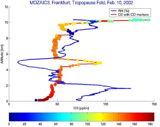
The fold was present on 10 February 2002 over western Europe and was detected by a commercial aircraft A340 instrumented with MOZAIC sensors (N ´ed ´elec et al.,

2003) that took off from Frankfurt (Germany) on the same day. It is well visible in ozone (O₃), carbon monoxide (CO) and humidity vertical profiles (Fig.1) as an O₃-rich,

CO-5

poor and dry thin layer between altitudes of 4 and 5 km. The fold accompanied the development of a classical extra-tropical baroclinic-wave over eastern Atlantic.

3.1. Tropopause fold simulation and validation

The considered case of winter extra-tropical wave development necessitates that the model microphysics also includes three iced-phase species (non-precipitating cloud

10

particles, snow flakes and graupels) following the “Ice3” scheme (Pinty and Jabouille,

1998).

The life-time of ozone in the upper troposphere in winter at mid and high latitudes is estimated to several weeks (von Kuhlmann et al.,2003). The simulation presented in this section runs over 48 h so that chemical reactions including ozone have been

15

neglected and that gaseous constituent is treated in the model as a passive tracer. The model domain extends over 3000 km meridionally and 4500 km zonally in polar strereographic projection, and covers eastern Atlantic and western Europe with a hori-zontal resolution of 30 km. The model has 82 vertical levels with 40 m of resolution near the ground progressively stretched to 300 m at 3000 m. Above this altitude it remains

20

constant up to the model top at 20 000 m.

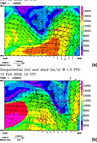
The model was initialized on 9 February 2002 00:00 UTC. Figure2shows the altitude of the 1.5 PVU PV-isopleth on 9 February at 18:00 UTC and 10 February at 12:00 UTC. On this surface the baroclinic wave appears as a deep (2000 m at least) V-shaped trough moving rapidly eastward while elongating southward and narrowing.

25

In case of multiple occurrence of the 1.5 PVU value on a given vertical, only the highest point of the PV-isopleth is represented in Fig.2. This is the case in panel (b) near the western edge of the trough where tropopause folding has occurred – visible

ACPD

Print Version Interactive Discussion

EGU

as a discontinuity of the surface altitude (sudden drop from 10 000 m down to below 7000 m) just east of Frankfurt.

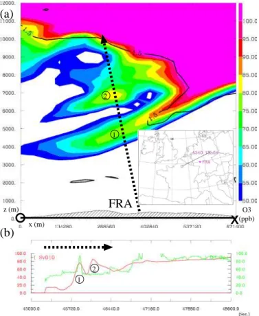
The vertical structure of the modelled fold in PV and O₃ mixing-ratio not far NW of Frankfurt is shown in Fig.3a. Airborne O₃measurements have also been emulated in the model along the path of the MOZAIC aircraft. The real and simulated records are

5

plotted together in Fig. 3b. In the model two ozone-rich layers (marked 1 and 2) are intercepted by the ascending aircraft (Fig.3a) with their corresponding O₃peaks well visible in the simulated record (red curve in Fig.3b).

The O₃ layer 1 is associated to the tropopause fold (as shown by the coincidence with the overturned PV-contour). Compared to the measurements (green curve in

10

Fig.3b) it is captured by the model at the right altitude and with satisfying amplitude and thickness (given the coarser vertical resolution of the model, 300 m, with respect to that of the measurements, about 30 m). In contrast the simulated feature 2 was not actually measured by the aircraft and there is also an underestimation of O₃ concen-tration below 4000 m. Nevertheless only the ozone intrusion due to the fold is under

15

consideration in this study and the present simulation appears to be satisfying for the goal of quantifying the accompanyning transport of O₃.

3.2. Downward transport quantification

The purpose in this subsection is to quantify the transport of ozone specifically as-sociated to the tropopause folding process and accompanying subsident air motion.

20

Precisely we seek to asses the mass of O₃ (in kg) crossing downward a reference altitude level, z=4500 m, during a given time period starting (arbitrarily) on 9 Febru-ary 18:00 UTC. This mass therefore corresponds to a time-integrated mass-flux of O₃ through that level. The reference altitude is chosen sufficiently low in the troposphere to consider that this deep intrusion of stratospheric ozone is irreversible.

25

The process for that quantification has two stages: (i) to select objectively the ozone-carrying air-mass that has crossed downward the reference level during the 18 h period from 9 February 18:00 UTC to 10 February 12:00 UTC; (ii) to perform a volume

inte-ACPD

Print Version Interactive Discussion

EGU

gration over this air-mass to assess the total ozone mass transported in it. 3.2.1. Air-mass selection

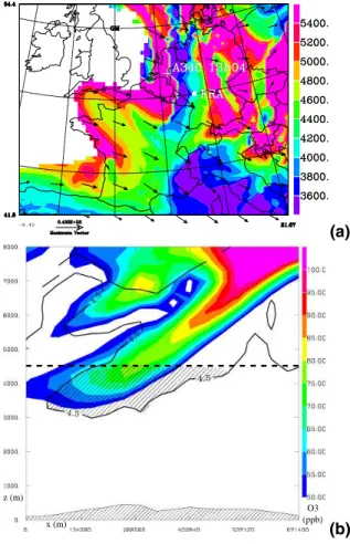
The first stage is based on the tracer field of initial altitude, z₀(x, t) (see Sect. 2.2). Isopleths of this field correspond to surfaces that are initially horizontal at the time-origin, then materially deformed by the flow. Such a surface is represented seen from

5

above in Fig.4a. This shows the actual altitude after 18 h, of the points of the surface that were initially at 4500 m. This plot evidences the subsiding motion of air-parcels accompanying the tropopause folding process, down to altitudes as low as 3600 m (NS-oriented band in the blue-purple range, extending from north-eastern France to the North Sea). A vertical section (Fig.4b) further illustrates the downward deformation

10

of the material surface (visible as a contour) in the region of the ozone intrusion (and even shows that the z₀-surface itself has folded). Thus the z₀ field allows to outline vertical displacements integrated over the chosen time period.

This can serve to select objectively a descending air-mass as follows. Clearly all the air-parcels that were initially above 4500 m and are now below, have crossed downward

15

the altitude level 4500 m. It is in fact very easy to formulate this criterion by means of the initial altitude field, which is fulfilled for any air-parcel present at time t at location x=(x, y, z) if, and only if,

z≤ 4500m .AND. z₀(x, t) ≥ 4500m. (3)

In Fig.4b this statement is true for the whole air-mass located below 4500 m but above

20

the z0=4500 m isocontour (hatched area).

Finally we further restrict the selected descending air-mass within an arbitrary ge-ographical domain represented in Fig.5a, in order to filter any downward transport in the model domain not associated to the tropopause fold.

ACPD

Print Version Interactive Discussion

EGU

3.2.2. Mass integration

Figure 5 shows a field equal to the O₃ mixing-ratio field where the above criterion (3) is fulfilled, and zero elsewhere. This three-dimensional field (noted [O₃]_↓) hence represents the ozone distribution restricted to that transported downward through the 4500 m altitude level since the time origin. It is now straightforward to assess the total

5

ozone mass contained in the selected air-mass by simple integration over space: Z Z Z [O₃]_↓ M_O 3 M_{ai r} ρai rdV, where M_O

3 and Mai r are the molar mass of ozone and air (48 and 29 g/mol,

respec-tively), ρ_{ai r} the density of air and dV a volume element.

The discretized calculation from the model fields is performed as follows. The above

10

criterion is tested at each model grid-point, producing a three-dimensional binary ar-ray where the 0/1 (false/true) transition surface is a pixelized contour encompassing the selected air-volume. This contour is smoothed by application in each direction of space, of a running-mean operator with weight 1₂ for the local grid point and 1₄ for the two adjacent points. As a result the transition region appears as “grey” values (i.e.,

15

continuously between 0 and 1). Finally only the model cells where this truth-indicator equals or exceeds the threshold α=0.57 are kept as finite volume-elements for the integration3.

In the considered example this yields a mass of ozone of 19.4 106kg in 18 h for this single ozone intrusion event. Estimations given in the literature for daily ozone

20

quantities transported across the tropopause into the troposphere by single tropopause events were gathered byBeekmann et al.(1997). Those range between 1.8 and 10.4 1032 molecules per day (molec/d). The mass found above for an 18 h period corre-sponds to a mean rate of 3.3 1032molec/d, well within that range of values.

3

ACPD

Print Version Interactive Discussion

EGU

It is noteworthy that the latter downward flux across the 4500 m altitude level is found to have the same order of magnitude as those estimated across the tropopause. This illustrates that tropopause folds should be considered as deep and bursty injections of ozone into the troposphere, and thus points out a severe limitation of flux-type for-mulations at the tropopause level for the tropospheric forcing in large-scale long-range

5

models of tropospheric ozone. Further discussion on that topic is however beyond the goals of the present study.

Regarding the method itself, its advantages in a so basic case – a flux through a horizontal fixed surface – compared to a classical on-line Eulerian method will be discussed in Sect. 5but before a much less trivial case is presented in the following

10

section.

4. Transport across an unstationary complex surface

As stressed in Sect. 1, it may be uneasy to express mass fluxes across complex un-stationary surfaces, based on the Eulerian flow variables, so that Lagrangian methods are often preferred. This is the case here where the considered surface is the top of

15

the boundary layer, defined by a threshold value on the turbulent kinetic energy (TKE). The chosen meteorological situation is a summer sunny day on the Mediterranean coast where a marked diurnal cycle and the development of coastal breezes render the boundary layer particularly unstationary and complex.

4.1. Model configuration and meteorological situation

20

The model configuration was designed for the study of summer ozone-pollution episodes in the boundary layer in the region of Marseille during the ESCOMPTE cam-paign in 2001 (Cousin et al.,2004). The 720 km×720 km model domain is centred over the north-western Mediterranean basin (Gulf of Lion) and includes part of the French and Spanish surrounding coasts and mountains (eastern Pyrenees, southern Massif

ACPD

Print Version Interactive Discussion

EGU

Central and southwestern Alps) with a horizontal resolution of 9 km. The model has 54 vertical levels with 10 m of resolution near the ground progressively stretched to 1500 m at 10 000 m. Above this altitude it remains constant up to the model top at 15 000 m. The chemical evolution of ozone mixing-ratio is taken into account through the chemistry module ReLACS (Crassier et al.,2000;Tulet et al.,2003) derived from

5

RACM (Stockwell et al.,1997). ReLACS operates on 128 chemical reactions involving 37 gaseous species, and is coupled on-line with Meso-NH. More details on the spe-cific design of the model for the ESCOMPTE campaign are provided byCousin et al.

(2004).

The situation considered here is the afternoon of 23 June 2001. A high-pressure

10

regime was well established over the Gulf of Lion and nearby, with sunny weather and a gentle WNW’ly synoptic flux (of about 15 m/s) in the mid-troposphere (Fig.6a). Such conditions dominated by radiation were very favourable to the development in the afternoon of mountain- and sea-breeze in the lowest levels (below 200 m a.s.l.) all along the coast of the Gulf of Lion (see Figs. 6b and 9a). A deep boundary layer

15

(exceeding 2000 m) has formed above the relief, and especially along the convergence line delimiting the penetration of the breeze inland (Fig.6b and9a). It is fully developed around 15:00 UTC then rapidly collapses after 17:00 UTC (in the same time as the breeze circulation).

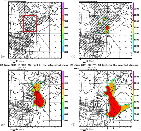
The ozone mixing-ratio field together with a marker of the boundary layer – defined

20

as T K E ≥0.2 m2/s2 (about 10% of typical values for a well-developed boundary layer) – are displayed at z=2000 m in Fig.7at the climax of the boundary layer development (15:00 UTC), then few hours later in the early evening (20:00 UTC). At 15:00 UTC ozone-laden air (mixing-ratio above 70 ppbv) is well correlated with the boundary layer where developed up to 2000 m or above. This distribution is clearly due to turbulent

up-25

ward transport of ozone photochemically formed in polluted air at lower levels in the few past hours. At 20:00 UTC the boundary layer has almost everywhere collapsed below 2000 m but the ozone-rich air mass is still present at this altitude and has been trans-ported over the Mediterranean over few tens kilometres by the north-westerly wind.

ACPD

Print Version Interactive Discussion

EGU

The depicted situation illustrates how an ozone-rich air-mass can be formed in the boundary layer then be released into the free troposphere where it may then experi-ence transport over a more or less long range. The next subsection is devoted to the quantification of this ozone transfer from the boundary layer to the free troposphere. 4.2. Transport quantification through the PBL-top up to the free troposphere

5

As in previous Sect.3 the two-step process will be followed, with first an appropriate and objective selection of the transporting airmass, then the integration of the ozone amount over this airmass.

Our objective is to asses the total ozone mass that has crossed upward the top of the boundary layer (hereafter PBL-top) since the reference time t0=15:00 UTC. Here

10

we consider the PBL-top to be the surface defined at any instant by the threshold value

T K E=0.2 m2/s2.

4.2.1. Air-mass selection

Any air-parcel that has crossed the PBL-top since the time origin t₀was in the PBL at

t₀and is now in the free troposphere. In other words its TKE was above 0.2 m2/s2at t₀

15

and is now (time t) below. The transporting airmass is thus formed by the ensemble of air-parcels that fulfil this criterion.

Recalling Eq. (2) (Sect.2.2), the air-parcel at current time t and location x had at t₀ a turbulent kinetic energy

T K E₀= T K E(x0(x, t), t₀).

20

The transporting airmass is thus defined by the conditions:

T K E (x, t) ≤ 0.2 m2/s2 (4) .AND.

ACPD

Print Version Interactive Discussion

EGU

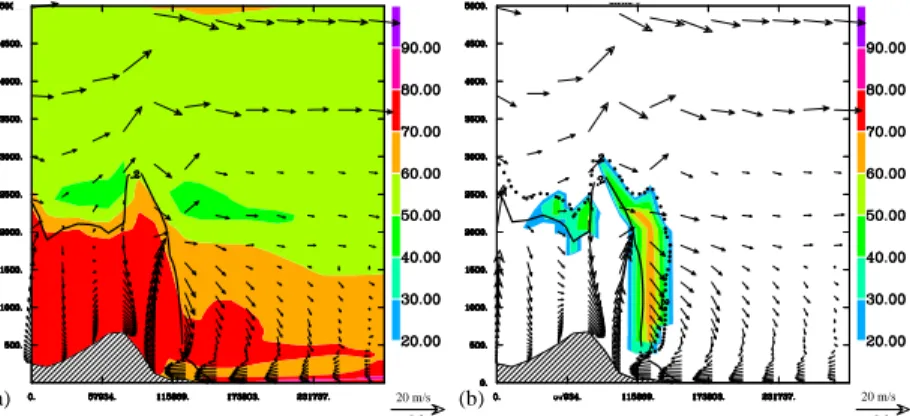
It is also possible to further specify the definition of the airmass with an added geo-graphical criterion, for example to restrict to air initially present over the southern Massif Central within the box drawn in Fig.8a. The geographical added condition is thus:

x_min≤ x₀(x, t) ≤ x_max.AND. y_min ≤ y₀(x, t) ≤ y_max, (6) (where x_min, x_max, y_min, y_max, are the coordinates specifying the box in Fig.8a).

5

The airmass defined along the criteria of Eqs. (4), (5) and (6), is shown at several instants at z=2000 m in Figs. 8b–d, and in vertical section in Figs. 9b–d. More pre-cisely the represented field is the ”selected” ozone mixing-ratio (hereafter noted [O₃]_↑), obtained by multiplication of the mixing-ratio field by 1 where the above criteria are fulfilled, and by 0 elsewhere.

10

In these figures also appear the fields T K E and T K E₀ used to define the airmass. The contour T K E=0.2 m2/s2is represented at the initial time t₀(Fig.8a) then the coun-tour T K E0=0.2 m2/s2 at later instants, so that the south-eastward transport of the air parcels that initially formed the PBL-top is well visible over the Gulf of Lion (Fig.8b–d). Current values of T K E above 0.2 m2/s2 – i.e., parcels still in the PBL – are also

indi-15

cated (hatched area). Therefore [O₃]_↑appears to be non-zero inside the T K E₀contour (parcels that were in the PBL) but outside the hatched area (parcels that are no more in the PBL).

4.2.2. Mass integration

Again a volume integral over the selected air-mass finally yields the expected result –

20

namely the total mass of ozone that originates from the box over the southern Massif Central and has crossed upward the PBL-top since the reference time t₀:

Z Z Z

[O₃]_↑ MO3

ACPD

Print Version Interactive Discussion

EGU

In the same vein the total mass of air in the selected volume is: Z Z Z

δ_↑ρ_{ai r}dV,

where δ_↑is 1 in the selected volume and 0 elsewhere.

The numerical integration again follows the procedure described in Sect. 3.2.2. The obtained ozone mass at 20:00 UTC amounts to 1.60 106kg, the air mass to

5

1.36 1013kg.

These numbers mean little by themselves since the way to define the air-mass was arbitrary (chosen initial time, size and location of the initial box, etc.). More interestingly one could compare these amounts transferred to the free troposphere, to the respective burdens initially present in the boundary layer within the box – thus assessing the

10

efficiency of the transfer in the afternoon.

The latter burdens at initial time t₀ have been assessed by simple integration on model-cells with T K E (x, t₀) ≥ 0.2 m2/s2(where of course x denotes any location within the box). The obtained burdens are 1.73 106kg of ozone and 1.44 1013kg of air, that is an efficiency of about 95% for the transfer to the free troposphere. It is anyway

15

reasonable to find such a large efficiency in the considered case, since comparison of the deepness of the boundary layer in Figs.9a and d clearly shows that most of the boundary layer air at 15:00 UTC has been eventually transferred to the free troposphere at 20:00 UTC.

Whereas the mechanism of PBL to free troposphere transport described in the

20

present case-study was also reported in previous studies (e.g., Millan et al., 1997), to our knowledge there is no corresponding estimation of the venting efficiency in the literature to compare to our result. Nevertheless breezes in mountain areas are known to be very efficient to transport PBL air to the free troposphere. For instance Henne

et al. (2004) estimate that the PBL-air venting by breezes in a deep Alpine valley may

25

amount to several times the volume of the valley itself in a day. The present case study illustrates that breezes at land-sea interface can also be very efficient to pump air from the PBL.

ACPD

Print Version Interactive Discussion

EGU

5. Discussion on the method

5.1. Errors

As the proposed method relies on (i) the definition of an air-mass and (ii) an integration over this airmass, the uncertainty on the result4comes from (i) the error on the location of the air-mass boundary and (ii) errors from integration near this boundary due to the

5

model discretization in finite elements.

Therefore the boundary region (the “grey” region mentioned in Sect.3.2.2) appears to be critical. Thus it is useful to estimate, among N model cells constituting the se-lected air-mass, what part of them (∆N) are marginal cells. Assuming a compact geometry for the air-mass (sphere or cube) one has

10

∆N/N ∼ 3N−1 3

as an indicator of the relative error.

For instance in the investigated case of boundary layer plume (Sect.4), conditions (4) (5) and (6) at 20:00 UTC are satisfied for 1797 model grid-cells so that∆N/N≈25%. This is quite large but, beyond improvements that can be expected on both error causes

15

mentioned above (air-mass definition and volume integration), a heuristic calibration based on a mass-conservation criterion is proposed to constrain the result in a much narrower range of uncertainty. This is explained in the next subsection but before the causes of error are further discussed.

Regarding first the numerical volume integrations, the scheme used for this

prelimi-20

nary study is very simple but likely far from the state of the art. Especially the way to integrate the marginal region of the air-mass is critical. Here the result depends on the chosen α threshold (introduced in Sect.3.2.2) but this provides a potential of tuning that is exploited to calibrate the integration (see below Sect.5.2).

4

ACPD

Print Version Interactive Discussion

EGU

Regarding the boundary of the selected air-mass, its location is critically linked to past (“initial”) locations and physical parameters of air-parcels. The Lagrangian tech-nique to retrieve them relies partly on spatial interpolations – that is known to be a source of error in Lagrangian techniques. These are simply linear in the current im-plementation in MesoNH. However this Lagrangian problem is not unlike that

consid-5

ered in semi-Lagrangian advection schemes – for which high-performance interpolation schemes have been developed and carefully tested, with a particular concern on mass-conservation. Such a scheme should be well suited to our goals and its implementation should gain precision in the selection of the air-mass under interest.

Also beyond technical considerations, there is a fundamental reason indicating that

10

the Lagrangian retrieval of past locations and parameters should lead to systematic overestimation of the selected air-mass. The retrieval is indeed based on the advection-diffusion of initial coordinates forward in time. It has been shown (e.g., Issartel and

Baverel, 2003) that the advection-diffusion problem is self-adjoint. This means that the uncertainty region around the initial location x₀(x, t) of the parcel currently present

15

at (x, t) is equivalent to the scatter produced at (x, t) by advection-diffusion of an ink droplet introduced at (x₀, t₀). Therefore the selected air-mass – i.e., the ensemble of model cells that fulfil a condition based on x₀(x, t) – should spuriously increase as time goes by, leading to some overestimation. This was indeed the case in our gross results before a correction ad hoc described now.

20

5.2. Calibration

The α threshold (see Sect.3.2.2) was used to calibrate a correction based on a mass-conservation criterion applied in a simple conservative case.

First we assessed as reference value the mass of air contained at 15:00 UTC in the box of Fig.8a and in the PBL, that is with a TKE equal or above 0.2 m2/s2. The

25

integration was made by simply summing the mass of all model cells of that air-mass. Then we selected at 20:00 UTC the ensemble of parcels that were at 15:00 UTC in the reference box and PBL. (Note that this ensemble includes the airmass defined in

ACPD

Print Version Interactive Discussion

EGU

Sect. 4.2.1 since for the former the conditions given by Eqs.5and 6are used but not condition 4.) Evidently this ensemble should have at 20:00 UTC the same mass as initially. The best accordance – better that 3% – was obtained with α=0.57.

This value has been retained for the whole study. However further work is needed to asses the range of validity of this value, and the feasibility of an automatic

case-5

dependent calibration. 5.3. Advantages

In practice there are two steps for carrying out the method: first the systematic on-line calculation with the model of the three initial-coordinate tracers (Sect.2.2); second a scientific post-processing enabling the characterization of relevant air-masses and

10

quantification of accompanying transports. Thus the method combines advantages of both steps.

On one hand on-line calculations have the benefit from the dynamical consistency and full temporal resolution of the model. In contrast off-line transport computations are known to suffer from temporal interpolation of wind-fields, and – when using series

15

of analyses rather than model outputs – from the fact that the wind-fields at different times are not consistently linked to each other by the equations of fluid dynamics (Stohl

et al.,2004).

On the other hand while the on-line calculation of the initial-coordinate tracers has been performed in a “blind” systematic way (i.e., without any need to know a priori what

20

happens or what is interesting in the modelled situation), the scientific work with the method is purely post-processing. This allows to fit at best the Lagrangian diagnoses to characterize relevant air-masses and quantify transport, without re-running the model. We again underline here that despite the post-processing methodology, time-integrated fluxes across surfaces (over 18 h in Sect.3and 5 h in Sect.4) are obtained.

25

Let us return for instance to the simple case considered in Sect.3– a downward flux through a horizontal fixed surface. With such a simple geometry a classical on-line flux integration from Eulerian fields of the model would be easy to formulate.

How-ACPD

Print Version Interactive Discussion

EGU

ever the view to focus the flux calculation to the sole subsident motions accompanying the stratospheric intrusion would require to know at any time where and when the phenomenon is occurring. So the definition of an appropriately horizontally running window would be needed on the basis of a preliminary model-run to restrict the on-line flux calculation to the intrusion under consideration. With our method in constrast,

5

the time integrated vertical motions appear by themselves (Fig. 4) and the selection of the subsiding air-mass of interest (i.e., that accompanying the tropopause fold) is straightforward.

Thus the strategy of blind on-line calculation then intelligent low-cost post-processing combines advantages that are otherwise mutually exclusive with classical on- or o

ff-10

line transport models – namely high-quality temporal integration and flexible use. This allows the perspective of quantitative applications in numerical modelling for any kind of air-mass transport at the mesoscale: stratosphere/troposphere or PBL/free-troposphere exchanges, industry or convection plumes, etc.

6. Conclusions

15

A new method is proposed to asses the quantity (i.e., mass) of ozone, air, or any atmospheric constituent, contained in transporting air-masses objectively defined by criteria on the geographical origin or physical evolution, of the air-parcels forming them. An appropriate choice of these criteria allows to asses time-integrated fluxes across more or less complex, geometrically or physically defined, surfaces. The method is

20

Lagrangian in nature but Eulerian in the formulation, based on the technique of initial-coordinate tracers developed byGheusi and Stein(2002) that enables to retrieve the location or parameter value of any air-parcel at a prior instant.

Two illustrative case-studies have been presented. In the first one we assessed the downward ozone-flux across a fixed mid-troposphere altitude level, accompanying a

25

stratospheric ozone intrusion in a tropopause fold. The descending air-masses that has crossed the reference level during a chosen period of time, was simply identified

ACPD

Print Version Interactive Discussion

EGU

as the ensemble of parcels that were above this level at the initial instant but below at the final instant. Then an spatial integration of the ozone concentration over this air-mass yielded the downward ozone-flux across the reference level integrated over the considered period.

As second example a boundary-layer plume intruding into the free troposphere was

5

considered. The crossed surface was in this case complex and unstationary: the top of the boundary layer – defined with a fixed threshold value of the turbulent kinetic energy (TKE). Here the transporting air-mass was defined as the ensemble of parcels that were in the boundary layer (i.e., with TKE above the threshold) at the initial instant but no longer (i.e., with TKE below the threshold) at the final instant. The corresponding

10

time-integrated ozone-flux is again obtained by spatial integration over this air-mass. The quantitative results found in each example are reasonable but we do not pursue any scientific discussion about them herein as the paper was focused on the method and the examples were chosen for their illustrative character. However, potential sci-entific applications of this new method are numerous and some are proposed here.

15

Whereas in the second case study the venting of the boundary layer to the free tropo-sphere was estimated, this method can reversely be used to quantify the entrainment from the free troposphere to the planetary boundary layer. This quantification is par-ticularly important to understand the enhancement of ozone during the daytimes in the boundary layer. Another domain of application concerns the aerosol budget. The most

20

likely site for nucleation to take place is generally the mixed layer of the entrainment zone, while the free troposphere can be excluded as nucleation region (Nilsson et al.,

2001). The estimation of the two-way air-mass exchange between the boundary layer and the free troposphere is still to be done in order to precise where the triggering conditions for nucleation are fulfilled. Regarding the regional transport of pollution,

25

a critical question is the relative importance of direct export of ozone to the free tro-posphere vs. ozone production due to exported nitrogen oxides and organic nitrates. This Lagrangian method is a promising tool to calculate the term of transport for ozone and its precursors, and consequently to assess the ozone photochemical sources and

ACPD

Print Version Interactive Discussion

EGU

sinks in the contoured air-masses.

Regarding the method itself, a calibration based on a mass-conservation argument enables to constrain the uncertainty on the air-mass integration within few percents of the result (besides the proper uncertainty on the integrated field from the model). Fur-ther work is however needed to find an automatic procedure to make a case-dependent

5

calibration. Improvements are also expected on the Lagrangian retrieval technique that serves to define the transporting air-mass (in particular regarding the interpolation scheme that should ensure mass-conservation at best), and on the numerical integra-tion over this air-mass.

Finally the proposed method combines advantages that are otherwise mutually

ex-10

clusive with classical Eulerian or Lagrangian (trajectory based) techniques of transport quantification. This owes to a two-step strategy:

• First the scientifically blind (i.e., systematic), on-line calculation of initial-coordinate tracers, that benefits from the full temporal resolution, dynamical con-sistency, and sub-grid transport parametrizations, of the mesoscale model driving

15

those tracers.

• Then a scientifically guided, low-cost and flexible post-processing that allows to define air-masses and quantify transports relevantly for each particular phe-nomenon under consideration.

This opens a wide range of applications for studying transports of air-masses or

atmo-20

spheric pollutants with mesoscale models.

References

Asencio, N., Stein, J., Chong, M., and Gheusi, F.: Analysis and simulation of local and regional conditions for the rainfall over Lago Maggiore Target Area during MAP IOP 2b, Quart. J. Roy. Meteor. Soc., 129, 565–586, 2003. 8108

ACPD

Print Version Interactive Discussion

EGU

Bechtold, P., Kain, J., Bazile, E., Mascart, P., and Richard, E.: A mass flux convection scheme for regional and global models, Quart. J. Roy. Meteor. Soc., 127, 869–886, 2001. 8109

Beekmann, M., Ancellet, G., Blonsky, S., de Muer, D., Ebel, A., Elbern, H., Hendricks, J., Kowol, J., Mancier, C., Sladkovic, R., Smit, H. G. J., Speth, T., Trickl, T., and van Haver, Ph.: Re-gional and global tropopause fold occurence and related ozone flux across the tropopause,

5

J. Atmos. Chem., 28, 29–44, 1997. 8115

Bougeault, P. and Lacarr `ere, P.: Parameterization of orography-induced turbulence in a meso-beta scale model, Mon. Wea. Rev., 117, 1870–1888, 1989. 8109

Cathala, M.-L., Pailleux, J., and Peuch, V.-H.: Improving global chemical simulations in the up-per troposphere – lower stratopsphere with sequential assimilation of MOZAIC data, Tellus,

10

55B, 1–10, 2003. 8110

Chattfield, R., Guan, H., Thompson, A., and Witte, J.: Convective lofting links Indian Ocean air pollution to paradoxical South Atlantic ozone maxima, Geophys. Res. Lett., 31, L06103, 5, 2004. 8105

Cousin, F., Tulet, P., and Rosset, R.: Interaction between local and regional pollution during

15

Escompte 2001: impact on surface ozone concentrations (IOP2a and 2b), Atmos. Res., in press, 2004. 8108,8116,8117

Crassier, V., Suhre, K., Tulet, P., and Rosset, R.: Development of a reduced chemical scheme for use in mesoscale meteorological models, Atmos. Envir., 34, 2633–2644, 2000. 8117

Cuxart, J., Bougeault, P., and Redelsperger, J.-L.: A turbulence scheme allowing for mesoscale

20

and large-eddy simulations, Quart. J. Roy. Meteor. Soc., 126, 1–30, 2000. 8109

de Forsters, P. and Shine, K.: Radiative forcing and temperature trends from stratospheric ozone changes, J. Geophys. Res., 102(D9), 10 841–10 855, 1997. 8104

Dethof, A., O’Neill, A., and Slingo, J.: Quantification of the isentropic mass transport across the dynamical tropopause, J. Geophys. Res., 105(D10), 12 279–12 293, 2000. 8107

25

Gal-Chen, T. and Sommerville, R.: On the use of a coordinate transformation for the solution of the Navier-Stokes equations, J. Comput. Phys., 17, 209–228, 1975. 8109

Gheusi, F. and Stein, J.: Lagrangian description of air-flows using Eulerian passive tracers, Quart. J. Roy. Meteor. Soc., 128, 337–360, 2002. 8106,8108,8110,8124

Henne, S., Furger, M., Nyeki, S., Steinbacher, M., Neinnger, B., de Wekker, S., Dommen,

30

J., Spichtinger, N., Stohl, A., and Pr ´ev ˆot, A. S. H.: Quantification of topographic venting of boundary layer air to the free troposphere, Atmos. Chem. Phys., 4, 497–509, 2004,

ACPD

Print Version Interactive Discussion

EGU

IPCC: Climate change 2001: The Scientific Basis, Contribution of Working Group I to the Third Assessment Report of the Intergovernmental Panel on Climate Change, edited by: Houghton, J. T., Ding, Y., Griggs, D. J., Noguer, M., van der Linden, P. J., Dai, X., Maskell, K., and Johnson, C. A., Cambridge University Press, Cambridge, United Kingdom and New York, NY, USA, 881, 2001. 8104,8105

5

Issartel, J.-P. and Baverel, J.: Inverse transport for the verification of the Comprehensive Nu-clear Test Ban Treaty, Atmos. Chem. Phys., 3, 475–486, 2003,

SRef-ID: 1680-7324/acp/2003-3-475. 8122

Kessler, E.: On the distribution and continuity of water substance in atmospheric circulation, Meteor. Monogr., 46, 165–170, 1969. 8109

10

Kowol-Santen, J., Elbern, H., and Ebel, A.: Estimation of cross-tropopause airmass fluxes at midlatitudes: comparison of different numerical methods and meteorological situations, Mon. Wea. Rev., 128, 4045–4057, 2000. 8106

Lafore, J., Stein, J., Asencio, N., Bougeault, P., Ducrocq, V., Duron, J., Fischer, C., H ´ereil, P., Mascart, P., Redelsperger, J., Richard, E., and Vil `a-Guerau de Arellano, J.: The Meso-NH

15

atmospheric simulation system, Part I: Adiabatic formulation and control simulations, Ann. Geophys., 16, 90–109, 1998,

SRef-ID: 1432-0576/ag/1998-16-90. 8109

Micley, L., Murti, P., Jacob, D., Logan, J., Koch, D., and Rind, D.: Radiative forcing from tropospheric ozone calculated with a unified chemistry-climate model, J. Geophys. Res.,

20

104(D23), 30 153–30 172, 1999. 8104

Millan, M., Salvador, R., Mantilla, E., and Kallos, G.: Photooxidant dynamics in the Mediter-ranean basin in summer: results from European research projects, J. Geophys. Res., 102(D7), 8811–8823, 1997. 8120

Morcrette, J.-J.: Radiation and cloud radiative properties in the European Center for Medium

25

range Weather Forcasts forecasting system, J. Geophys. Res., 96, 9121–9132, 1991. 8109

Nilsson, E., Rannik, U., Kulmala, M., Buzorius, G., and O’Dowd, C.: Effects of continental boundary layer evolution, convection, turbulence and entrainment, on aerosol formation, Tel-lus, 53(4), 441–461, 2001. 8125

Noilhan, J. and Planton, S.: A simple parametrization of land surface precessus for

meteoro-30

logical models, Mon. Wea. Rev., 117, 536–549, 1989. 8109

N ´ed ´elec, P., Cammas, J.-P., Thouret, V., Athier, G., Cousin, J.-M., Legrand, C., Abonnel, C., Lecoeur, F., Cayez, G., and Marizy, C.: An improved infrared carbon monoxide analyser

ACPD

Print Version Interactive Discussion

EGU

for routine measurements aboard commercial Airbus aircraft: technical validation and first scientific results of the MOZAIC III programme, Atmos. Chem. Phys., 3, 1551–1564, 2003,

SRef-ID: 1680-7324/acp/2003-3-1551. 8112

Pinty, J.-P. and Jabouille, P.: A mixed-phase cloud parametrization for use in mesoscale non-hydrostatic model: simulations of a squall-line and of orographic precipitations, AMS Conf.

5

Cloud Phys., Everett, WA, USA, 217–220, 1998. 8112

Sauvage, B., Thouret, V., Cammas, J., Gheusi, F., Athier, G., and N ´ed ´elec, P.: Tropospheric ozone over Equatorial Africa: regional aspects from the MOZAIC data, Atmos. Chem. Phys. Discuss., 4, 3285–3331, 2004,

SRef-ID: 1680-7375/acpd/2004-4-3285. 8105

10

Schoeberl, M. and Newman, P.: A multiple-level trajectory analysis of vortex filaments, J. Geo-phys. Res., 100(D12), 25 801–25 815, 1995. 8111

Sprenger, M. and Wernli, H.: A northern hemisheric climatology of cross-tropopause exchange for the ERA15 time period (1979–1993), J. Geophys. Res., 108(D12), 8521, 2003. 8106

Stockwell, W., Kirchner, F., Kuhn, M., and Seefeld, S.: A new mechanism for regional

atmo-15

spheric chemistry modeling, J. Geophys. Res., 102, 25 847–25 879, 1997. 8117

Stohl, A., Wernli, H., James, P., Bourqui, M., Forster, C., Liniger, M., Seibert, P., and Sprenger, M.: A new perspective of stratosphere-troposphere exchange, Bull. Am. Meteor. Soc., 84(11), 1565–1573, 2003. 8106

Stohl, A., Cooper, O., and James, P.: A cautionary note on the use of meteorological analysis

20

fields for quantifying atmospheric mixing, J. Atmos. Sci., 61, 1446–1453, 2004. 8106,8123

Th ´epaut, J., Alary, P., Caille, P., Casse, V., Geley, J.-F., Moll, P., Pailleux, J., Piriou, J.-M., Peuch, D., and Taillefer, F.: The operational global data assimilation system at M ´et ´eo-France, HIRLAM 4 Workshop on variational analysis in limited area models, Toulouse, France, HIRLAM 4 Project, 25–31, 1998. 8109

25

Tulet, P., Crassier, V., Solmon, F., Guedalia, D., and Rosset, R.: Regional pollution mod-elling – Description of the Meso-NH-C model and application to a transboundary pollution episode between northern France and southern England, J. Geophys. Res., 108, 4021, doi:10.1029/2000JD000 301, 2003. 8117

von Kuhlmann, R., Lawrence, M., Crutzen, P., and Rasch, P.: A model for studies of

tropo-30

spheric ozone and nonmethane hydrocarbons: Model evaluation of ozone-related species, J. Geophys. Res., 108(D23), 4729, doi:10.1029/2002JD003348, 2003. 8112

ACPD

Print Version Interactive Discussion

EGU

stratophere and troposphere, J. Atmos. Sci., 20, 3079–3086, 1987. 8106

Wirth, V. and Egger, J.: Diagnosing extratropical synoptic-scale stratosphere-troposphere ex-change: a case study, Quart. J. Roy. Meteor. Soc., 125, 635–655, 1999. 8106

ACPD

Print Version Interactive Discussion

EGU

Figures

Fig. 1. MOZAIC profiles of relative humidity (blue) and O

mixing-ratio (colored). The ozone curve

is colored according to the CO mixing-ratio (bottom colorscale in ppbv). The instrumented aircraft

took off from Frankfurt airport (50.0

N, 8.6

E) on 10 February 2002, 12:34

UTC

and reached its

ceiling altitude (10350 m) 30 mn later over the Netherlands (see figure 2(b)).

26

Fig. 1. MOZAIC profiles of relative humidity (blue) and O₃ mixing-ratio (colored). The ozone curve is colored according to the CO mixing-ratio (bottom colorscale in ppbv). The instrumented aircraft took off from Frankfurt airport (50.0◦

N, 8.6◦E) on 10 February 2002, 12:34 UTC and reached its ceiling altitude (10 350 m) 30 mn later over the Netherlands (see Fig.2b).

ACPD

Print Version Interactive Discussion

EGU (a)

(b)

Fig. 2. Simulated altitude and wind on the 1.5 PVU surface: (a) 18 h and (b) 36 h after model

start. ‘FRA’ marks the location of Frankfurt airport and ‘A340’ (in b) that of the MOZAIC aircraft at 13:04 UTC just when it reached its ceiling (10 350 m).

ACPD

Print Version Interactive Discussion EGU

(b)

(a)

FRA

X

Fig. 3. (a) Vertical cross-section (indicated in the embedded map by the segment ended with a

circle and a cross) of the simulated ozone mixing ratio (colorscale in ppbv) and PV (solid contour 1.5 PVU) on 10 February 2002, 12:00 UTC.(b) Ozone mixing-ratio (ppbv) along the A340

flight-path for an hour starting short before take off (at t=45 250 s): MOZAIC measurements (green curve) and MesoNH simulation (red curve). The dashed arrow in both panels sketches the aircraft ascent. Marks “1” and “2” help to connect the simulated O₃-peaks in (b) with the O₃ -field in (a).

ACPD

Print Version Interactive Discussion EGU -8.40 (a) O3 (ppb) z (m) x (m) (b)

Fig. 4. 10 February 2002 at 12:00 UTC: (a) Colorscale (in m): Altitude of the points the

iso-surface z₀=4500 m (i.e., current altitude of the air parcels that were at z=4500 m at the initial instant 18 h before). (b) Vertical cross-section as in Fig.3: ozone mixing-ratio (colorscale in ppbv) and initial altitude z₀=4500 m (solid isocontour).

ACPD

Print Version Interactive Discussion EGU (a) O3 (ppb) z (m) x (m) _(b)

Fig. 5. 10 February 2002 at 12:00 UTC: (a) Ozone mixing-ratio only for the selected

de-scending air-mass ([O₃]_↓, see text) at z=4000 m (colorscale in ppbv) and initial altitude contour

z₀=4500 m at the same altitude level. The frame indicates the domain for the final geographical

selection (see text). (b) Vertical cross-section as in Fig.3: ozone mixing-ratio only for the se-lected air-mass (colorscale in ppbv). Solid contours (every ten ppbv above 50) recall the whole ozone distribution displayed in Fig.4b.

ACPD

Print Version Interactive Discussion

EGU

(a) (b)

Fig. 6. (a) Mid-tropospheric (500 hPa) flux on 23 June 2001, 15:00 UTC. The box delimits the

subdomain used for panel (b) and some other figures in the following. (b) Wind field (vectors

every 36 km) 50 m above the ground level (AGL) and turbulent kinetic energy (T K E in m2/s2) at the altitude level z=2000 m.

ACPD

Print Version Interactive Discussion

EGU

(a) 20 m/s (b) 20 m/s

TKE > 0.2 TKE > 0.2

Fig. 7. Ozone mixing-ratio (colorscale in ppbv), turbulent kinetic energy exceeding 0.2 m2/s2 (hatched area) and wind field (vectors every 18 km) at z=2000 m on 23 June 2001 at (a) 15:00 UTC,(b) 20:00 UTC.