HAL Id: tel-02928984
https://pastel.archives-ouvertes.fr/tel-02928984
Submitted on 3 Sep 2020HAL is a multi-disciplinary open access archive for the deposit and dissemination of sci-entific research documents, whether they are pub-lished or not. The documents may come from teaching and research institutions in France or abroad, or from public or private research centers.
L’archive ouverte pluridisciplinaire HAL, est destinée au dépôt et à la diffusion de documents scientifiques de niveau recherche, publiés ou non, émanant des établissements d’enseignement et de recherche français ou étrangers, des laboratoires publics ou privés.
cell-based assays
Joseph Boyd
To cite this version:
Joseph Boyd. Deep learning for computational phenotyping in cell-based assays. Bioinformatics [q-bio.QM]. Université Paris sciences et lettres, 2020. English. �NNT : 2020UPSLM008�. �tel-02928984�
Préparée à MINES ParisTech
Deep learning for computational phenotyping in cell-based
assays
Apprentissage profond pour le phénotypage computationnel dans les
essais cellulaires
Soutenue par
Joseph BOYD
Le 30 Juin 2020École doctorale no621
Ingénierie des Systèmes,
Matériaux, Mécanique,
Én-ergétique
SpécialitéBio-informatique
Composition du jury : Charles KEVRANNDirecteur de recherche, INRIA Rennes Rapporteur
Anna KRESHUK
Group leader, EMBL Heidelberg Rapporteur
Auguste GENOVESIO
Directeur de recherche, INSERM ENS Examinateur
Florian JUG
Group leader, MPI-CBG Examinateur
Perrine PAUL-GILLOTEAUX
Ingénieur de recherche, CNRS Examinateur
Veronique STOVEN
Professeur, MINES Paristech Examinateur
David ROUSSEAU
Professeur, Université d’Angers Président
Thomas WALTER
Acknowledgements
Best Director Thomas
Best Actor Hector
Best Supporting Actress Gehenna
Best Drama Jacopo
Best Comedy Ana
Best Short Film Carlos
Best Hair/Makeup Deep
Best Cinematography Linda/Ralf Best Original Score Sebastian
Best Editing Lotfi
Best Screenplay Peter
To Thomas for his direction over the years and for reading this thesis. To Chloé for the many enjoyable discussions. To Véronique and Jean-Philippe. I thank you all.
To our collaborators: Alice, Fabien, Élaine, Zelia, and Franck. I thank you all.
To the students of CBIO: from my first office mates, Victor and Ilaria, to the immortal Beyrem and his fun-loving, thrill-seeking, high-octane ways, to Marine, to Nino, to my friend and kinsman Peter. To the genuine triple threat that is Benoit (dancing, singing, overreacting). To the mighty Judith. To Lotfi and his killer backhand. To Romain, a greater talent than I in all domains except chess. To Rémy, Zejun, and PCA. To the new guard: Arthur, Asma and beyond. I thank you all.
To all the Fam at Institut Cutie: the heart and soul of PhD life, from those dreamlike forays into Paris town in the early days. To the mythic voyage in Iceland and the blood that was spilt there. To ADIC and our retreats to the East bloc. To Happy Friday, Halloween, bateaux mouches, and room 501. To Hector, whose thoughtfulness is surpassed only by his renown as an actor and yoga master. To Deep, long may his hair retain its dazzling luster. To Lara for giving us Benjamin. To Jacopo, who could never let a huge friendship get in the way of a close argument. To Lindalf, a damn fine Latvian double act. To Sebastian, whose birthday parties I always miss and probably always will. To Ana, srecan rodjendan. To Roberta, Paolo, Julia, and the God-given Carlos. To the next-gen Fam including Sandra, Danny, Darine, Tommaso, and the all-knowing, all-powerful Om, and uncountable others. I thank you all.
To the Frenchlation crew: Alizée and Élodie, Chris, Dan, and John, and the legendary American Jake. I thank you all.
To Gehenna, who held my hand through this.
And to my family: my parents, especially my Dad for his class and integrity, to Carys, Ceri, Cal. I thank you all.
Contents
1 Introduction 17
1.1 Computational phenotyping . . . 18
1.1.1 High content screening . . . 19
1.1.2 The elements of high content screening . . . 20
1.1.3 High content analysis . . . 22
1.2 Challenges for high content analysis . . . 24
1.2.1 Multi-cell-line data . . . 24
1.2.2 The emergent role of deep learning in high content screening . . . 26
1.3 Contributions . . . 28
2 Deep learning fundamentals 31 2.1 The building blocks of artificial neural networks. . . 31
2.1.1 Backpropagation . . . 33
2.2 Convolutional neural networks . . . 35
2.2.1 AlexNet and the ConvNet revolution . . . 37
2.3 Neural object detection . . . 39
2.3.1 Regions with CNN features . . . 40
2.4 Fighting overfitting in deep learning . . . 41
2.4.1 Data augmentation . . . 42
2.5 Transfer learning . . . 45
2.5.1 Domain-adversarial neural networks . . . 46
2.6 Generative adversarial networks . . . 49
2.6.1 Deep convolutional GANs . . . 51
2.6.2 Conditional GANs . . . 51
2.6.3 Assorted GANs . . . 52
I Computational phenotyping for multiple cell lines 55 3 High content analysis in drug and wild type screens 57 3.1 Overview . . . 58
3.2 Datasets . . . 58 3
3.2.1 Wild type screen dataset . . . 60
3.3 Cell measurement pipeline . . . 61
3.3.1 Nuclei segmentation . . . 62
3.3.2 Cell membrane segmentation . . . 64
3.3.3 Feature extraction . . . 65
3.4 Use cases in high content analysis. . . 66
3.4.1 Controlling for spatial effects in the drug screen dataset 66 3.4.2 Viabilities of TNBC cell lines correlate . . . 68
3.4.3 Cell cycle modulates double-strand break rate. . . 70
3.4.4 TNBC cell lines assume distinct wild type morphologies 72 3.5 Discussion . . . 76
4 Domain-invariant features for mechanism of action predic-tion in a multi-cell-line drug screen 77 4.1 Overview . . . 78
4.2 Phenotypic profiling for mechanism of action prediction . . . 80
4.2.1 MOA prediction . . . 80 4.2.2 Phenotypic profiling . . . 82 4.2.3 Multi-cell-line analysis . . . 85 4.2.4 Model evaluation . . . 88 4.2.5 Software . . . 88 4.3 Results. . . 88
4.3.1 Single cell line analysis . . . 89
4.3.2 Analysis on multiple cell lines . . . 90
4.4 Discussion . . . 95
II Fluorescence-free phenotyping 97 5 Experimentally-generated ground truth for detecting cell types in phase contrast time-lapes microscopy 99 5.1 Overview . . . 100
5.1.1 Biological context . . . 100
5.1.2 Computational phenotyping for phase contrast images 101 5.2 CAR-T dataset . . . 102
5.2.1 Observations on the dataset . . . 104
5.2.2 Coping with fluorescent quenching . . . 106
5.3 Fluorescence prediction . . . 107
5.3.1 Image-to-image translation models . . . 108
5.3.2 Results . . . 110
5.3.3 Bridging the gap to cell detection. . . 112
5.4 Object detection system . . . 115
5.4.1 Experimentally-generated ground truth . . . 117
CONTENTS 5
5.4.3 Results . . . 123
5.5 Discussion . . . 125
6 Deep style transfer for synthesis of images of CAR-T cell populations 129 6.1 Overview . . . 130
6.2 Feasibility study: synthesising cell crops . . . 130
6.2.1 Generative adversarial networks . . . 131
6.2.2 Deep convolutional GANs . . . 131
6.2.3 Conditional GANs . . . 132
6.3 Style transfer for simulating populations of Raji cells . . . 133
6.3.1 Conditional dilation for tessellating cell contours . . . 136
6.4 CycleGANs for cell population synthesis . . . 142
6.4.1 First results with CycleGANs . . . 143
6.5 Fine-tuning a state-of-the art object detection system . . . . 145
6.6 Perspectives on synthesising a full object detection dataset. . 146
6.6.1 Region of interest discrimination . . . 146
6.7 Discussion . . . 148
7 Conclusions 151 7.1 Chapter summaries . . . 151
7.2 The future of high content screening . . . 153
7.2.1 Overcoming massive image annotation . . . 153
7.2.2 The renaissance of label-free microscopy . . . 155
7.2.3 Towards toxicogenetics . . . 156
A Supplementary figures 157 B Glossary of neural network architectures 163 B.1 Fully-connected GAN . . . 163
B.2 Deep convolutional GAN. . . 164
B.3 F-Net . . . 165
B.4 PatchGAN . . . 168
C Analysing double-strand breaks in cultured cells for drug screening applications by causual inference 171 C.1 Introduction . . . 172
C.2 Experimental setup . . . 172
C.3 Approaches to measuring double-strand breaks . . . 173
C.3.1 Counting spots with diameter openings . . . 174
C.3.2 Granulometry-based features . . . 175
C.3.3 Average intensity . . . 175
C.4 Analysis . . . 176
C.5 Results. . . 178
C.6 Conclusions . . . 179
D Supplementary analysis 181
D.1 Discovering phenotypic classes with unsupervised learning . . 181
List of Figures
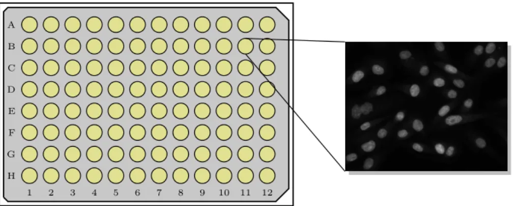
1.1 The basis of a systematic high content screen. A microplate
from which is registerd a fluorescence (single-channel)
mi-croscopy image highlighting the nuclei of a cell population. . 20
1.2 A conventional high content analysis follows four ordered stages.
Each stage may be accomplished by a variety of algorithms, and some stages may be omitted in certain pipelines, or
sub-sumed to a common framework.. . . 23
1.3 Comparison of cells sampled from negative control wells
con-taining (a) TNBC cell line MDA231 and (b) TNBC cell line MDA468. Cell nuclei appear in blue, cell microtubules appear
in red. . . 25
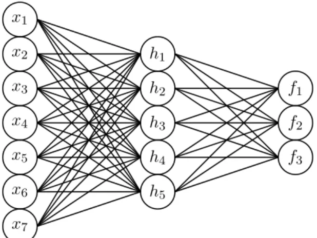
2.1 Fully-connected neural network with 7 input neurons, a single
hidden layer with 5 neurons, and an output layer with 3 neurons. 33
2.2 Convolution operation consisting of (from left to right) an
input image, convolutional kernel, and convolved output im-age. The valid convolution results in the loss of the border pixels. Notice how the output represents the gradient image, obtained by setting the kernel to the finite difference between
vertically adjacent pixels. . . 35
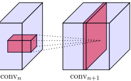
2.3 Each kernel of a convolutional layer (in red) performs a
con-volution as a tensor-product at each spatial location of an incoming tensor, to produce a single activation map
(chan-nel) in the output tensor. . . 37
2.4 Object detections made by pre-trained R-CNN available in
PyTorch (Paszke et al. [2017]). The image was taken in the
Kyoto Gogyo ramen restaurant in Kyoto. . . 40
2.5 Data augmentation can make modest but useful interpola-tions of the space surrounding real images. CIFAR-10 images marked by red circle; augmented images marked by blue cir-cle; black line represents natural image manifold. Upper aug-mentation based on conversion to grayscale (an element-wise weighted average of the RGB pixels) and rotation; the lower
on colour inversion and horizontal flipping. . . 43
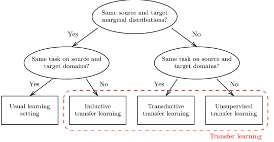
2.6 Positioning transfer learning with respect to the typical
learn-ing settlearn-ing. Categories of transfer learnlearn-ing differ either with
respect to the marginal distribution. Reproduced from https://en.wikipedia.org/wiki/Domain_adaptation 45
2.7 Overlapping domains (a) and divergent domains separated by
a linear decision boundary (b). . . 47
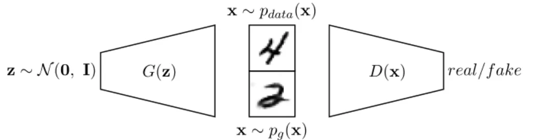
2.8 A GAN trains a generator network G to fool a discriminator
network D in emitting counterfeit images x ∼ pg(x) by
trans-forming noise input z. In order to do so, G must (implicitly)
learn the data-generating distribution, pdata.. . . 49
3.1 Fluorescence image of MDA231 cells. DAPI highlighting the
nuclei in blue, cyanine 5 highlighting the microtubules in red, and cyanine 3 highlighting the double-strand breaks as white
spots on the cell nuclei. . . 60
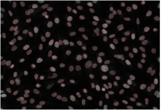
3.2 Nuclei segmentation on the DAPI channel, with segmentation
contours indicated by red bands. . . 63
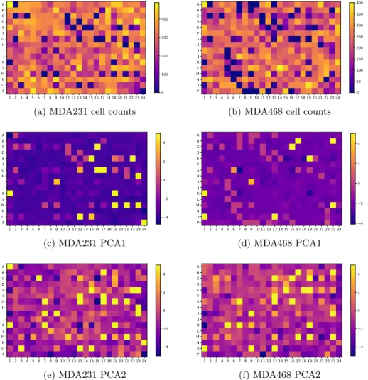
3.3 Searching for spatial biases: comparison of cell counts (a), (b);
comparison of first principal component of morphological pro-files (c), (d); comparison of second principal component (e), (f), arranged according to the plate map of the microplate. Left column (a), (c), and (e) pertain to cell line MDA231;
right column (b), (d), (f) to cell line MDA468. . . 67
3.4 Viability comparison between cell lines for a variety of drugs
and negative controls. The neutral DMSO and untreated
wells strongly overlap, while showing considerable variation in both cell lines. Viability correlates well between cell lines
with Pearson correlation coefficient ρ = 0.6556 . . . 68
3.5 Comparison of viability by drug mechanism of action. One
may observe differential effects by cell line: (a), (b) show dif-ferential effects on viability; (c) shows no clear divergence from the control cluster; (d), (e), (f) show a range of
LIST OF FIGURES 9
3.6 Drug perturbations inducing significant changes to DSB
dis-tribution (measured by spot density) on cell line MDA231 at
p = 0.01 with multiple testing correction, ordered by median
spot density. Sample of cells perturbed with significant drug PKC-412 (b), DSBs visible as green spots above nucleus. A bimodal distribution is seen on the DAPI channel revealing a growth of mean intensity post DNA replication (c). An Otsu threshold (red vertical line) can be used to stratify the cell population, further revealing distributional differences in
DSB rates. . . 71
3.7 Morphological profiles of 12 TNBC cell lines with 8 replicates
apiece, based on 7 biologically meaningful classes, derived from manual annotation. One observes the phenotypic
simi-larity between cell line families. . . 74
3.8 UMAP projection from feature space of sample cells from four
TNBC cell lines (selected among 12) in a wild type screen. On the right we show a fixed-size (128 × 128px) crop centered
on an indicative cell from each cell line. . . 75
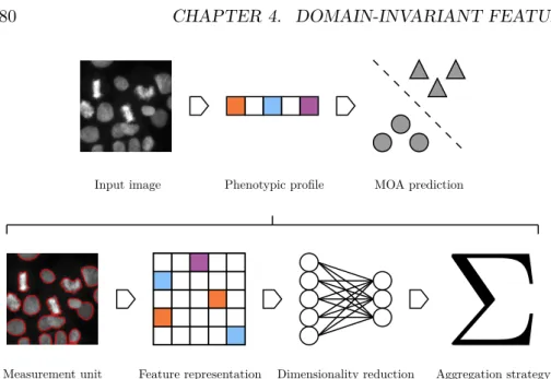
4.1 MOA prediction is performed on an image via a phenotypic
profile. The development of such a profile spans four ordered stages. Each stage may be accomplished by a variety of al-gorithms, the combination of which define a unique pipeline. Some stages may be omitted in certain pipelines, or subsumed
to a common framework.. . . 80
4.2 Example of how phenotypic profiles may cluster with a
hier-archical model and Ward linkage for 40 drugs in 8 mechanism of action classes (including negative control)s from our drug screen data set. Heat map colour indicates distance between profiles, and dendrogram leaf colours indicate mechanism of
action class. . . 81
4.3 Multitask autoencoders used for dimensionality reduction over
multi-cell-line data. Clockwise from top left: vanilla coder, multitask autoencoder, and domain-adversarial autoen-coder. Colouring indicates separate treatment of each domain
(cell line). . . 87
4.4 t-SNE embeddings of encodings from autoencoder (left) and
domain-adversarial autoencoder (right), with cell lines distin-guished by colour, and mean silhouette scores of 0.11 and 0.01
4.5 MDS embedding of drug effect profiles for MDA231 and MDA468 cell lines with DMSO centroid centered on origin. Detection of differential drug effects between cell lines with examples for each category below (MDA231 top, MDA468 bottom). From left to right: no drug effect in either cell line (negative control); drug effect in MDA231 cell line only; drug effect in MDA468 cell line only; similar drug effects in both cell lines; differentiated drug effects in both cell lines. Shown are
example images, blue: DAPI, red: microtubules, green: DSB. 92
4.6 t-SNE embeddings of encodings from handcrafted features
(left), autoencoder (center) and domain-adversarial autoen-coder (right), with cell lines distinguished by colour. Respec-tive silhouette scores of 0.22 and 0.14 and −0.02 confirm the
reduced divergence in the adapted domains. . . 94
5.1 Aligned image channel crops (200 × 200px) marking living
Raji cells in mCherry (left), dead cells in GFP (center), and
phase contrast (right). . . 104
5.2 Tracking apoptosis of a Raji cell. GFP signal accumulates as
a cell undergoes morphological changes (a)-(f). . . 105
5.3 Raji cell population over time. Proliferation generates cell
clusters. . . 106
5.4 CAR-T cells (devoid of fluorescence) attack Raji B cells by
latching onto Raji cell surface antigens and delivering cyto-toxic chemicals. The induced lysis of the target Raji cells
yields growing clusters of cellular matter. . . 106
5.5 Comparison of average GFP (left) and mCherry (right)
fluo-rescence measured across different fields of view at 24 hour in-tervals. One may observe the quenching effect of fluorescence
over time, which occurs most rapidly in the first increment. . 107
5.6 Pearson correlation coefficients for outputs of three
fluores-cent labelers, for both mCherry and GFP fluorescence
pre-diction, measured over 80 test images. . . 111
5.7 Full fluorescence for indicative (512 × 512px) crop from an
Raji-only experiment. Columns distinguish fluorescent
la-beler predictions (left) and ground truth (right); rows dis-tinguish times an early frame (t = 0) (top) and a later one
(t = 48) (bottom). . . . 113
5.8 Full fluorescence for indicative (512 × 512px) crop from a
CAR-T experiment. Columns distinguish fluorescent labeler predictions (left) and ground truth (right); rows distinguish times an early frame (t = 0) (top) and a later one (t = 40)
LIST OF FIGURES 11
5.9 Fluorescent labeler outputs produce dense clouds of mCherry
fluorescence for two manually selected phase contrast inputs.
These outputs may be difficult to disambiguate.. . . 116
5.10 Pipeline for automatic construction of ground truth for train-ing object detection system. Basic image processtrain-ing steps
indicated in blue, image inputs indicated in red.. . . 118
5.11 Living and dead Raji cells revealed as distinct modes of a bimodal distribution on mean GFP fluorescence intensity per
connected component of cell segmentation output. . . 119
5.12 Samples of living Raji cells (top), dead cells (middle), back-ground (bottom) annotated with bounding boxes.
Fluores-cence is included for clarity only and is not used in training. . 120
5.13 Pipeline for training a deployment of a fully convolutional classifier. Training may occur on fixed-sized input (24×24)px,
but convolutions permit variable-sized inference. . . 121
5.14 The processing of a test image: phase contrast input image (a); raw model bounding box predictions (b); non-maximum suppression post-processing (c); finally, for comparison, the
corresponding full fluorescence image (d). . . 122
5.15 Population curves for manually-annotated test set A (a) and
test set B (b), compared with detection system outputs. . . . 126
5.16 Comparing cell quantification strategies by accumulation of cell types over time in four well replicates, aggregating over fields of view. The labeling series are normalised to have the
same mean as the detection series. . . 128
6.1 Example cell-centered 24 × 24px crops from the ground truth
training set. . . 130
6.2 Sample 24 × 24px crops from a fully-connected GAN. . . 131
6.3 Sample 24 × 24px crops from a DCGAN. One may notice the
generator has learned to synthesise convincing peripheral cells.132
6.4 Comparison of cells generated with DCGAN (left-most
col-umn) against 9 nearest neighbours from training set. . . 132
6.5 Sample 24 × 24px crops from a conditional DCGAN. The top
row are crops produced by conditioning for living Raji cells; the bottom are crops produced by conditioning for dead Raji
cells. . . 133
6.6 A neural algorithm of artistic style uses a pretrained CNN to
combine properties from a style source image (a) and a con-tent source image (b) to synthesise a new image combining
their characteristics (c). Example taken from https://github.com/jcboyd/vgg-fun . . . 135
6.7 Example of Voronoi tessellation with six sites (blue points) and corresponding regions (yellow lines) (generated in scipy
(Virtanen et al. [2020]) (a). Neighbouring cells exhibit a
tes-sellating effect at the border (b). A conditional dilation al-gorithm can model this bordering effect when it comes to
synthesising content images for style transfer. . . 137
6.8 An example of generating a cell content image by first
allocat-ing sites with AllocateSites (a) (site intensity represents radius, dilated for visibility), with radii drawn from Equation 6.5; running the ConditionalDilation algorithm to obtain labeled regions as in Equation 6.7 (b); and extracting the
contours with Equation 6.8 (c). . . 140
6.9 An application of a neural algorithm of artistic style to phase
contrast images of CAR-T cells (a) and a style source image (b) to synthesise a new image combining their characteristics
in a “simulated” image (c). . . 140
6.10 More cells, more problems. The style transfer algorithm fails when the content image does not offer adequate “scaffolding”
for the target texture patterns. . . 141
6.11 Examples of CycleGAN generated images. Columns organ-ised with content specification input image X (left), G(X) generated image (center) and reconstruction F (G(X)) (right). The number of cells are increased over the rows: 25, 50, 100,
and 150. . . 144
6.12 Comparison of outcomes of Faster R-CNN on a test image when a) fine-tuned on a weakly supervised dataset and b)
fine-tuned on synthetic images. . . 145
6.13 Conceptualisation of an extension to adversarial image-to-image translation networks with a region of interest
discrim-inator Droi. The Droi relies on a library of real crops to
compare to cells synthesised by G in the prescribed regions
of the content image. . . 148
A.1 Confusion matrix for a random forest classifier classifying cells
from 12 TNBC cell lines.. . . 157
A.2 Plate map of perturbations used for drug screen. Empty cells
indicate empty wells. DMSO denotes negative controls. . . . 158
A.3 MDS plots of each category of drug effect. The distances between the profiles are plotted as a line, as well as the
re-spective distances to the centroid (origin). . . 159
A.4 A living Raji cell (a) is attacked by a CAR-T cell (b) and
later dies (c). . . 160
A.5 Tracking the apoptosis of a Raji cell. Counterpart to Figure 5.2. . . 160
LIST OF FIGURES 13
A.6 Blob detection results. Left column shows ground truth,
right column shows pix2pix prediction. With respect to the ground truth: true positives: 31; false positives: 9; and false
negatives: 11. . . 161
A.7 An illustration of the automatic ground truth generation
im-age processing pipeline. The first row are the imim-age inputs. . 162
C.1 Examples of spots (red) on cell nuclei detected with diameter
openings on the Cy3 channel (grey). . . 174
C.2 Granulometry and spot density readouts show high
correla-tion on average over all wells. . . 175
C.3 Distribution of cell total intensities on the DAPI channel for MDA231 cell line (a). The bimodal distribution is a
conse-quence of the growth sustained between the G1(black) and G2
(red) phases of the cell cycle. A suitable threshold of DAPI intensity significant divergence in the DSB distributions of
the respective groups on the Cy3 channel (b). . . 176
C.4 Causal diagram including selection bias: P is the perturba-tion; D is the distribution of double-strand breaks and; A is the frequency of apoptosis. Conditioning (represented as a square) on the common effect of treatment P and outcome D
creates a selection bias. . . 177
C.5 Causal diagram showing effect modification of cell cycle phase:
G is cell cycle phase; P is the perturbation, and D is the DNA
damage. . . 178
D.1 Examples of spots (red) on cell nuclei detected with diameter
openings on the Cy3 channel (grey). . . 182
D.2 From left to right: canvas input, activation map after Max-Pooling layer, activation map after RoIAlign layer (reduced
to single bounding box). . . 183
D.3 Prediction of 16 digits over canvas, performed in a single
for-ward pass. . . 184
D.4 Encodings of class and localisation specificiation (left and cen-ter) and corresponding train image for training a conditional
GAN with RoI discriminator. . . 185
D.5 With the same specification of object localisation and class, a ground truth image (a), a synthetic image from a plain pix2pix system (b) and synthetic image from our pix2pix
List of Tables
2.1 Single-model test errors on ImageNet for five groundbreaking
CNNs. Note AlexNet was evaluated on the ILSVRC 2012 dataset, the others on ILSVRC 2014. Human performance
has been estimated to be 5% Top-5 error (Karpathy [2014]). . 39
3.1 The drug screen pilot data, consisting of two cell lines on
separate 384-well plates, with four fields per well. Four fluo-rescence channels are captured, under four acquisition modes. The full data set of 49152 images is the outer product of each
of the table fields. . . 59
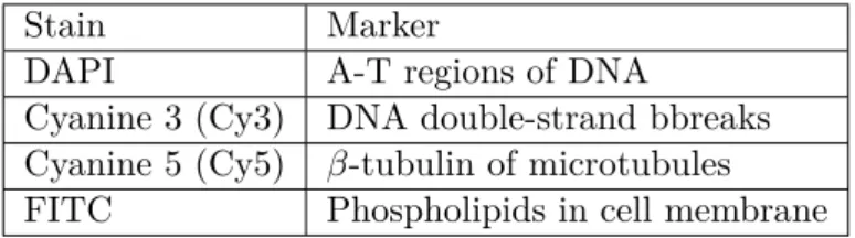
3.2 The stains used in the fluorescence microscopy of the screen
and their corresponding biological markers. . . 59
3.3 The wild type screen data, consisting of 12 cell lines evenly
distributed over a 96-well plate (ordered by column). Four fluorescence channels are captured as in the drug screen,
al-beit with FITC replaced by rhodamine in the final four rows. 61
3.4 TNBC cell lines and negative control MCF-10A properties
referenced from Chavez et al. [2010]. Drug screen cell lines
indicated in bold. 1Site: NB, normal breast; PE, pleural
effusion; PT, primary tumour. 2Pathology: AC,
adenocarci-noma; IDC, infiltrating ductal carciadenocarci-noma; IMC, infiltrating
medullary carcinoma. . . 62
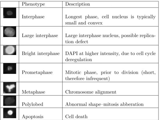
3.5 Morphological classes manually annotated on wild type screen
data to create a ground truth for training cell classifier. . . . 73
4.1 Comparison of dimensionality reduction approaches against
unreduced baseline for cell lines treated separately. We show mean and standard deviation of accuracies over 60 runs with
(∗) indicating significant results at the p = 0.05 level; (∗∗) at
the p = 0.01 level. . . . 89
4.2 MOA prediction on multiple cell lines (pooled) with
autoen-coders trained on handcrafted features. From top to
bot-tom: vanilla autoencoders (baseline), multitask autoencoders and domain-adversarial autoencoders. We compare with the
vanilla autoencoder (top row) ((∗∗) : p < 0.01) . . . 90
4.3 MOA prediction on multiple cell lines (pooled) with
convo-lutional autoencoders. From top to bottom: vanilla
con-volutional autoencoders (baseline), multitask concon-volutional autoencoders and domain-adversarial convolutional coders. We compare with the vanilla convolutional
autoen-coder (top row) ((∗∗) : p < 0.01). . . . 91
5.1 Characteristics of CAR-T experiments studied. Row A
stud-ies RAJI cells in isolation; row B studstud-ies cocultured Raji and
CAR-T cells. . . 103
5.2 Specification of the network architecture. We distinguish
three multitask outputs: Outputo, the probability of object
presence; Outputc, the probability of class c given an object;
and Outputb, the tuple of object width and height. . . 120
5.3 Detection performance test set A, stratified by object class.
Best results in bold. . . 124
5.4 Detection performance on test set B, stratified by object class.
Best results in bold. . . 125
5.5 Correlations between object detection and fluorescence
pre-diction time series for alive and dead Raji cells in four
exper-imental replicates. . . 127
C.1 Number of hits (out of 168) for each DSB quantifier on the
MDA231 cell line. Significance at the 0.01 level with the
Chapter 1
Introduction
Summary: Computational phenotyping is an emergent set of technologies for systematically studying the role of the genome in eliciting phenotypes, the observable characteristics of an organism and its subsystems. In partic-ular, cell-based assays screen panels of small compound drugs or otherwise modulations of gene expression, and quantify the effects on phenotypic char-acteristics ranging from viability to cell morphology. High content screen-ing extends the methodologies of cell-based screens to a high content read-out based on images, in particular the multiplexed channels of fluorescence microscopy. Screens based on multiple cell lines are apt to differentiating phenotypes across different subtypes of a disease, representing the molecu-lar heterogeneity concerned in the design of precision medicine therapies. These richer biological models underpin a more targeted approach for treat-ing deadly diseases such as cancer. An ongotreat-ing challenge for high content screening is therefore the synthesis of the heterogeneous readouts in multi-cell-line screens. Concurrently, deep learning is the established state-of-the-art in image analysis and computer vision applications. However, its role in high content screening is only beginning to be realised. This dissertation spans two problem settings in the high content analysis of cancer cell lines. The contributions are the following: (i) a demonstration of the potential for deep learning and generative models in high content screening; (ii) a deep learning-based solution to the problem of heterogeneity in a multi-cell-line drug screen; and (iii) novel applications of deep image-to-image translation models as an alternative to the expensive fluorescence microscopy currently required for high content screening.
Résumé: Le phénotypage computationnel est un ensemble de technologies émergentes permettant d’étudier systématiquement le rôle du génome dans l’obtention de phénotypes, les caractéristiques observables d’un organisme et de ses sous-systèmes. En particulier, les essais cellulaires permettent
de cribler des panels de petites molécules ou de moduler l’expression des gènes, et de quantifier les effets sur les caractéristiques phénotypiques al-lant de la viabilité à la morphologie cellulaire. Le criblage à haut contenu étend les méthodologies des criblages cellulaires à une lecture à haut con-tenu basée sur des images, en particulier les canaux multiplexés de la micro-scopie à fluorescence. Les cribles basés sur de multiples lignées cellulaires sont aptes à différencier les phénotypes de différents sous-types d’une mal-adie, représentant l’hétérogénéité moléculaire concernée dans la conception de thérapies médicales de précision. Ces modèles biologiques plus riches sous-tendent une approche plus ciblée pour le traitement de maladies mortelles telles que le cancer. Un défi permanent pour le criblage à haut contenu est donc la synthèse des lectures hétérogènes dans les cribles à multiples lignées cellulaires. Parallèlement, l’état de l’art établi en matière d’applications d’analyse d’images et de vision par ordinateur est l’apprentissage profond. Cependant, son rôle dans le criblage à haut contenu ne fait que commencer à être réalisé. Cette thèse aborde deux problématiques de l’analyse à haut contenu des lignées cellulaires cancéreuses. Les contributions sont les suiv-antes : (i) une démonstration du potentiel d’apprentissage profond et de modèles générateurs dans le criblage à haut contenu ; (ii) une solution basée sur l’apprentissage profond au problème de l’hétérogénéité dans un criblage de médicaments sur plusieurs lignées cellulaires ; et (iii) de nouvelles appli-cations de modèles de traduction d’image à image comme alternative à la microscopie à fluorescence coûteuse actuellement nécessaire pour le criblage à haut contenu.
1.1
Computational phenotyping
The success of the Human Genome Project (Lander et al.[2001]) in mapping the totality of human genes has inspired similar efforts for the enumeration of biological phenotypes. One useful relation views a phenotype as, in con-junction with environmental factors, the manifestation of the genetic code. Natural selection has been said to operate in the “P-space” of all possible phenotypes, with selection propagating to the “G-space” of all possible geno-types. Hence, phenetic information bears directly on important biological questions regarding disease and mortality (Houle et al.[2010]).
Unlike a genotype, which is constrained to the configuration of a fixed num-ber of genes, an organism’s phenotype spans the space of its observable characteristics. This notion is somewhat problematic, as what is observable has broadened in time with advancements in technology. As a result, an organism’s phenotype today may span its molecular, cellular, tissular, mor-phological, and behavioural traits, none of which are moreover necessarily fixed in time. For this reason, it is often convenient to refer to a tractable
1.1. COMPUTATIONAL PHENOTYPING 19 subset of an organism’s phenotype, for example that pertaining to an or-ganismal subsystem, such as the properties of its cells. As a result, the term phenotype and the related phenome are in practice want of semantic hygiene
(Mahner and Kary [1997]).
Phenomics, by analogy to genomics, refers to the study of high-dimensional readouts across the full spectrum of an organism’s phenotype (Houle et al.
[2010]). The interest in phenomics coincides with the rise of bioimage in-formatics (Myers [2012]). Bioimages, deriving from the various forms of microscopy, contain rich information on the morphological aspects of cells, cell populations in culture or tissue, and complete organisms, that is lost in other biological readouts. Bioimages in time-lapse can additionally reveal behaviour and track phenotypic changes in motion. Thus, bioimages are a favourable medium for phenotypic information.
1.1.1 High content screening
High content screening (HCS) is a methodology for the systematic discovery of phenotypes from image data in cellular assays (Haney[2008]). HCS may be viewed as extending the methodology of high throughput screening (HTS) to the medium of images. HTS is an experimental setup to test many experimental conditions in a systematic way, typically with a very simple readout, for example cell viability or a univariate measure of cytotoxicity. HCS performs such screens with a more complex and informative readout by leveraging, in particular, multiple channels of fluorescence microscopy. HCS thus increases the “content” of the readout to a large number of features (perhaps hundreds), while maintaining the throughput. HCS can be used for fundamental biological research, where gene expression can be modulated via techniques such as RNA interference, or otherwise knocked out entirely, inducing phenotypic effects in cultured cells. HCS has been instrumental in deciphering the molecular basis of a number of diverse biological processes, such as cell division (Neumann et al. [2010]), protein secretion (Simpson
et al. [2012]), and endocytosis Collinet et al. [2010]. HCS has also been
used to systematically screen for the localisation of biomolecules inside cells
Boland et al.[1998]).
HCS also plays a role in the early “hit-to-lead” stages of the drug discov-ery process (Haney et al.[2006],Pepperkok and Ellenberg [2006a]). In this case, a cell line population is exposed to small molecule drug compounds. Thus, the cell line is the model for a disease, and the screening process aims to identify the drugs that are active thereupon. For instance, one may be interested in identifying drugs that specifically kill cancer cells. HCS comple-ments other techniques for drug identification such as biochemical assays. For instance, Swinney and Anthony [2011] differentiate target-based and
H 1 G F E D C B A 2 3 4 5 6 7 8 9 10 11 12
Figure 1.1: The basis of a systematic high content screen. A microplate from which is registerd a fluorescence (single-channel) microscopy image highlighting the nuclei of a cell population.
phenotypic screens. The study looks at 257 drugs published between 1999 and 2008. Despite the preeminence of target-based approaches, they find the most common mode of first-in-class drug discovery is phenotypic screen-ing. This is most true of infectious and central nervous system diseases. Cancer treatments are most frequently discovered by biologics1, which also predominate for diseases of the immune system. Target-based approaches succeed for the discovery of half of all follower drugs.
1.1.2 The elements of high content screening
In order to perform experiments in high throughput, HCS relies to a signifi-cant extent on experimental automatisation. Experiments are conducted in wells arranged in a grid structure on a microtiter plate2 as depicted in Fig-ure1.1. The wells are seeded to confluence3 with cells of a chosen cell line. Within each well, a different perturbation experiment is conducted. In all bi-ological experiments it is important to rely on proper controls against which the tested perturbations are compared. Screens compare populations of neg-ative controls (unperturbed) with others exposed to perturbation. Positive controls take the form of perturbations with a known effect, such as small molecule cytotoxicity in a drug screen. Some number of images correspond-ing to non-overlappcorrespond-ing fields of view (henceforth fields) are taken from each well, typically producing from hundreds to thousands of unique images per plate. The following briefly describes the key elements of a screen.
1Biologics are genetically-engineered proteins that target the immune system.
2
Microtiter plates (hereafter plates) are small (usually polystyrene) trays divided into a rectangular grid of wells functioning as individual test tubes.
3
1.1. COMPUTATIONAL PHENOTYPING 21 Cell lines
The object of analysis of an HCS assay is an immortalised cell line (hereafter referred to as a cell line), which consists in a population of cells, sustained by division without senescence. As a result, a cell line continues replicating indefinitely from a common ancestor. Cell lines are the biological model acting as a representation of the disease. The first and most well-known cell line generated is the HeLa cell line (Scherer et al. [1953]). Since HeLa, many cell lines have been developed. Cell lines are useful biological models due to their longevity in cell culture, and are used extensively in biomedi-cal research, for example in assessing the cytotoxicity of a drug treatment. However, their accuracy as biological models can be compromised by their inherent mutations, and the effects of repeated passages, cloning, and bio-chemical contaminants can lead to significant genetic drift from their in vivo ancestors (Marx [2014]). Despite these limitations, cell lines remain the most widely used model system in screening, and many scientific and pharmacological discoveries have been made from screens on cell lines.
Microscopy and fluorescence
In high content screening, imaging data derives from one or another of the many types of optical microscopy. A broad range of techniques for perform-ing microscopy exist, each leveragperform-ing the principles of optics in different ways, and the technique will be tailored to the experimental objectives. Bright-field microscopy passes visible light through a sample, producing a picture in which light is attenuated according to the varying densities of the imaged specimen. Phase contrast is a more sophisticated variant of transmitted light microscopy, measuring the phase shift of the visible light traveling through the specimen, producing an image with a greater degree of contrast.
Fundamental to high content screening is fluorescence microscopy, which uses a laser to excite fluorescent molecules in organic matter. These molecules are known as fluorophores and emit light at a unique wavelength (think colour) upon excitation by a laser. As such, localised fluorophores can be utilised to highlight key cellular regions. The predominant technique used in HCS is immuno-fluorescence, which relies on fluorescently-labeled anti-bodies. Other widely used techniques include labeling of live samples, stable expression, or fluorescence in situ hybridisation. In most screening applica-tions, the nuclei are stained with one of these techniques, allowing for the subsequent identification of individual cells. The other fluorescent markers are selected in accordance with the research questions, for example, mi-crotubules, Golgi apparatus, or plasma membrane. Thus, the fluorescence
markers of a screen, responding to distinct wavelengths of light, yield a set of multiplexed images painting a composite picture of the cell in its key sub-cellular structures. Image analysis can then be used to extract the high content readouts of the screen.
Project workflow
A typical HTS project workflow commences with a pilot screen that vali-dates the pipeline from experimental protocol through to image analysis (see
Terjung et al.[2010]). This is followed by a large scale screen, increasing the
number of perturbations tested. It is here that candidate hits (drug pertur-bations registering a significant effect) are identified by automatic analysis (see the following Section1.1.3). Finally, candidate hits are carried forward to secondary screens and are studied in greater detail.
1.1.3 High content analysis
With a large image dataset in hand (Section1.1.2), so begins the automated image analysis, or high content analysis. Each image depicts a population of cells subject to perturbation or else representing a control case. The aim is to attribute a phenotype to the population in terms of a specific measurement or vector of measurements. Analysis of the pixel values across the various fluorescent channels yields a set of features or readouts. Cell phenotypes are compiled through feature extraction of each measured unit of the image. The distribution of perturbed readouts can be compared to control cases in a statistical framework so as to establish screen hits. In order of complexity, the readouts may be categorised according to the following:
I Univariate: In the ideal case, biological functions may be quantita-tively described by a single feature. For example, the nuclear area might increase dramatically under certain treatments. Thus, it would be sufficient to measure the corresponding feature (nuclear size) and statistically analyse its distribution under the different experimental conditions. Such a scenario would likely be easier to explain in biolog-ical terms.
II Multivariate: A more complex case arises when one analyses differ-ent phenotypic descriptors (biologically meaningful features) and their interdependencies. Then one would contend with the multi-variate dis-tribution of these features, and the analysis would be necessarily more sophisticated.
III Machine learning: In a final case, phenotypes might not be dis-cernible in such basic terms, and would rather require the tools of
1.1. COMPUTATIONAL PHENOTYPING 23
Σ
Measurement unit Feature representation Dimensionality reduction Aggregation strategy
Figure 1.2: A conventional high content analysis follows four ordered stages. Each stage may be accomplished by a variety of algorithms, and some stages may be omitted in certain pipelines, or subsumed to a common framework.
statistical learning to elucidate more subtle patterns in the cell popu-lation. In this case, one would rather extract a large number of features without clear biological meaning. Learning can then be supervised or unsupervised. In the supervised case, the biological meaning could be injected (by the analyst) through use of biologically meaningful classes.
These readouts may be taken at various scales. However a logical (and in-deed, conventional) starting point is at the level of individual cells (Perlman
et al. [2004], Adams et al. [2006]), entailing an initial segmentation of the
image. As a side note, it is for this reason that it is favourable to seed cells at a density that will minimise cell overlap. The seeding density must therefore be chosen according to the unique morphological properties of the cell line (Bray et al.[2016]). However, segmentation-free approaches directly analysing the full image (Orlov et al.[2008],Uhlmann et al.[2016]), or image segments, have proven successful, in particular through application of deep learning (Kraus et al.[2016]). The tradeoff is between a fine-grained anal-ysis at the cellular level, where careful consideration of cell structure and fluorescent colocalisation is a focus (Slack et al.[2008]), and a coarse analy-sis of the cell population, where population densities and dynamics can be measured. Attempts to benefit from both scales have been made (Godinez
et al. [2017]). After these early stages of image analysis, a screen dataset
is usually subject to a range of quality control procedures, which may use automatic techniques to detect artifacts such as image blur or saturation, or else detect outliers among cells that have been under- or over-segmented
(Caicedo et al. [2017]).
After these initial stages, particularly a type III analysis may proceed to-wards a phenotypic profiling of the cell population. Figure1.2 encapsulates a conventional approach to profiling. Dimensionality reduction is used vari-ously to eliminate redundant features, as well as to compress the data into its
essential components (for example, the set of principal components derived over the population of cell feature vectors). Here, the options abound and the choice of method is determined by the analytical objectives. A simple, motivating example is the case of counting classes of cells in a population. Here, a classifier (such as in Neumann et al. [2010]), performs the role of dimensionality reduction: the classifier maps the feature vector of each cell to a scalar or one-hot encoding representing cell class,
f : x → {0, 1}K, (1.1)
for K classes of cells. The population phenotype is then summarised in p ∈ RK, obtained by aggregation as a simple summation or average, giving the number or proportion of cells per cell class respectively,
p = 1 N N X i=1 f (xi), (1.2)
for the N cells in the population.
1.2
Challenges for high content analysis
High content analysis offers many interesting research directions. Those most relevant to this dissertation are described in the following.
1.2.1 Multi-cell-line data
As mentioned before, the use of a single cell line limits HCS as a drug screening approach. Diseases, in particular, cancer, are often heterogeneous on a molecular level. This translates therapeutically to scenarios in which a treatment effective against one molecular subtype is ineffective against (or even promotes genetic instability in) another subtype. Hence, a single cell line introduces a bias towards a particular disease subtype. This motivates the validation of discoveries against multiple cell lines, representing different subtypes of the same disease. A screen based on multiple cell lines, repre-senting multiple disease subtypes, can help in formulating hypotheses on, for example, the mechanism of resistance to disease. This is furthermore a step in the direction of the emerging paradigm of precision medicine (Ashley
[2016]), where machine learning will play a decisive role (see, for example,
Krittanawong et al. [2017]). Genomics has led the way so far, but other
data sources including images are expected to become increasingly part of the picture Hulsen et al. [2019]. This has motivated a large consortium of
1.2. CHALLENGES FOR HIGH CONTENT ANALYSIS 25
(a) MDA231 (b) MDA468
Figure 1.3: Comparison of cells sampled from negative control wells con-taining (a) TNBC cell line MDA231 and (b) TNBC cell line MDA468. Cell nuclei appear in blue, cell microtubules appear in red.
research groups to propose multi-cell-line drug screens, and to build models capable of predicting the efficiency of a drug from the transcriptomic and genetic data of the cell-line (Costello et al.[2014]). However, the success of these approaches has been rather modest. One of the reasons for this was the measurement of drug efficiency, that reduced the drug effect to a single number. Drug effect similarities cannot be reasonably calculated from such data. One therefore stands to gain from studying multi-cell-line drug effects rather in high content phenotypic profiles.
A key use case for HCS in drug screens is the related problem of target prediction, that is, the prediction of the pathway or protein whose function is altered by the drug. This invokes a classification task on the image data, namely to determine what mechanism of action (MOA) is responsible for inducing the effects visible in the perturbed populations, often judged with reference to the control populations. Screening several cell lines with dif-ferent genetic and transcriptomic profiles allows one to test more pathways (as not all genes are expressed in all cell lines) and, in so doing, to get a richer description of the MOA of the drug. Quantifying drug effects with re-spect to multiple cell lines allows to distinguish cell-line-specific drug effects from unilateral effects. A multi-cell-line screen, in which several cell lines representative of a common disease are subjected to the same set of per-turbations, is therefore well motivated. However, such a screen creates the challenge of a data heterogeneity. For example, TNBC cell lines MDA231 and MDA468 manifest different morphologies in their unperturbed state. Figure 1.3 shows samples of cells from these two cell lines, taken from
mi-croplate wells containing negative control substance dimethyl sulfoxide, with the cells imaged by the same set of fluorescent markers. One observes clear differences in these archetypal morphologies, with MDA231 cells exhibiting elongated nuclear and cellular shapes, compared to the isotropic MDA468 cells. This has additional, second-order effects such as the degree of geomet-ric tessellation between groups of cells. Note that in single-cell-line data, population phenotypes aggregated from the single cell constituents already abandon distributional information (Altschuler and Wu [2010]), as multi-modal populations are often reduced to their unrepresentative centroids. This problem is potentially exacerbated in multi-cell-line data and remains a challenge. Combining multi-cell-line image data has so far been unat-tended, with a handful of exceptions such asRose et al.[2018] andWarchal
et al.[2016].
1.2.2 The emergent role of deep learning in high content
screening
Deep learning is touted as a panacea for computer vision problems, and high content data ought not to be an exception. In applications of deep learning, a neural network may perform several of the HCA stages (Figure 1.2) si-multaneously, as neural networks naturally incorporate elements of feature extraction and dimensionality reduction (Sommer et al.[2017] is a good ex-ample). However, the successful deployment of deep neural networks relies crucially on vast volumes of data to enable effective generalisation. Large annotated datasets such as ImageNet (Russakovsky et al. [2015]) were one of a few key preconditions that fostered the rise of deep learning for object classification in 2012, and extensions of deep learning to other problem do-mains were likewise accompanied by the curation of large, special-purpose datasets, for example Lin et al. [2014] for object detection. However, an-notated data for supervised training is expensive, requiring manual effort, often by domain experts. ImageNet leverages online crowdsourcing plat-forms (quality is ensured by the consensus of multiple annotators). This is a bottleneck for all deep learning research, and therefore extends to compu-tational phenotyping. The Broad Institute benchmark collection (BBBC) datasets (Ljosa et al.[2012] and, specifically,Caie et al.[2010]) have become a sort of benchmark for developing drug response phenotyping algorithms (for example, Kraus et al. [2016] or Kandaswamy et al. [2016]). However, while benchmark data sets are of course useful and have had an enormous impact on the field, we still face the problem that for new imaging projects, we do not have enough data to train neural networks. This relates to the fact that bio-images tend to be extremely variable between different projects: the visual aspect is heavily influenced by the choice of markers and the mode of microscopy. Indeed, by selecting different markers, one is effectively
look-1.2. CHALLENGES FOR HIGH CONTENT ANALYSIS 27 ing at different objects. For this reason, it seems unlikely that large scale datasets will definitively solve the problem of annotated data, except for the most widely used markers and imaging modalities.
Nevertheless, in recent years, a significant trend in deep learning research has been on making better use of available data. After all, even if annotated data is hard to come by, unlabeled or weakly labeled is available in abundance. For example,Mahajan et al.[2018] used 3.5 billion social media images “weakly annotated” with hashtags to pretrain a state-of-the-art system for object classification. Indeed, notable applications of deep learning in HCS thus far have relied on weakly supervised learning (Kraus et al.[2016],Godinez et al.
[2017]). Elsewhere, contrastive learning (for example, Chen et al. [2020]) may yet revolutionise the training of deep learning systems, achieving parity with state-of-the-art systems with the efficient use of only a small fraction of the data.
A recent trend in bioimage analysis has been the prediction of one mode of microscopy from another. Microscopes with the capacity of registering mul-tiple modes of microscopy simultaneously (for example, transmitted light and fluorescence images) automatically create an image-to-image transla-tion dataset. Fluorescence labeling as a pixel-wise regression problem has been successfully demonstrated byChristiansen et al. [2018] andOunkomol
et al. [2018], where deep multi-task neural networks are furthermore
ca-pable of labeling multiple independent fluorescent channels simultaneously. Earlier, Sadanandan et al. [2017] used fluorescence to construct cell seg-mentation datasets automatically. These works have shown how one may exploit imaging protocols to bypass the manual annotation bottleneck for deep learning.
Generative models represent another trend in computer vision (Kingma and
Welling[2013], Goodfellow et al.[2014a], Oord et al. [2016]), modeling the
marginal distribution on data, allowing for data synthesis, in particular im-age synthesis, as well as unsupervised representation learning. Generative adversarial networks (GANs) (Goodfellow et al.[2014a]) are the most highly developed of deep generative models, and have already found use in high con-tent image data, for example inOsokin et al. [2017]. Elsewhere, generative models such as variational autoencoders (Kingma and Welling [2013]) have found use in phenotyping drug effects for MOA prediction. Image-to-image translation (see above) is also addressed by generative models capable of deep style transfer (Isola et al. [2017], Zhu et al. [2017]). Data synthesis is additionally a form of data augmentation, which in turn is an attempt to make more effective use of a scarce data supply. Moreover, it is one possible route towards the simulation of image data (see Ihle et al.[2019]). Unlike more standard deep learning models, however, generative models are more difficult to train, and may require creative and non-standard solutions.
Therefore, as much as the role of deep learning in high content analysis is not yet fully defined, the role of generative models is ever more so, and their application represents a fertile research direction.
1.3
Contributions
This dissertation encompasses work completed on two unique projects in high content analysis. At is likewise organised into two parts, each con-taining two chapters. The two parts can be read in any order, but they internally follow a progression of ideas that are intended to be read in order of appearance. Each chapter is oriented around a published paper, with the exception of the final chapter, which describes a work in progress. In addition, the optional Chapter 2 serves as an introduction to the basics of deep learning, with an emphasis on the models encountered throughout the dissertation.
Part I, comprising of Chapters 3 and 4 covers a high content drug screen of multiple TNBC cell lines. TNBC is a molecularly heterogeneous type of breast cancer with poor prognosis and limited treatment options. Its molecular heterogeneity makes finding treatments difficult, and a screen of multiple cell lines is therefore promising. Chapter3is introductory and aims to describe the workflows of high content screening and its modes of analysis, while following use cases from the drug screen, including a multivariate analysis on double strand break detection, published in the proceedings of ISBI 2018 (Boyd et al.[2018]) (included in AppendixC. It concludes with a use case of phenotypic profiling as a segue to Chapter4, which itself serves as a review of profiling methodologies, and develops a new profiling approach for multiple cell lines. The approach is to combine heterogeneous data from different cell lines using domain adaptation. Cells from the divergent cell line domains are mapped to a domain-invariant feature space by an adversarial neural network training strategy (Ajakan et al. [2014]). The chapter is an extended version of a paper published in the journal Bioinformatics (Boyd
et al.[2020a]). The dataset for this project is additionally released publicly
(Boyd et al. [2019a]) (it seems, the first of its kind), alongside an open
source code repository including worked, reproducible workflows4. In spite of the idealised workflow presented in Section 1.1.2, Part I is restricted to the pilot phase of a planned larger screen. Nevertheless, ample phenotypes are observed and on which to develop the new methods.
Part II, comprising of Chapters 5 and 6 covers chimeric antigen receptor T-cell (CAR-T) therapy experiments, which study the Raji cell line as a model for lymphoma. Though not strictly based on a screen, Part II uses
4
1.3. CONTRIBUTIONS 29 high content analysis and shares many characteristics with Part I. Chapter
5compares two approaches to utilising fluorescence microscopy as an auto-matic annotator of paired phase contrast microscopy. The second of the two approaches, based on a customised object detection system, was published in the proceedings of ISBI 2020 (Boyd et al. [2020b]). The datasets are again made public (Boyd et al. [2019b]), as well as source code and scripts for reproducible experiments5. A modified version of this paper is included inline in Chapter 5. Finally, the shortcomings of the two approaches are assessed in Chapter6, and a creative alternative solution is proposed, based on data augmentation via images synthesised with generative models. The final section of the chapter is intended as a prototype for a future publica-tion.
Not included in this dissertation are minor contributions made as a sec-ond author to a study on predicting residual cancer burden from TNBC histopathology images, published in the proceedings of ISBI 2019 (
Nay-lor et al. [2019]), and an as-of-yet unpublished paper on a new structured
dropout algorithm for regularising neural networks Khalfaoui et al.[2019].
5
Chapter 2
Deep learning
fundamentals
Summary: This dissertation makes extensive use of artificial neural net-works and deep learning. This chapter explores the basic properties of neural networks and shows how these ideas extend to the deep convolutional net-works key to modern image processing. It further briefly traces the history of the development of deep learning, and its extension into the various problem domains of computer vision.
Résumé: Cette thèse fait largement appel aux réseaux de neurones arti-ficiels et à l’apprentissage profond. Ce chapitre explore les propriétés de base des réseaux de neurones et montre comment ces idées s’étendent à la variété profonde et convolutionnelle des réseaux, clé du traitement moderne des images. Il retrace ensuite l’histoire du développement de l’apprentissage profond et de son extension dans les différents domaines de la vision par ordinateur.
2.1
The building blocks of artificial neural
net-works
An artificial neural network (henceforth neural network) is a collection of computational units known as neurons, organised into a sequence of layers. An input passes forward through a neural network, undergoing a series of transformations through combination with a set of weights in each layer. During a training procedure, the neural network is shown examples of input data paired with target outputs. After each round of training, the neural network adjusts its (randomly initialised) weights so as to make it a little
more likely to emit the target values given future appearances of the input data.
A simple neural network invokes one or more hidden layers between input and output, for example,
h(x) = σ(W(1)x + b(1)) (hidden layer)
f (x) = S(W(2)h + b(2)) (output layer) (2.1) for input vector x, first layer weights and biases matrix W(1) and vector b(1), and second layer weights and biases matrix W(2) and vector b(2). The
function σ is a non-linear activation function1and S is the softmax function at the output layer. The softmax is optional but often used for classification problems as it maps its inputs to categorical probabilities. In this case, the network is normally trained against a cross entropy loss function,
L =X i
− log(pyi), (2.2)
where pyi = f (xi)yi is the network output (probability) for the ith training
input xi, indexed at the (paired) ith target label yi. Equation2.2is a simpli-fication of the cross entropy formula for the case where the yiare “one-hot”, that is, all the probability mass is allocated to a single, “true” value. Note that neural networks can be trained for classification, regression, or unsu-pervised feature extraction, depending on the structure of the dataset. Each entails a different output layer and loss function for the network. Figure2.1
depicts an example of the simple neural network architecture in Equation
2.1.
The neural network framework gives freedom over the number of layers and the number of neurons in each layer. The more neurons, the more expressive the network, yet the more likely overfitting becomes2. We may extend to a multi-layer network simply by stacking the desired number of layers,
f (x) = S(W(M )σ(W(M −1)(· · · σ(W(1)x + b(1)) · · · ) + b(M −1)) + b(M )). (2.3)
1Historically, this was the logistic function, σ(x) = 1/(1 + exp {−x}), a continuous
approximation to the Heaviside step function (think on/off), however, in recent years, it has been superseded by the ramp function, more commonly known as the rectified linear unit, ReLU(x) = max(0, x), which provides various training benefits.
2It is rare to require more than three fully-connected layers, however, and exceeding
2.1. THE BUILDING BLOCKS OF ARTIFICIAL NEURAL NETWORKS33 x1 x2 x3 x4 x5 x6 x7 h1 h2 h3 h4 h5 f1 f2 f3
Figure 2.1: Fully-connected neural network with 7 input neurons, a single hidden layer with 5 neurons, and an output layer with 3 neurons.
Thus, the network layers are linear transformations interspersed with non-linear functions. When the inputs correlate positively with a vector of weights, the corresponding hidden layer neuron tends to become active via the non-linearity. In this way, each neuron of a hidden layer amounts to a feature detector for the prior layer. The hidden layer activations are then recombined in the next layer, and so on, allowing for ever more complex aggregations of features. This is the essence of deep learning. However, this tends not to work very well without certain inductive biases, (and, indeed, an amenable dataset) which we will encounter in Section2.2.
Despite their inherent non-linearity, and non-convexity, neural networks can be trained with standard gradient descent,
θt+1← θt− α · ∇θL, (2.4)
for the full set of model parameters θ and learning rate α. More sophis-ticated update rules than vanilla gradient descent exist such as RMSprop
(Tieleman and Hinton [2012]), and Adam (Kingma and Ba [2014]). These
methods improve over Equation 2.4 by adapting a learning rate for each parameter (rather than one-size-fits-all). Whatever the chosen method, the gradients are always computed using the backpropagation algorithm, which we examine presently.
2.1.1 Backpropagation
The procedure for computing the gradients at each iteration of gradient de-scent is called backpropagation. Backpropagation is an application of the
chain rule to the graphical structure of the neural network. The crucial for-mula for backpropagation, as presented inRumelhart et al.[1985] is,
∂L ∂xi =X j ∂L ∂yij ·∂yij ∂xi , (2.5)
that is, the gradient of neuron xi at a given layer l is the sum product of the gradients of the neurons of the following layer (l + 1) emanating from it yij and the gradient of the connections between them. From a practical standpoint, each layer l over which we perform backpropagation requires three computations:
1. ∂L
∂s(l), the gradient of the scores, s
(l) = W(l)x(l)+ b(l). Note this is a
“pseudo-layer” between the linear transformation and the activation. 2. ∂L
∂W(l), the gradient of the weights. These are recorded to ultimately
make the descent step (Equation2.4). 3. ∂L
∂x(l) =
∂L
∂σ(l−1), the gradient of the input (previous activation). This is
the error signal that is passed back to the layer below.
Let us first consider (1), the gradient of the scores. In general, we compute, ∂L ∂s(l) = ∂L ∂σ(l) · ∂σ(l) ∂s(l) where ∂L ∂σ(l) = ∂L
∂x(l+1), since the activation of the present
layer is the input to the following layer. The activation function σ is applied element-wise. Consequently, in the pseudo-layer between linear transform and activation, each neuron has a single connection. Therefore, with re-spect to Equation 2.5, the sum reduces to a single element per gradient giving, ∂L ∂s(l) = ∂L ∂σ1(l) · ∂σ(l)1 ∂s(l)1 .. . ∂L ∂σk(l) · ∂σ(l)k ∂s(l)k , (2.6)
where for sigmoid,∂σ
(l) i ∂s(l)i = ∂σ (l) i (1−σ (l)
i ), and for ReLU, ∂σi(l)
∂s(l)i = 1{σi(l)>0}
. For computation (2), the weights gradient, consider, ∂L
∂wkj(l) = ∂L ∂sj · ∂sj ∂w(l)kj = ∂L
∂sj · xj. In vector form this gives us,
∂L ∂s(l)x
T, that is, the outer product of the score gradient and the input vector. Considering that the loss over a batch is the sum of losses for each sample, in general we have for batch X ∈ RD×M,
2.2. CONVOLUTIONAL NEURAL NETWORKS 35 ∂L ∂W(l) = ∂L ∂s(l) · X T. (2.7)
For the bias terms, consider that with the bias trick, the gradients ∂sj
∂b(l)k = 1, ∀k. We can therefore simply sum the score gradients over the size m batch,P
m ∂smj
∂b(l)k .
Finally, for computation (3), simply consider the chain rule, ∂L ∂x(l) =
∂L ∂s(l) ·
∂s(l)
∂x(l). It is easy to show by forming the Jacobian matrix that
∂s(l) ∂x(l) = W(l). Hence, ∂L ∂x(l) = ∂L ∂s(l) · W T. (2.8)
This final gradient is passed to the previous layer as ∂L
∂σ(l−1) to continue the
backpropagation. Upon traversing the network layers, the weight gradients are used to update the weights as in Equation2.4.
2.2
Convolutional neural networks
∗
= 1 1 1 1 1 1 1 1 1 0 0 0 0 0 -1 0 0 1 1 1 1 1 1 1 1 1 1 0 0 0 1 0 0 0 1 1 0 0 0 1 0 0 1 0 1 1 1 1 1 0 0 0 0 0 0 0 0 0 0 0 1 0 0 0 0 1 0 0 1 0 0 0 0 1 0 0 0 0 0 0 0 1 0Figure 2.2: Convolution operation consisting of (from left to right) an in-put image, convolutional kernel, and convolved outin-put image. The valid convolution results in the loss of the border pixels. Notice how the output represents the gradient image, obtained by setting the kernel to the finite difference between vertically adjacent pixels.
Convolutional neural networks (CNNs) are a family of neural network ar-chitectures having at least one convolutional layer. In image processing, a convolution between an image I and kernel K of size d × d and centered at a given pixel (x, y) is defined as,