Reparametrization in deep learning

(1)

Universit´e de Montr´eal

Reparametrization in Deep Learning

par Laurent Dinh

Département d’informatique et de recherche opérationnelle Faculté des arts et des sciences

Thèse présentée à la Faculté des arts et des sciences en vue de l’obtention du grade de Philosophiæ Doctor (Ph.D.)

en informatique

(2)

Résumé

L’apprentissage profond est une approche connectioniste à l’apprentissage auto-matique. Elle a pu exploiter la récente production massive de données numériques et l’explosion de la quantité de ressources computationelles qu’a amené ces der-nières décennies. La conception d’algorithmes d’apprentissage profond repose sur trois facteurs essentiels: l’expressivité, la recherche efficace de solution, et la géné-ralisation des solutions apprises. Nous explorerons dans cette thèse ces thèmes du point de vue de la reparamétrisation.

Plus précisement, le chapitre 3 s’attaque à une conjecture populaire, selon la-quelle les énormes réseaux de neurones ont pu apprendre, parmi tant de solutions possibles, celle qui généralise parce que les minima atteints sont plats. Nous dé-montrons les lacunes profondes de cette conjecture par reparamétrisation sur des exemples simples de modèles populaires, ce qui nous amène à nous interroger sur les interprétations qu’ont superposées précédents chercheurs sur plusieurs phénomènes précédemment observés.

Enfin, le chapitre 5 enquête sur le principe d’analyse non-linéaire en compo-santes indépendantes permettant une formulation analytique de la densité d’un modèle par changement de variable. En particulier, nous proposons l’architecture Real NVP_{qui utilise de puissantes fonctions paramétriques et aisément inversible} que nous pouvons simplement entraˆıner par descente de gradient. Nous indiquons les points forts et les points faibles de ce genre d’approches et expliquons les algo-rithmes développés durant ce travail.

Mots clés:réseaux de neurones, réseaux neuronaux, réseaux de neurones fonds, réseaux neuronaux profonds, apprentissage automatique, apprentissage pro-fond, apprentissage non-supervisé, modélisation probabiliste, modélisation géné-rative, modèles probabilistes, modèles génératifs, réseaux générateurs, inférence variationnelle, généralisation, astuce de la reparamétrisation

(3)

Summary

Deep learning is a connectionist approach to machine learning that successfully harnessed our massive production of data and recent increase in computational re-sources. In designing eﬃcient deep learning algorithms come three principal themes: expressivity, trainability, and generalizability. We will explore in this thesis these questions through the point of view of reparametrization.

In particular, chapter 3 confronts a popular conjecture in deep learning at-tempting to explain why large neural network are learning among many plausible hypotheses one that generalize: flat minima reached through learning general-ize better. We demonstrate the serious limitations this conjecture encounters by reparametrization on several simple and popular models and interrogate the inter-pretations put on experimental observations.

Chapter 5 explores the framework of nonlinear independent components en-abling closed form density evaluation through change of variable. More precisely, this work proposes Real NVP, an architecture using expressive and easily invert-ible computational layers trainable by standard gradient descent algorithms. We showcase its successes and shortcomings in modelling high dimensional data, and explain the techniques developed in that design.

Keywords: neural networks, deep neural networks, machine learning, deep learning, unsupervised learning, probabilistic modelling, probabilistic models, gen-erative modelling, gengen-erative models, generator networks, variational inference, generalization, reparametrization trick

(4)

List of Figures

1.1 Visualization of a trained linear regression model with the associated loss function. . . 5

1.2 Visualization of a trained binary logistic regression model with the associated loss function. Best seen with colors. . . 6

1.3 A cartoon plot of the generalization loss with respect to the effective capacity. The blue line is the training loss, the red one is the gen-eralization gap, and their sum, the generalization loss is in purple. This plot illustrate the bias-variance tradeoff : although increasing effective capacity decreases thetraining error, it increases the gener-alization gap. Although increasing effective capacity reduces train-ing error, the return is decreasing exponentially. On the other hand, the incurred variance of the estimated solution ˆf can increase with capacity to the point where the model is effectively useless. As a result, thegeneralization loss(in purple) is minimized in the middle. Best seen with colors. . . 10

1.4 Example of underfitting/overfitting in binary classification problem. Best seen with colors. . . 11

2.1 Computational graph of a feedforward neural network layer. The computation goes upward, the botton nodes are the inputs and the top nodes are the outputs. Each output node take all the input with diﬀerent strength (defined by the weight matrix), before applying a nonlinearity if necessary. . . 13

2.2 Examples of activation functions. . . 14

2.3 Computational graph of a deeper feedforward neural network. The computation goes upward, the botton nodes are the inputs and the nodes above are the hidden and output units. Each hidden and output node take all the input from previous layer with diﬀerent strength (defined by the weight matrix), before applying a nonlin-earity if necessary. . . 15

2.4 Examples of loss function with respect to the matching score in the binary classification setting. . . 16

(7)

2.5 Visualization of the gradient descent algorithm on a random func-tion. The trajectory of gradient descent is shown in red. We can see that although the algorithm reaches a local minimum, it does not reach in this case the global minimum (represented by the purple vertical line). Whether the algorithm can reach the global mini-mum depends among other things on the initialization of the algo-rithm (Glorot et al., 2011; Sutskever et al., 2013; Sussillo and Abbott, 2014). Nonetheless, the solution obtained can reach a reasonable loss value. Best seen with colors. . . 18

2.6 Examples of gradient descent trajectories on poorly conditioned and well conditioned quadratic problems, centered on the minimum. . . 20

2.7 Computational graph of a typical residual block. The output of the small neural network is added to the input. This operation represented by dashed arrows which are called the residual connections. 23

3.1 An illustration of the notion of flatness. The loss L as a function of θ is plotted in black. If the height of the red area is ϵ, the width will represent the volume ϵ-flatness. If the width is 2ϵ, the height will then represent the ϵ-sharpness. Best seen with colors. . . 27

3.2 An illustration of the eﬀects of non-negative homogeneity. The graph depicts level curves of the behavior of the loss L embedded into the two dimensional parameter space with the axis given by θ1 and θ2.

Specifically, each line of a given color corresponds to the parameter assignments (θ1, θ2) that result observationally in the same

predic-tion funcpredic-tion fθ. Best seen with colors. . . 30

3.3 An illustration of how we build diﬀerent disjoint volumes using Tα.

In this two-dimensional example, Tα(B∞(r′, θ)) and B∞(r′, θ) have

the same volume. B∞(r′, θ), Tα(B∞(r′, θ)) , Tα2(B∞(r′, θ)) , . . . will

therefore be a sequence of disjoint constant volumes. C′ _will

there-fore have an infinite volume. Best seen with colors. . . 35

3.4 An illustration of how we exploit non-identifiability and its particular geometry to obtain sharper minima: although θ is far from the θ2 = 0

line, the observationally equivalent parameter θ′ _{is closer. The green}

and red circle centered on each of these points have the same radius. Best seen with colors. . . 40

(8)

3.5 A one-dimensional example on how much the geometry of the loss function depends on the parameter space chosen. The x-axis is the parameter value and the y-axis is the loss. The points cor-respond to a regular grid in the default parametrization. In the default parametrization, all minima have roughly the same curva-ture but with a careful choice of reparametrization, it is possible to turn a minimum significantly flatter or sharper than the others. Reparametrizations in this figure are of the form η = (_{|θ − ˆθ|}2 ₊

b)a_(θ_{− ˆθ) where b ≥ 0, a > −}1

2 and ˆθ is shown with the red vertical

line. . . 42

3.6 Two examples of a radial transformation on a 2-dimensional space. We can see that only the area in blue and red, i.e. inside B2(ˆθ, δ),

are aﬀected. Best seen with colors. In figures 3.6a and 3.6c, the radius transformation, and in figures 3.6b and 3.6d, 2-dimensional visualizations of the transformation. . . 45

4.1 A plot of the log-density of a mixture of Gaussians in a two dimen-sional space, with samples generated from the same mixture model. 53

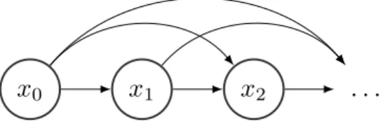
4.2 A probabilistic graphical model corresponding to autoregressive model. This graph represent a trivial connectivity, it is fully connected. . . 55

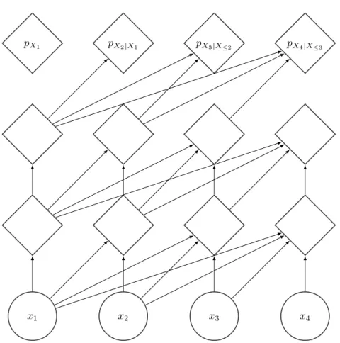
4.3 An example of autoregressive masking pattern, the computational graph represented going bottom up. We see that there is no path connecting xk to p(xk | x<k). . . 56

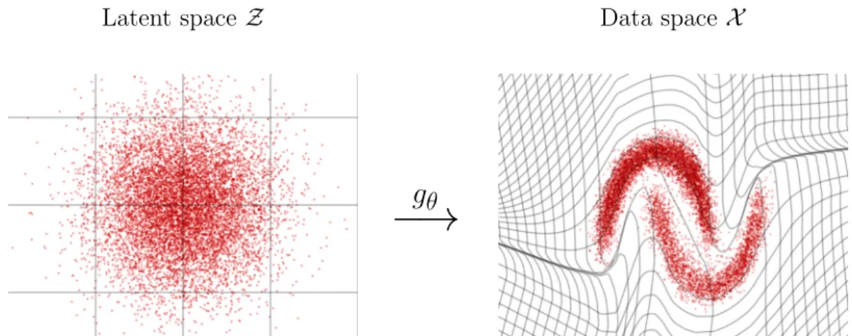
4.4 A generator network approach follows the spirit of inverse transform sampling: sample from a simple distribution a noise variable z, and pass it through the generator network gθ to obtain a sample x =

gθ(z) with the desired distribution. In this example, the desired

distribution is the two moons dataset, which exhibit two interesting properties in its structure: the separation into two clusters, and the nonlinear correlation structure among each cluster. . . 57

4.5 Graphical model corresponding to the emission model: a latent noise variable z is generated from a standard distribution, this variable is then used to build the parameters of the conditional distribution pθ,X|Z. . . 58

4.6 The Helmoltz machine uses an inference network to output an ap-proximate posterior for variational inference qλ(· | x). . . 60

(9)

4.7 An illustration of the reparametrization trick. Considering z as a random variable sampled from a conditional distribution qλ(z | x)

(e.g. N (· | µλ(x), σλ(x))) results in using the Reinforce estimator.

However, by rewriting z as deterministic function of x and a stochas-tic standard variable ϵ (e.g. µλ(x) + σλ(x) with z ∼ N (· | 0, IdZ)),

we can estimate a potentially lower variance gradient estimate by backpropagation. . . 63

5.1 Real NVP _{follows the generator network paradigm (first line with} red figures): gθ transforms a prior distribution (here standard

Gaus-sian) into an approximation of the data distribution. The training of the model is very similar to expectation maximization as the func-tion fθ provides the inference for z given a data point x (second line

with blue figures). However, the generator function here is not only deterministic but also invertible (bijective to be more precise): there is only one latent vector z corresponding to x. The transformations are demonstrated on a model trained on the two moons dataset. Best seen with colors. . . 66

5.2 Computational graphs (from bottom up) corresponding to the for-ward pass of an aﬃne coupling layer and its inverse. . . 69

5.3 Computational graph of a composition of three coupling layers (each represented by a dashed blue box), from left to right. In this alter-nating pattern, units which remained identical in one transformation are modified in the next. . . 71

5.4 The computational graph of a variational autoencoder is very similar to the composition of two coupling layers, with the encoder in red and the decoder in blue. From that observation, on can conclude that not only variational autoencoders maximize a lower bound on the marginal distribution log!pθ(x)", they maximize directly a joint

distribution log!pθ,λ(x, ϵ)". . . 72

5.5 Unbiased samples from a trained model from section 5.2. We sample z _{∼ p}Z and we output x = gθ(z). Although the model is able to

model reasonably the MNIST and TFD datasets, the architecture fails to capture the complexity of the SVHN and CIFAR-10 datasets. 76

5.6 Sphere in the latent space. This figure shows part of the manifold structure learned by the model. . . 77

(10)

5.7 Inpainting experiments. We list below the type of the part of the image masked per line of the above middle figure, from top to bot-tom: top rows, bottom rows, odd pixels, even pixels, left side, right side, middle vertically, middle horizontally, 75% random, 90% ran-dom. We clamp the pixels that are not masked to their ground truth value and infer the state of the masked pixels by Langevin sampling. Note that random and odd/even pixels masking are the easiest to solve as neighboring pixels are highly correlated and clamped pixels gives therefore useful information on global structure, whereas more block structured masking results in more diﬃcult inpainting problems. 78

5.8 Examples of convolution compatible masking for coupling layers. Black dots would correspond to the partition I1 whereas the white

ones would correspond to _I2. . . 79

5.9 Invertible downsampling operation. We break down the images into 2× 2 non-overlapping patches of c channels and convert them into 1_{× 1 patches of 4c channels through reshaping. In this figure, c = 1.} 80

5.10 Shortcut connections for factored out components. We can discard components while conserving the the bijectivity of the function if we add shortcut connections from those discarded components to the final output through concatenation. . . 82

5.11 Multi-scale architecture. We recursively build this architecture by applying three aﬃne coupling layers with checkerboard masking be-fore performing invertible downsampling and applying three aﬃne coupling layers with channel-wise masking. We discard half of the channels of the output (as in figure 5.10). We then repeat this op-eration until the result is 4_{× 4.} . . . 84

5.12 On the left column, examples from the dataset. On the right column, samples from the model trained on the dataset. The datasets shown in this figure are in order: CIFAR-10, Imagenet (32_{× 32), Imagenet} (64× 64), CelebA, LSUN (bedroom). . . 86

5.13 We exploit the convolutional structure of our generative model to generate samples _{×10 bigger than the training set image size. The} model perform best on random crops generated datasets like LSUN categories. . . 87

5.14 Manifold generated from four examples in the dataset. Clockwise from top left: CelebA, Imagenet (64× 64), LSUN (tower), LSUN (bedroom). . . 88

5.15 Ablation of the latent variable by resampling components. Here we

represent the computational graph for generating gθ!(ϵ(1)_I₂, ϵ(2)_I₂, z(3)_I₂, z_I(4)₂ , z(5))". 90

(11)

5.16 Conceptual compression from a model trained on CelebA (top left), Imagenet (64_{× 64) (top right), LSUN (bedroom) (bottom left), and} LSUN (church outdoor) (bottom right). The leftmost column rep-resent the original image, the subsequent columns were obtained by storing higher level latent variables and resampling the others, stor-ing less and less as we go right. From left to right: 100%, 50%, 25%, 12.5%, and 6.25% of the latent variables are kept. . . 91

(12)

List of Tables

5.1 Architecture and results for each dataset. # hidden units refer to the number of units per hidden layer. . . 74

5.2 Bits/dim results for CIFAR-10, Imagenet, LSUN datasets and CelebA. Test results for CIFAR-10 and validation results for Imagenet, LSUN and CelebA (with training results in parenthesis for reference). . . 85

(13)

List of Abbreviations

AdaM _{Adaptative Moment estimation}

AE Auto-Encoder

CDF Cumulative Distribution Function

DNN Deep Neural Network

CNN Convolutional Neural Network

ELBO Evidence Lower BOund

GD Gradient Descent

GMM Gaussian Mixture Model

HMM Hidden Markov Model

KL Divergence Kullback-Liebler Divergence KLD Kullback-Liebler Divergence

LISA Laboratoire d’Informatique des Syst`emes Adaptifs

LSTM Long-Short Term Memory

MoG Mixture of Gaussians

MADE Masked Autoencoder for Density Estimation MCMC Markov Chain Monte Carlo

MDL Minimum Description Length

MILA Montr´eal Institute of Learning Algorithms MLE Maximum Likelihood Estimation

MLP Multi-Layer Perceptron

MSE Mean Squared Error

NADE Neural Autoregressive Density Estimator

NICE Nonlinear Independent Components Estimation NLL Negative Log-Likelihood

PAC Probably Approximately Correct PMF Probability Mass Function PDF Probability Density Function

Real NVP _{Real-valued Non-Volume Preserving} RNN Recurrent Neural Network

SGD Stochastic Gradient Descent VAE Variational Auto-Encoder

(14)

Acknowledgments

you will take the long way to get to these Orions. the long way will become a theme in your life, but a journey you learn to love.

SolangeKnowles(2017) This doctoral program has been a tremendous opportunity to work on a research topic I was passioned about in the blooming field of deep learning. Pursuing this en-deavor would not have been possible without the consistent support of my family, friends, colleagues, and advisors.

I want to thank Professor and CIFAR Senior Fellow Yoshua Bengio for communicating his passion for artificial intelligence, welcoming in and guiding me through an internship and a doctoral program, and for his patience and support, which allowed me to set up my own research agenda and style, and learn to manage community expectation and my own.

Following the impressive growth of deep learning, the lab I was navigating in under-went a radical structural transformation. I want to thank organizers of this lab, Céline Bégin, Linda Penthière, Angela Fahdi, Jocelyne Étienne, and Myriam Côté, for mak-ing this growth possible. I also want to thank friends, collaborators, co-workers, and colleagues who contributed to the different phases MILA (formerly known as LISA) un-derwent, with whom I had the pleasure to have fruitful interactions, in terms of work or learning experience, who provided moral support, and who shared their enthusiasm for their craft, including: Aaron Courville, Adriana Romero, Adrien Ali Ta¨ıga, Ahmed Touati, Alexandre De Brébisson, Amar Shah, Amjad Almahairi, Amy Zhang, Anna Huang, Antti Rasmus, Arnaud Bergeron, Asja Fisher, Atousa Torabi, Bart van Merriën-boer, ¸Ca˘glar Gül¸cehre, César Laurent, Chiheb Trabelsi, Chin-Wei Huang, Daniel Jiwoong Im, David Krueger, David Warde-Farley, Devon Hjelm, Dmitriy Serdyuk, Dustin Webb,

(15)

Dzmitry Bahdanau, Eric Laufer, Faruk Ahmed, Felix Hill, Francesco Visin, Frédéric Bastien, Gabriel Huang, Grégoire Mesnil, Guillaume Alain, Guillaume Desjardins, Harm De Vries, Harri Valpola, Ian Goodfellow, Ioannis Mitliagkas, Ishaan Gulrajani, Jacob Athul Paul, Jessica Thompson, João Felipe Santos, Jörg Bornschein, José Sotelo, Juny-oung Chung, Kelvin Xu, Kratarth Goel, Kyunghyun Cho, Kyle Kastner, Li Yao, Marcin Moczulski, Mathias Berglund, Mathieu Germain, Mehdi Mirza, Mélanie Ducoffe, Mo-hammad Pezeshski, Negar Rostamzadeh, Nicolas Ballas, Orhan Firat, Pascal Lamblin, Pascal Vincent, Razvan Pascanu, Saizheng Zhang, Samira Shabanian, Simon Jégou, Si-mon Lefran¸cois, SiSi-mon Lacoste-Julien, Sungjin Ahn, Tapani Raiko, Tegan Maharaj, Tim Cooijmans, Thomas Le Paine, Valentin Bisson, Vincent Dumoulin, Xavier Glorot, Yann Dauphin, Yaroslav Ganin, and Ying Zhang.

My visits in different research groups (machine learning group in University of British Columbia, Google Brain, and DeepMind) also provided me with valuable opportunities to learn and build a more unique research agenda. Thanks to Samy Bengio, Nando de Freitas, and Helen King for inviting me in their research groups and providing su-pervision. I am also grateful to the friends, collaborators, co-workers, and colleagues I met during these visits or in conferences. They provided productive collaborations, welcomed me in their group, shared valuable insights and experiences, or inspired by their contribution, among them: Aäron van den Oord, Andrew Dai, Anelia Angelova, Angeliki Lazaridou, Ariel Herbert-Voss, Arvind Neelakantan, Aurko Roy, Babak Shak-ibi, Ben Poole, Bobak Shahriari, Brandon Amos, Brendan Shillingford, Brian Cheung, Charles Frye, Chelsea Finn, Danielle Belgrave, Danilo Jimenez Rezende, David Ander-sen, David Grangier, David Ha, David Matheson, Deirdre Quillen, Diane Bouchacourt, Durk Kingma, Édouard Oyallon, Edward Grefenstette, Emmy Qin, Eric Jang, Eugene Belilovsky, Gabriel Synnaeve, Gabriella Contardo, Georgia Gkioxari, George Edward Dahl, Grzegorz Swirszcz, Hugo Larochelle, Ilya Sutskever, Irwan Bello, Jackie Kay, Jamie Kiros, Jascha Sohl-Dickstein, Jean Pouget-Abadie, Johanna Hansen, Jon Gauthier, Jon Shlens, Joost Van Amersfoort, Junhyuk Oh, Justin Bayer, Karol Hausman, Konstanti-nos Bousmalis, Luke Vilnis, Maithra Raghu, Marc Gendron Bellemare, Mareija Baya, Matthew Hoffman, Matthew W. Hoffman, Max Welling, Mengye Ren, Mike Schuster,

(16)

Misha Denil, Mohammad Norouzi, Moustapha Cissé, Naomi Saphra, Nal Kalchbrenner, Natasha Jaques, Navdeep Jaitly, Neha Wadia, Nicolas Le Roux, Nicolas Usunier, Nicole Rafidi, Olivier Pietquin, Oriol Vynials, Peter Xi Chen, Pierre Sermanet, Pierre-Antoine Manzagol, Prajit Ramachandran, Quoc Viet Le, Rafal Jozefowicz, Rahul Krishnan, Raia Hadsell, Rémi Munos, Richard Socher, Rupesh Srivastava, Sam Bowman, Sander Diele-man, Scott Reed, Sergio Gómez Colmenarejo, Shakir Mohamed, Sherry Moore, Simon Osindero, Soham De, Stephan Gouws, Stephan Zheng, Shixiang Shane Gu, Taesung Park, Takeru Miyato, Tejas Kulkarni, Théophane Weber, Tim Salimans, Timnit Gebru, Tina Zhu, William Chan, Wojciech Zaremba, Yannis Assael, Yutian Chen, Yuke Zhu, Zhongwen Xu, and Ziyu Wang.

I thank as well my teachers who prepared me for this program: Arnak Dalalyan, Erick Herbin, Gábor Lugosi, Gilles Faÿ, Guillaume Obozinski, Iasonas Kokkinos, Igor Kornev, Jean-Philippe Vert, Laurent Cabaret, Laurent Dumas, Lionel Gabet, Matthew Blaschko, Michael I. Jordan, Nicolas Vayatis, Nikos Paragios, Patrick Teller, Pauline Lafitte, Pawan Kumar, and Rémi Munos.

I am also grateful for the suport of my family, not only my parents I am in debt to but also my siblings Huy, Ho`a, and Laura, and my cousins, including Isabelle, Lucie, Laura, and Arthur.

Thanks to my friends who kept me grounded and without whom I wouldn’t be here, particularly: Alexandre, Ansona, Antoine, Amanda, Amin, Audrey, Baptiste, Charlotte, Claire, Diane, Fabien, Florence, Guillaume, Hadrien, Ibrahima, Jean-Charles, Jessica, Johanna, Loic, Marguerite, Martin, Mathilde, Nicolas, Nicole, Rebecca, S´evan, Tarik, Thomas, and Vincent.

Thank you Nicolas Chapados for providing the thesis template, and Kyle Kastner and Junyoung Chung for showing me how to use it. Additionally, I’m grateful to Juny-oung Chung, Adriana Romero, Harm De Vries, Kyle Kastner and ´Edouard Oyallon for providing feedback to this dissertation.

Finally, the work reported in this thesis would not have been possible without the financial support from: Ubisoft, NSERC, Calcul Quebec, Compute Canada, the Canada Research Chairs and CIFAR.

(17)

1

_{Machine learning}

Computer science can be defined as the study and application of eﬃcient auto-matic algorithmic processes. This field has known unreasonable eﬀectiveness in its application to domains like commerce, finance, entertainment, logistics, and educa-tion through by enabling the automaeduca-tion of simple tasks such as querying, storing, and processing data at impressive scale.

However, most of these algorithmic processes were traditionally implemented through direct programming. As direct programming involved careful writing of explicit handcrafted rules, logics, and heuristics, researchers soon realized that such traditional approach proved to be too cumbersome for tasks like computer vision and natural language processing to be eﬃcient. Indeed, although these problems were mostly trivial for the average neurotypical, able-bodied person, manually de-signing good solutions was near impossible.

The work presented in this thesis has been done in the framework of machine learning. Machine learning is a subfield of computer science that aimed to address this shortcoming in direct programming. Instead, it would enable to specify non-constructively a solution to these problems through examples of correct behaviors. The model would then learn on that data to obtain the desired behavior.

The recent increase in data production and computational power that happened in the last few decades was a key component in the success of this approach and appropriately addressed new challenges in information processing and automation brought by this surge, now making machine learning an important, if not essential, part of computer science.

I will introduce machine learning briefly in this chapter but further details on the concept can be found in Bishop (2006); Murphy(2012); Goodfellow et al.(2016).

(18)

1.1 Definition

Machine learning is the study of systems that can adapt and learn from data. This paradigm becomes particularly useful when collecting a large amount of data on these complex tasks can prove to be more productive and less human labor intensive than hand-crafting programmed behaviors. Relying instead on increasing computing power, machine learning would, in this situation, harness this large amount of data to induce a set of behaviors to solve these problems.

More formally, machine learning is characterized by the ability to “learn from experience E with respect to some class of tasks T and performance measure P“, i.e. “its performance at tasks in T , as measured by P , improves with experience E“ (Mitchell, 1997). Since the said experience, tasks, and performance measure largely vary depending on the problem at hand, I will specify and detail the domains we are interested in.

Experience The nature of the experience of a machine learning algorithm will be numerical. Often the numbers presented to this algorithm will take the form of a set of elements in an input domain X , which is usually finite sequences of scalars or vectors. The domain can be a finite set of elements, scalar R, vector space RdX _{(with dX} _{the data dimensionality), finite sequences of these domains} #

m∈N+(Xsub)m, or any combination of these domains. Most commonly, the base domain will be a vector space Rd_Xsub_{, each element of a vector of that domain are} called a feature. In supervised learning, this domain is supplemented with an output domain _Y.

A common assumption on these series is that they are independently and iden-tically distributed, meaning each example is drawn independently from the same data distribution p∗

X. This assumption is often essential in establishing the gener-alization capability of most machine learning algorithms.

Task Machine learning algorithms can be used on a large array of problems. These problems are often reframed in a more abstract task including supervised learning and unsupervised learning tasks. Supervised learning tasks are charac-terized by its goals of finding a mapping f from input space _{X to output space} Y. The output space for classification, regression, and structured prediction are

(19)

respectively a finite set, scalar, or a subset of finite sequences of these domains. Unsupervised learning aims at characterizing the input space distribution itself in some meaningful way, including density estimation, clustering, or imputation of missing values.

Performance measure One key component in describing a problem in machine learning is the performance measure we aim to optimize. More often, we minize instead its opposite, the loss function L(f). In our case, the loss function can be decomposed into a corresponding value ℓ(f, x) for each element x∈ X (or ℓ(f, x, y) for each pair (x, y)_{∈ X ×Y), resulting in an expression of the loss as the expectation}

L(f, p∗X) = Ex∼p∗X[ℓ(f, x)] = $ x∈X ℓ(f, x) dp∗X(x) or _{L(f, p}∗_X,Y) = Ex,y∼p∗ X,Y[ℓ(f, x, y)] = $ (x,y)∈X ×Y ℓ(f, x, y) dp∗_X,Y(x, y).

A common loss function in classification is for example the 0-1 loss: ℓ01(f, x, y) = 1 (f (x) = y).

Given these definitions, the task of learning consists in finding a good, if not optimal, behavior among a set_{F of possible functions, called the hypothesis space,} in order to minimize this expected loss _{L(f, p}∗

X) = Ex∼p∗X[ℓ(f, x)], also called the expected risk.

However, this data distribution over which the expectation would be computed is not directly provided to the system. Instead, the system is only provided with a finite amount of data D = (x(n)_)n≤N _{∈ X}N _{that will allow the model to properly} infer a correct behavior. One way to find an approximate solution is empirical risk minimization (Vapnik,1992), where we minimize a Monte Carlo approximation of the expected loss called the empirical loss (also known as empirical risk, Vapnik,

2013), ˆ L(f, D) = _N1 N % n=1 ℓ(f, x(n)).

(20)

optimiza-tion in the hope that this minimizaoptimiza-tion will result in a reasonable soluoptimiza-tion with respect to the expected loss, which we also call the generalization error. This gen-eralization loss is also estimated by Monte Carlo using separate data from the same distribution1_{. To this eﬀect, the data is often separated in at least two subsets, the}

training subset Dtrain, on which the algorithm is trained, and the test subset Dtest, on which the expected loss is estimated.

1.2 Examples

1.2.1 Linear regression

One of the simplest examples of machine learning problem is the scalar linear regression problem. As the name indicates, the class of functions used will be the set of linear functions from RdX _{'→ R (see figure} _1.1b_),

Flinear = & f : x = (xi)i≤d_X _'→ dX % i=1 wi_{· x}i,_{∀w = (w}i)i≤d_X _{∈ R}dX ' .

In reality, we are considering the set of aﬃne functions in RdX '→ R, which would be equivalent to linear functions on the augmented vectors ˜x = (1, x0, . . . , xd_X).

Let_{D = (x}(n)_{, y}(n)_)n≤N _{∈ (R}dX_{, R)}N_{, the loss we aim to minimize in this} regres-sion problem is the mean squared loss (see figure 1.1a)

ˆ LM SE(f,D) = 1 N N % n=1 !f(x(n)₎_{− y}(n)"2 ˆ LM SE(w,D) = 1 N N % n=1 (< x(n)_{, w >}_−y(n)₎2_.

Although the linear function hypothesis space is so limited that it would rarely contain the data generating behavior in most realisitic cases, it allows for closed form solution inference. Let X be the design matrix, a matrix of size n× d whose

1

We don’t consider in this dissertation the important case of transfer learning when the ob-jective is loss minimization on another distribution.

(21)

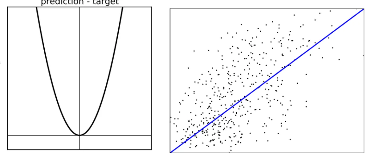
(a) Plot of the quadratic loss with re-spect to the diﬀerence between the pre-diction and the target.

(b) A 2-D visualization of a trained linear re-gression model with the associated data points. The learned relationship between input and output is constrained to be aﬃne. In some cases (including this one), that it enough.

Figure 1.1 – Visualization of a trained linear regression model with the associated loss function.

rows are corresponding to the vectors (x(n)_)n≤N_{, and y}_{∈ R}N _{the vector containing} each corresponding value (y(n)_)n≤N_{. The loss function can be rewritten}

ˆ LM SE(w,D) = 1 N(Xw T − yT )T(XwT − yT ) which is minimized when its derivative with respect to w is zero

∂ ˆLM SE(w,D) ∂wT = 1 N(Xw T − yT_{) = 0} ⇒ XT_XwT _{= X}T_yT ⇒ wT _{= (X}T_X)−1_XT_yT_.

1.2.2 Logistic regression

Despite its name, logistic regression is a classification problem, meaning that the data of interest D = (x(n)_{, y}(n)_)n≤N _{is in (R}dX_,{0, 1})N _{for the binary case.} The class of function is still Flinear but instead of predicting values directly the predictor will output a score for ”positive” label 1, we then follow the plug-in rule: if the score is positive then the prediction will be 1, otherwise it will be 0.

(22)

(23)

mization techniques. Unfortunately, both assume some degree of linearity in the problem, which is a very limited case. These algorithms are lacking expressive power.

A decomposition of the generalization error in Bottou and Bousquet (2008) provides insight on the desiderata of machine learning approaches. Let’s consider an hypothesis space F, A a stochastic algorithm which take a dataset D as in-put to return a predictor ¯f ∈ F by approximate empirical risk minimization,

ˆ

f = arg minf∈F !ˆ

L(f, D)"

∈ F a solution to empirical risk minimization in the family _{F, f}∗

F = arg minf∈F!L(f)" an optimal predictor with respect to the gener-alization error in the family_{F, and f}∗ _{= arg min}

f !L(f)" the optimal predictor for generalization (not necessarily in _{F), then} Bottou and Bousquet (2008) proposes the following decomposition:

E(L( ¯f )) =E*_{L( ¯}_{f )}_{− L( ˆ}_{f )}+ +E * L( ˆf )_{− L(f}_F∗)+ +E_[_L(f∗ F)− L(f∗)] + E [_L(f∗)] .

E_[_L(f∗_{)] is the irreducible error you can have in a problem and computing this} quantity requires generally to find the solution f∗_{. In that decomposition, the other} terms are: E [_L(f∗

F)− L(f∗)] is called the approximation error, E *

L( ¯f )_{− L( ˆ}f )+ is theoptimization error, and E*_{L( ˆ}f )_{− L(f}∗

F) +

is theestimation error. To follow the nomenclature ofRaghu et al.(2017), these terms correspond to theexpressivity,

trainability, and generalizability of a model.

1.3.1 Expressivity

One necessary condition for meaningful learning is to be flexible enough to adapt to training data. As mentioned earlier, the previous linear models (logistic regression and linear regression, see figure 1.1b and 1.2b) are however unlikely to include the optimal predictor f∗ _{for most interesting problems. If the problem is on} the contrary very nonlinear, such model are likely to underfit, i.e. not being able to approximate well the solution regardless of the quantity of data and computation. It is in general the case that the hypothesis space picked in our machine learning

(24)

algorithm does not include f∗_{and therefore introduces a bias in the solutions found.} Given that observation, we woud like to adopt a family of predictors that would include a good enough approximation of f∗_.

This is often done by increasing the model capacity to approximate diﬀerent functions. To that eﬀect, one could increase the number of features when specifying the model, increase the expressivity of a kernel function in shallow learning, or increase the size of a neural network in deep learning. The more functions a model can approximate the more powerful we consider it.

1.3.2 Trainability

If the eﬀectiveness of a machine learning model was solely defined by its expres-sivity, a simple solution would be to arbitrarily increase model capacity to minimize the approximation error. However, one of the hurdles practioners would face with that approach is the finite computational resources at hand.

Machine learning methods related to empirical risk minimization are generally doing a search of the hypothesis space in order to approximately minimize a loss function. The larger and complex this hypothesis space, the less eﬀective that search will be. For example, loss functions involving neural networks are notoriously non-convex in general, making the use of a convex optimization algorithm less reliable. Practical restriction in the ability to fully explore the hypothesis space results in a decrease in the eﬀective capacity of a model.

Inference in the chosen model has to be at least tractable, i.e. computable in reasonable time, making a naive approach to memory-based learning (or instance-based learning) hardly scalable with the size of the dataset. Therefore it is here essential for machine learning models to discover reliable patterns and redundancy in the data to reduce in order to decrease unnecessary computation or memory usage.

1.3.3 Generalizability

Another reason to discover these patterns and redundancy is that they also en-able meaningful learning. Generalization is a central question in machine learning: if the model was only able to extract information about the training data but could not extrapolate to new examples, the predictor would be hardly useful. Aimlessly

(25)

increasing a model’s effective capacity often results in discovering and focusing on coincidental spurious patterns, i.e. noise, from the training set on which we do em-pirical risk minimization. As a result, the estimation error increases. We call this effect overfitting. The solution obtained from training on the Monte Carlo estimate of the expected loss is said to have high variance: the predictor is more a function of the particular instantiation of the dataset than of the task itself. A more com-mon quantity to measure overfitting is the difference between generalization loss and training loss, called the generalization gap,

L(f) − ˆL(f, Dtrain).

Under scalability constraints, increasing the amount of data used, artificially augmenting the data if necessary, reduces that variance reliably. If our model is consistent, it will converge to the true model f∗ by definition. But collecting more data by an order of magnitude can be very expensive and time-consuming.

A way to overcome the variance of the resulting predictor is to average an ensemble of several valid hypotheses. One could, for example, implement boostrap aggregation (Breiman,1996) (also known as bagging) and train on a few instances of the same model on diﬀerent subsets of the training set. Bayesian inference (Neal,

2012; Andrieu et al., 2003; Solomonoﬀ, 1978) averages on every valid hypotheses reweighted by their relevance according to an a priori knowledge and the training set.

Under that same computation budget, limiting the computation can also prove to be eﬀective in reducing overfitting, but possibly at the cost of increased bias. Reducing model capacity is an example of such approach. One could also reduce the eﬀective capacity by adding stochasticity in model search or model inference.

The model search can also be guided towards simpler hypotheses. For example, one can augment empirical risk minimization with a regularization term or penalty term, i.e. a term that aims at eﬀectively bridging the diﬀerence between the em-pirical risk and the expected risk, in a similar fashion as the classic generalization bounds from statistical learning theory, resulting in the regularized empirical risk minimization problem

ˆ

(26)

We call regularization the process of reducing (eﬀective) model capacity in order to increase generalizability.

Since using such regularization would hinder performance on the training set, the regularization needs either to be decided prior to any training or tuned using a held-out subset of the dataset. Since the test setDtest must remain unused until final evaluation (e.g. Dwork et al., 2015), one should use instead a third separate subset, which is traditionally called the validation set Dvalid.

1.3.4 Tradeoﬀ

Although bias, computation, and variance can be arbitrarily separated to un-derstand phenomena in machine learning, they remain ultimately entangled in a bias-variance-computation tradeoff. The figure1.3shows the bias-variance tradeoff, a subset of this bias-variance-computation tradeoff.

Ideally, we wish to have an algorithm which will perform well on all counts: the model must be expressive, tractable, and generalize well. Now the infamous no free lunch theorem (Wolpert, 1996) states that no general purpose algorithm can fulfill those desiderata. Therefore, to enable the design of eﬃcient learning algorithms, one must aim at restricting the set of tasks they want to solve. The less exhaustive is this set, the more opportunities we would have to provide a model with the appropriate inductive bias.

Figure 1.3 – A cartoon plot of the generalization loss with respect to the effective capacity. The blue line is the training loss, the red one is the generalization gap, and their sum, thegeneralization loss is in purple. This plot illustrate the bias-variance tradeoff: although increasing effective capacity decreases the training error, it increases the generalization gap. Although increasing effective capacity reduces training error, the return is decreasing exponentially. On the other hand, the incurred varianceof the estimated solution ˆf can increase with capacity to the point where the model is effectively useless. As a result, thegeneralization loss(in purple) is minimized in the middle. Best seen with colors.

(27)

(28)

2

_{Deep learning}

2.1 The hypothesis space

Bengio et al. (2007) define an AI-set of tasks of interest. These tasks includes perception, control, and planning. The raw sensory input involved in those tasks are typically high dimensional, e.g. a mere color image of size 64_{× 64 already results} in vectors of more than 10, 000 dimensions. As a a result, we are encountering a curse of dimensionality in these problems, when expressivity, trainability, and generalizability degrade exponentially with the number of dimensions.

A key ingredient in enabling learning on these problems is to exploit their reg-ularities. A starting point for local generalization (i.e. around data points) is to embed the system with a smoothness prior : nearby points should have similar prop-erties in terms of labeling and density1_{. This prior can be strengthened by taking}

advantage of the dominant structure of the data. In particular, one characteristic we hope to exploit in these tasks is the relatively low intrinsic dimensionality of the data. For instance, natural images remain around a data point predominantly along specific directions. This assumption is called the manifold hypothesis.

An eﬃcient learning algorithm would hopefully be able to obtain global gen-eralization (i.e. outside the immediate vicinity of data points). Whereas purely local template matching algorithms would resort to one-hot representations (an extremely sparse vector with only one non-zero component) deep learning (Bengio,

2009;Goodfellow et al.,2016) exploits the notion of distributed representation ( Hin-ton,1984), where information is instead distributed across multiple dimensions. An example of such distributed distribution would be a binary representation for a set of N integers, which takes less space than a one-hot binary representation (log₂(N ) instead of N ).

An ideal outcome would be to successfully disentangle factors of variation into 1

In hindsight, the existence of adversarial examples (Szegedy et al., 2014; Goodfellow et al.,

2015) in recent deep learning systems shows how weak such inductive bias is in those systems.

(29)

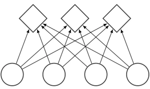
Figure 2.1 – Computational graph of a feedforward neural network layer. The computation goes upward, the botton nodes are the inputs and the top nodes are the outputs. Each output node take all the input with diﬀerent strength (defined by the weight matrix), before applying a nonlinearity if necessary.

diﬀerent features, which would allow an eﬃcient reusability of these disentan-gled features. Such features facilitate global generalization by sharing statistical strength, by exploiting recombinations of the properties of training examples, one can extrapolate outside their vicinity.

2.1.1 Artificial neural networks

A key component in learning those distributed representations are artificial neu-ral networks, composed typically from feedforward layers with functional equation

h = φact(xW + b)

where h is a vector output, the result of an aﬃne operation, represented by the matrix W , called the weights, and a vector b called the oﬀset, composed with an element-wise activation function φact, which can be

• the identity function, the layer is then called linear 2_;

• the logistic sigmoid function (figure 2.2a)

φsigmoid(x) = !1 + exp(−x)"−1;

• the hyperbolic tangent function (figure 2.2b)

φtanh(x) = 2 φsigmoid(2x)− 1; 2

If the neural network is solely a composition of linear layers, then it can only express linear functions.

(30)

(a) Logistic sigmoid (b) Tangent hyperbolic (c) Rectified linear

Figure 2.2 – Examples of activation functions.

• the rectified linear function (Jarrett et al.,2009;Nair and Hinton,2010;Glorot et al., 2011) (figure 2.2c)

φrect(x) = max(0, x).

These feedforward layers can typically be composed obtain the desired predic-tion following the recurrence

h(k+1)= φact,(k)(h(k)W(k)+ b(k))

where h(0) _{would be the input x of the artificial neural network and for k > 0, h}(k) would be called a hidden layer, with the exception of the last, which would be the output layer. Each dimension of these hidden vectors are typically called neurons, to follow the neural network analogy, which are connected by these weights W(k) (see Figure2.1). When none of the element of the weight matrix is constrained to be 0, then we call the corresponding layer fully-connected.

Although the default parametrization of such layer is to make the affine oper-ation arbitrary, there is value in exploiting the particular structure in signals of interest. For instance, the local structure and limited translation equivariance of natural images and sound signals enables us to restrict this affine transformation to be a discrete convolution (LeCun and Bengio,1994;Kavukcuoglu et al.,2010) (see also Dumoulin and Visin, 2016), resulting in improving generalization by limiting the hypothesis space, and computational efficiency, both memory-wise parameter sharing across the signal and computation time as convolution involves less

(31)

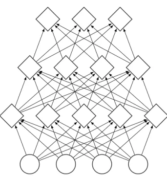
Figure 2.3 – Computational graph of a deeper feedforward neural network. The computation goes upward, the botton nodes are the inputs and the nodes above are the hidden and output units. Each hidden and output node take all the input from previous layer with diﬀerent strength (defined by the weight matrix), before applying a nonlinearity if necessary.

putation (because of the underlying sparse connectivity) that can be more easily parallelized.

2.1.2 Powerful architecture

For some non-linear activation functions, even a one hidden layer neural network can approximate any continuous function with arbitrary precision on a bounded set given that this hidden layer is suﬃciently large, this result is known as the universal approximation theorem (e.g.Cybenko,1989;Hornik,1991;Barron,1993), grounding further the intuition in subsection 1.3.1 that increasing the size of the model by adding hidden units does indeed improve its capacity.

However, this capacity might come at an unbearable cost in terms of computa-tion and generalizacomputa-tion for shallow models, even when exploiting parallel compu-tations. Several arguments have been made (e.g. Bengio et al., 2006; Bengio and Delalleau, 2011;Martens and Medabalimi,2014; Montufar et al.,2014; Eldan and Shamir,2016;Poole et al.,2016;Raghu et al.,2017;Telgarsky,2016) demonstrating the eﬀectiveness of favoring deep architectures, i.e. models with many layered com-putations, over shallow ones, i.e. models with fewer of these layers. The argument

(32)

(33)

algorithm (Rumelhart et al., 1988), which combines the chain rule for derivatives with dynamic programming. If we consider the layer

h(k+1)= φact,(k)(h(k)W(k)+ b(k)) then the gradients follow the recursive equation

∂L ∂(W(k)₎T = φ ′ act,(k)(h(k)W(k)+ b(k))⊙ (h(k))T · ∂L ∂(h(k+1)₎T ∂L ∂(b(k)₎T = φ ′ act,(k)(h(k)W(k)+ b(k))⊙ ∂L ∂(h(k+1)₎T ∂L ∂(h(k)₎T = φ ′ act,(k)(h(k)W(k)+ b(k))⊙ ∂L ∂(h(k+1)₎T ·!W (k)"T

where ⊙ is the element-wise multiplication.

While the h(k) _{quantities are computed through the forward computation, the} ∂L

∂(h(k)₎T are computed during the backward computation of the derivative. As the forward computations are stored in memories, the computation of these derivatives are as eﬃcient as the forward computation. These functionalities are implemented in frameworks including automatic diﬀerentiation toolkits like Theano (Bergstra et al., 2010;Bastien et al.,2012) and Tensorflow (Abadi et al., 2016).

2.2.2 Stochastic gradient descent

The iterative (batch) gradient descent algorithm (illustrated in figure 2.5) lays the foundation of most gradient-based algorithms used in deep learning. The al-gorithm proceeds as follow to follow a loss LDtrain = ˆL(·, Dtrain): we start from a given initialization (possibly random) of the parameter θ0 ∈ Θ and at each step t we update the parameter by substracting a vector proportional to the gradient

∂L_Dtrain

∂θt (θt), scaled by a positive factor αt called the learning rate. An advantage with iterative algorithms is their ability to be interrupted at any step on their way to a local minimum and still provide in theory a decent approximate solution given the computational budget. Moreover, in several successful deep learning models, even a local minimum can often reach very good performance.

(34)

(35)

A computational hurdle with batch gradient descent however is that computing the gradient requires computing

LDtrain(θt) = 1 |Dtrain| % x∈Dtrain ℓ(θ, x),

which remains ultimately linear with the size of the training set, which can still be too expensive as a significant number of steps need to be taken in order to reasonably approximate a minimum. Fortunately, for a uniformly and randomly selected subset ˆMtrain of Dtrain, if we note

L_Mtrainˆ (θt) = 1 | ˆMtrain| % x∈ ˆMtrain ℓ(θ, x), then ∂LMtrainˆ

∂θt (θt) is an unbiased stochastic approximation of

∂L_Dtrain ∂θt (θt) E _ˆ Mtrain ,_∂ LMtrainˆ ∂θt (θt) -= ∂LDtrain ∂θt (θt)

whose computational cost becomes linear with the size of the subset ˆMtrain, which we call mini-batch. Because it uses a stochastic approximation of the gradient instead of the exact estimate, this variant is called stochastic gradient descent ( Er-moliev, 1983) (described in Algorithm 2). Under mild assumption, this algorithm converges to a local minimum, even for a mini-batch of size 1 (Robbins and Monro,

1951; Bottou, 1998). There are of course tradeoﬀs to consider when picking the (mini)batch size, a smaller mini-batch will use less computation and memory, and the noise incurred in gradient estimation can result in regularization (Wilson and Martinez, 2003), a larger batch can also help exploit parallelizable computational processes and provide a more accurate estimation of the gradient (Goyal et al.,

(36)

(37)

pure optimization, there are several approaches to tackle this conditioning prob-lem. Momentum (Nesterov et al., 2007; Sutskever et al., 2013) uses a moving average of the stochastic gradient estimate which can counter fluctuation issues for example. One can also precondition the problem, i.e. rearrange its geometry such that the new problem has a more appropriate conditioning, by using second order methods (e.g Amari, 1998; Pascanu and Bengio, 2014; Martens and Grosse,

2015) or adaptative learning rate (e.g Tieleman and Hinton,2012; Dauphin et al.,

2015; Wilson et al., 2017) methods. In particular, we will use Adaptative Moment estimation (AdaM) (Kingma and Ba,2015) (described in Algorithm 3) for train-ing models, despite its issue regardtrain-ing convergence properties (Sashank J. Reddi,

2018).

Algorithm 3 AdaM algorithm

Require: Initialization of θ0 ∈ Θ, learning rate sequence (αt)t≥0 ∈ (R∗ +)

N

, decay coeﬃcients (β1, β2)∈ [0, 1[, damping coeﬃcient ϵ > 0

θ_{← θ}0 µ1 ← 0 µ2 ← 0 t_{← 0}

while not termination(ℓ, θ,Dtrain) do

Sample mini-batch _{M = ˆ}_Mtrain ⊂ Dtrain uniformly µ1 _{← β}1µ1+ (1_{− β}1) (∇θLMˆ) (θ)

µ2 ← β2µ2+ (1−β2) ((∇θL_Mˆ) (θ))⊙2 (gradient estimate squared element-wise) θ ← θ − αt_1−βµ1t+1 1 . 1−β₂t+1 µ2+ϵ t_{← t + 1} end while return θ

2.2.3 Gradient flow

Another view of conditioning in deep learning problem has been the issue of gra-dient flow : as gragra-dient is estimated through backward computation, how much does the signal degrade. In particular, as the gradient is propagated backward, its norm can grow/shrink exponentially, resulting in exploding/vanishing gradients ( Hochre-iter, 1991;Bengio et al.,1994). As this issue becomes more significant with depth, this has been one of the main hurdle in training deep networks.

(38)

Several techniques have helped mitigate this diﬃculty, for instance new ini-tialization techniques (e.g. Glorot et al., 2011; Sutskever et al., 2013; Sussillo and Abbott, 2014). A significant eﬀort has been put into architectural design of deep models in order to improve gradient propagation.

• Glorot et al.(2011) show the advantage of using the rectified linear activation functions in deep neural networks in terms of gradient propagation, whose piecewise linear design enabled better gradient propagation than saturating nonlinearities like logistic sigmoid.

• Batch normalization (Ioﬀe and Szegedy, 2015; Desjardins et al., 2015) inte-grate feature normalization in the forward equation, with moments estimated from the current mini-batch, in order to alleviate gradient propagation issues. • Weight normalization (Badrinarayanan et al., 2015; Salimans and Kingma,

2016; Arpit et al., 2016) reparametrizes the weights as a product of a norm and normalized direction.

• Hochreiter (1991);Bengio et al.(1994) laid the principles to design the long-short term memory (Hochreiter and Schmidhuber, 1997b; Zaremba et al.,

2014) recurrent neural networks (Rumelhart et al., 1988), which in turn was influential in the design of skip connections (Lin et al., 1996), highway net-works (Srivastava et al.,2015), and residual networks(He et al.,2015a,2016). In particular residual networks replace some fully connected feedforward lay-ers with residual blocks with forward equation h(k+1) _{= h}(k) _{+ fres,(k)(h}(k)₎ where fres,(k) is a small and shallow neural network (see figure 2.7). These residual connections possibly solve a shattered gradient (Balduzzi et al.,2017) problem, i.e. when the gradients with respect to the parameters are similar to white noise.

(39)

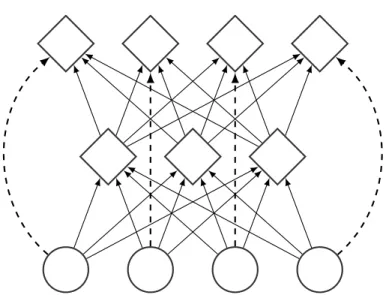
Figure 2.7 – Computational graph of a typical residual block. The output of the small neural network is added to the input. This operation represented by dashed arrows which are called the residual connections.

There is arguably a relationship between architectural design and adaptative gradient methods through reparametrization. If η = Φ−1(θ) a reparametrization of θ (with Φ bijective), then by taking the new loss function L(η)Dtrain =LDtrain ◦ Φ, the gradient in this reparametrized problem has the form

/

∇ηL(η)_Dtrain 0

(η) = (∇θLDtrain) (θ)· (∇ηΦ) (η),

resulting in a diﬀerent gradient descent algorithm (reminiscent of the mirror descent algorithm, Beck and Teboulle, 2003) by manipulation of the problem geometry

θt+1 = Φ(ηt+1) = Φ/ηt− αt / ∇ηL(η)_Dtrain 0 (ηt)0 = Φ!Φ−1_(θt) − αt(∇θLDtrain) (θt)· (∇ηΦ)!Φ−1(θt) "" as shown by Sohl-Dickstein (2012) when Φ is linear.

(40)

2.3 Generalizability of deep learning

Although expressivity and fast computation enabled successful applications of deep learning models to object recognition in images (e.g Krizhevsky et al., 2012;

Goodfellow et al., 2014a; Simonyan and Zisserman, 2015;Szegedy et al.,2015; He et al., 2016, 2017), machine translation (e.g. Cho et al., 2014; Sutskever et al.,

2014; Bahdanau et al., 2015; Wu et al., 2016; Gehring et al., 2016), and speech recognition (e.g. Dahl et al.,2012;Hinton et al.,2012; Graves et al., 2013;Hannun et al.,2014;Chorowski et al.,2015;Chan et al.,2016;Collobert et al.,2016), it does not solely explain their success. In order for learning to succeed, the algorithms need to have some degree of generalizability.

A recent study (Zhang et al., 2017) highlighted the well-known issue that sta-tistical learning theory notions like Vapnik–Chervonenkis dimension (Vapnik and Chervonenkis, 2015) and Rademacher complexity (Bartlett and Mendelson, 2002) used to obtain probably approximately correct (PAC) generalization bounds cannot be applied to deep learning models to obtain useful bounds. Indeed, the only guar-antee they provide is a generalization error lower than 100%, they are therefore called vacuous (Dziugaite and Roy, 2017).

One of the promising approaches to explaining generalization in deep learning is the holistic approach of stochastic approximation (Nesterov and Vial,2008;Bottou et al., 2016), encompassing the joint issues of approximation, computation, and stochasticity. In particular, the notion of uniform stability (Bousquet and Elisseeﬀ,

2002) allowed to explore an interesting path in building generalization bounds in restricted cases (Hardt et al., 2016; Gonen and Shalev-Shwartz, 2017). Unfortu-nately, this approach does not account for the particularity of the problem at hand whereas, as stated earlier, its complexity should modulate the tradeoﬀ between approximation quality, computation, and estimation reliability.

The PAC-Bayes framework (McAllester, 1999; Langford and Caruana, 2001;

Dziugaite and Roy,2017;Neyshabur et al.,2017) provides nonvacuous data-dependent bounds on the generalization gap. It relies on defining an a priori distribution p (i.e. defined before any training) on the parameter θ and a distribution q defined by training, and gives an expression of the generalization gap as function of the

(41)

Kullback-Leibler divergence (Kullback and Leibler, 1951) between p and q KL(q∥p) = Eθ∼q , log1 q(θ) p(θ) 2-,

grounding the intuition put forward in Hinton and Van Camp (1993) of using this quantity as a regularization term, an approach known as minimum description length (MDL).

Heskes and Kappen (1993) formulate the limit sampling process of stochastic gradient descent in the continuous time limit, on whichMandt et al.(2016);Smith and Le(2017) build on in an attempt to bridge between stochastic gradient descent and variational inference (Neal and Hinton, 1998; Wainwright et al., 2008). This contrasts slightly with works (Welling and Teh,2011; Ahn et al.,2012) that relate stochastic gradient descent with Markov Chain Monte Carlo (Andrieu et al.,2003) approaches to inference through Hamiltonian Monte Carlo (Neal et al., 2011).

Dziugaite and Roy (2017); Neyshabur et al. (2017) attempt to relate the in-tuition of this PAC-Bayes approach to the conjecture formulated in Hochreiter and Schmidhuber (1997a) that flat minima, i.e. around which the error is ap-proximately constant, generalize better than sharp ones, i.e. around which the error varies largely. This conjecture has been lasting since and was maintained by Chaudhari et al. (2017); Keskar et al. (2017); Smith and Le (2017); Krueger et al. (2017).

(42)

3

On the relevance of loss

function geometry for

generalization

While several works argue in favor of the conjecture that flat minima generalize better than sharp ones, the definition of said flatness/sharpness varies from one manuscript to the other. However, the intuition behind that notion is fairly sim-ple: if one imagines the error as a one-dimensional curve, a minimum is flat if there is a wide region around it with roughly the same error, otherwise the minimum is sharp. When moving to higher dimensional spaces, defining flatness becomes more complicated. InHochreiter and Schmidhuber (1997a) it is defined as the size of the connected region around the minimum where the training loss is relatively similar. Chaudhari et al. (2017) relies, in contrast, on the curvature of the second order structure around the minimum, whileKeskar et al. (2017) looks at the max-imum loss in a bounded neighbourhood of the minmax-imum. All these works rely on the fact that flatness results in robustness to low precision arithmetic or noise in the parameter space, which, using a minimum description length-based argument, suggests a low expected overfitting (Bishop, 1993).

We will demonstrate how several common architectures and parametrizations in deep learning are already at odds with this conjecture, requiring at least some degree of refinement in its statements. In particular, we show how the geometry of the associated parameter space can alter the ranking between prediction functions when considering several measures of flatness/sharpness. We believe the reason for this contradiction stems from the Bayesian arguments about KL-divergence made to justify the generalization ability of flat minima (Hinton and Van Camp, 1993;

Dziugaite and Roy, 2017). Indeed, the Kullback-Liebler divergence is invariant to reparametrization whereas the notion of ”flatness” is not. The demonstrations of

Hochreiter and Schmidhuber (1997a) are approximately based on a Gibbs formal-ism and rely on strong assumptions and approximations that can compromise the applicability of the argument, including the assumption of a discrete function space.

Work (Dinh et al.,2017) done in collaboration with Dr. Razvan Pascanu, Dr. Samy Bengio, and Pr. Yoshua Bengio.

(43)

(44)

set containing θ such that _∀θ′ _{∈ C(L, θ, ϵ), L(θ}′_{) <}_{L(θ) + ϵ. The ϵ-flatness will be} defined as the volume of C(_{L, θ, ϵ). We will call this measure the volume ϵ-flatness.} In Figure 3.1, C(_{L, θ, ϵ) will be the purple line at the top of the red area if the} height is ϵ and its volume will simply be the length of the purple line.

Flatness can also be defined using the local curvature of the loss function around the minimum if it is a critical point1_. _{Chaudhari et al.}₍₂₀₁₇_);_{Keskar et al.}₍₂₀₁₇₎

suggest that this information is encoded in the eigenvalues of the Hessian. However, in order to compare how flat one minimum is versus another, the eigenvalues need to be reduced to a single number. Here we consider the spectral norm and trace of the Hessian, two typical measurements of the eigenvalues of a matrix.

Additionally Keskar et al. (2017) define the notion of ϵ-sharpness. In order to make proofs more readable, we will slightly modify their definition. However, because of norm equivalence in finite dimensional space, our results will transfer to the original definition in full space as well. Our modified definition is the following: Definition 2. Let B2(ϵ, θ) be an Euclidean ball centered on a minimum θ with radius ϵ. Then, for a non-negative valued loss function L, the ϵ-sharpness will be defined as proportional to max θ′_∈B2(ϵ,θ) 1 L(θ′₎_{− L(θ)} 1 +_L(θ) 2 .

In Figure 3.1, if the width of the red area is 2ϵ then the height of the red area is maxθ′_∈B2(ϵ,θ)(L(θ′)− L(θ)) ≥ 0.

ϵ-sharpness can be related to the spectral norm |||(∇2_L)(θ)|||2 _{of the Hessian} (_∇2_{L)(θ). Indeed, a second-order Taylor expansion of L around a critical point} minimum is written L(θ′) = _{L(θ) +} 1 2 (θ ′ − θ) (∇2_L)(θ)(θ′ − θ)T + o(∥θ′− θ∥2 2). 1

In this chapter, we will often assume that is the case when dealing with Hessian-based mea-sures in order to have them well-defined.

(45)

In this second order approximation, the ϵ-sharpness at θ would be |||(∇2_L)(θ)|||2_ϵ2

2 (1 +_L(θ)) .

3.2 Properties of deep rectified Networks

Before moving forward to our results, in this section we first introduce the nota-tion used in the rest of chapter. Most of our results, for clarity, will be on the deep rectified feedforward networks with a linear output layer that we describe below, though they can easily be extended to other architectures (e.g. convolutional, etc.). Definition 3. Given K weight matrices (θk)k≤K with nk = dim (vec(θk)) and n = 3K

k=1nk, the output y of a deep rectified feedforward networks with a linear output layer is:

y = φrect(φrect(_{· · · φ}rect(x_{· θ}1)· · · ) · θK−1)· θK, where

• x is the input to the model, a high-dimensional vector • vec reshapes a matrix into a vector.

Note that in our definition we excluded the bias terms, usually found in any neural architecture. This is done mainly for convenience, to simplify the rendition of our arguments. However, the arguments can be extended to the case that in-cludes biases. Another choice is that of the linear output layer. Having an output activation function does not aﬀect our argument either: since the loss is a function of the output activation, it can be rephrased as a function of linear pre-activation. Deep rectifier models have certain properties that allows us in section 3.4 to arbitrary manipulate the flatness of a minimum.

An important topic for optimization of neural networks is understanding the non-Euclidean geometry of the parameter space as imposed by the neural architec-ture (see, for example,Amari,1998). In principle, when we take a step in parameter space what we expect to control is the change in the behavior of the model (i.e.

(46)

(47)

of the measure chosen to compare two instantiations of a neural network, because of the structure of the model, it also exhibits a large number of symmetric config-urations that result in exactly the same behavior. Because the rectifier activation has the non-negative homogeneity property, as we will see shortly, one can con-struct a continuum of points that lead to the same behavior, hence the metric is singular. It means that one can exploit these directions in which the model stays unchanged to shape the neighbourhood around a minimum in such a way that, by most definitions of flatness, this property can be controlled. See Figure 3.2 for a visual depiction, where the flatness (given here as the distance between the diﬀerent level curves) can be changed by moving along the curve.

Let us redefine, for convenience, the non-negative homogeneity property (Neyshabur et al., 2015;Lafond et al., 2016) below. Note that beside this property, the reason for studying the rectified linear activation is for its widespread adoption (Krizhevsky et al., 2012;Simonyan and Zisserman, 2015; Szegedy et al., 2015; He et al., 2016). Definition 4. A given a function φ is non-negative homogeneous if

∀(z, α) ∈ R × R+_{, φ(αz) = αφ(z)} .

Theorem 1. The rectified function φrect(x) = max(x, 0) is non-negative homoge-neous.

Proof. Follows trivially from the constraint that α > 0, given that x > 0_{⇒ αx > 0,} iﬀ α > 0.

For a deep rectified neural network without biases it means that: φrect!x · (αθ1)" · θ2 = φrect(x· θ1)· (αθ2),

meaning that for this one (hidden) layer neural network, the parameters (αθ1, θ2) is observationally equivalent to (θ1, αθ2). This observational equivalence similarly holds for convolutional layers.

Given this non-negative homogeneity, if (θ1, θ2)̸= (0, 0) then4(αθ1, α−1θ2), α > 05 is an infinite set of observationally equivalent parameters, inducing a strong