HAL Id: tel-02368787
https://tel.archives-ouvertes.fr/tel-02368787
Submitted on 18 Nov 2019
HAL is a multi-disciplinary open access archive for the deposit and dissemination of sci-entific research documents, whether they are pub-lished or not. The documents may come from teaching and research institutions in France or abroad, or from public or private research centers.
L’archive ouverte pluridisciplinaire HAL, est destinée au dépôt et à la diffusion de documents scientifiques de niveau recherche, publiés ou non, émanant des établissements d’enseignement et de recherche français ou étrangers, des laboratoires publics ou privés.
Arnaud Sors
To cite this version:
Arnaud Sors. Deep learning for continuous EEG analysis. Biophysics. Université Grenoble Alpes, 2018. English. �NNT : 2018GREAS006�. �tel-02368787�
ABSTRACT
The objective of this research is to explore and develop machine learning methods for the analysis of continuous electroencephalogram (EEG). Continuous EEG is an interesting modality for functional evaluation of cerebral state in the intensive care unit and beyond. Today its interpretation is still mostly performed by human experts. In this work we develop automated analysis tools based on neural models in order to extend the use of continuous EEG. The subparts of this work hinge around the pilot application of post-anoxic coma prognostication, which was not entirely treated but which the different bricks of our work articulate around.
First, we validate the effectiveness of deep neural networks for EEG analysis from raw samples on a supervised task of sleep stage classification from single-channel EEG. We use a convolutional neural network adapted for EEG and train and evaluate the system on a large-scale sleep dataset. Classification performance reaches or surpasses the state of the art.
Secondly, multichannel EEG signals consist of an instantaneous mixture of the activities of a number of sources. This structure should be accounted for in characterization architectures. Based on this statement we propose an analysis system made of a spatial analysis subsystem followed by a temporal analysis subsystem. The spatial analysis subsystem is an extension of source separation methods implemented with a neural architecture with adaptive recombination weights. We show that this architecture is able to perform Independent Component Analysis if it is trained on a measure of non-gaussianity. For temporal analysis, standard (shared) convolutional neural networks applied on separated recomposed channels can be used.
Finally, in real use for most clinical applications, the main challenge is the lack of (and difficulty of establishing) suitable annotations on patterns or short EEG segments. Available annotations are high-level (for example, clinical outcome) and therefore they are few. We search how to learn compact EEG representations in an unsupervised/semi-supervised manner. The field of ununsupervised/semi-supervised learning using deep neural networks is still young. To compare to existing work we start with image data and investigate the use of generative adversarial networks (GANs) for unsupervised adversarial repre-sentation learning. The quality and stability of different variants are evaluated. We
able to generate realistic synthetic sequences. We also explore and discuss original ideas for learning representations through matching distributions in the output space of representative networks.
REMERCIEMENTS (ACKNOWLEDGEMENTS)
Merci tout d’abord à mon directeur de thèse Jean-François et à mon encadrant CEA Stéphane. Jean-François, ta vision applicative et ton ouverture d’esprit pour travailler avec des collaborateurs aux compétences orthogonales ont rendu ce travail possible. Stéphane, tes conseils techniques et réalistes ont permis de lancer le travail puis de cadrer mes idées mêmes quand nous n’étions pas d’accord. Un grand merci à vous deux.
Merci à Laurent de nous avoir rejoint et apporté un regard expert sur l’EEG. Merci à Sébastien, pour nos travaux communs à l’occasion de ta thèse de master et la con-struction d’un magnifique chariot d’enregistrement ;) Merci à Régis, Eric pour avoir initié le lancement de la thèse et arrangé les quelques mois pré-thèse. Merci à Tristan pour m’avoir mis en contact avec l’équipe du DTBS.
Merci à l’ensemble des collègues du DTBS pour les moments partagés. Merci à Henri pour ton aide pour la plate-forme d’enregistrement. Merci à Michel Durand et à son équipe de m’avoir ouvert les portes de la réa 9 pour les enregistrements.
Merci à mes amis, à commencer par Valentin et Igor la dream team de la colloc Gilot, en passant par les Parisiens ou Londoniens de passage pour une session ride, et en finissant par les montagnards, avec des moments partagés en face Nord de l’Ailefroide, dans le ravin de la Gorgette, sur les réglettes de Siurana ou sur les pieds fuyants du mur de l’Angoisse avec Oliv, Niklaas, Raph, Pierre et bien d’autres. Ces moments me sont précieux. Merci aux collocs du ’garage’ et à Pooky pour m’avoir chauffé les pieds dans la chambre à 12 degrés pendant la rédaction!
Pour finir, merci à Barbara et à ma famille de faire route avec moi ou de savoir souffler un petit coup dans ma voile au bon moment!
CONTENTS
Abstract . . . 3
Remerciements (Acknowledgements) . . . 5
Introduction and background 1 1 EEG and machine learning 7 1.1 Background on EEG and machine learning . . . 8
1.1.1 Machine learning . . . 8
1.1.2 EEG specificities . . . 9
1.2 Data . . . 10
1.2.1 Records performed ourselves . . . 10
1.2.2 Records mined from the EEG database at CHU Grenoble . . . . 11
1.2.3 Other sources of ICU data . . . 12
1.2.4 Non-ICU data . . . 12
1.2.5 Summary . . . 12
1.3 Possible analysis method and first experiments . . . 12
1.3.1 Classic feature extraction . . . 13
1.3.2 Design of application-specific pattern detectors . . . 15
1.3.3 Learned feature extractors . . . 16
1.3.4 Summary of possible pattern characterization methods . . . 17
2 Artificial neural networks 19 2.1 Basics . . . 20 2.2 Standard architectures . . . 22 2.2.1 Convolutional layers . . . 22 2.2.2 Recurrent networks . . . 27 2.3 Optimization . . . 29 2.3.1 Cost functions . . . 30 2.3.2 Optimization . . . 30
2.3.3 Practical implementation tools . . . 33
2.4 Brief review: EEG and deep learning . . . 33
2.4.1 With preprocessed input . . . 33
2.4.2 On raw EEG signal . . . 34
2.5 Automated interpretation of ICU EEG: envisioned solution . . . 36
3.2 Introduction . . . 40
3.3 Materials and Methods . . . 42
3.3.1 Dataset . . . 42 3.3.2 Preprocessing . . . 42 3.3.3 CNN Classifier . . . 43 3.3.4 Evaluation criteria . . . 45 3.3.5 Visualizations . . . 45 3.4 Results . . . 46 3.4.1 Performance results . . . 46 3.4.2 Visualizations . . . 47 3.5 Discussion . . . 49 3.5.1 Main findings . . . 49 3.5.2 Class imbalance . . . 49
3.5.3 Comparison to other methods . . . 49
3.5.4 Sleep scoring and manual annotation . . . 51
3.6 Conclusion of the paper . . . 52
3.7 Conclusion of the chapter . . . 52
4 Unsupervised learning of EEG representations 55 4.1 Overview of methods . . . 57
4.2 Unsupervised learning through distribution matching . . . 58
4.2.1 Pairwise interaction costs . . . 58
4.2.2 Other possible approaches . . . 61
4.3 Unsupervised learning using generative models . . . 62
4.3.1 Generative adversarial networks . . . 63
4.3.2 Training stabilization methods . . . 65
4.3.3 Application on EEG data . . . 70
4.4 Conclusion and way forward . . . 71
5 Neural architectures for multichannel EEG analysis 77 5.1 Context . . . 77
5.1.1 Multichannel analysis methods . . . 78
5.1.2 A starting point: ICA . . . 79
5.2 ICA and neural nets . . . 81
5.2.1 ICA integration . . . 81
5.2.2 Ideas from time-constrastive learning . . . 81
5.3 Idea, implementation and results . . . 81
5.3.1 The adaptive spatial layer . . . 81
5.3.2 Multilayer adaptive spatial filter . . . 83
5.3.3 Proof of concept on ICA . . . 84
5.3.4 Application on EEG decomposition . . . 87
A Practical EEG 95
A.1 Practical elements and hardware . . . 95
A.2 Electrode placement and montages . . . 96
B The forward model 99 B.1 Basics . . . 99
B.2 Solving for the forward model . . . 100
B.3 Synthetic data generation . . . 101
C Post-anoxic coma 105 C.1 Post-anoxic coma . . . 105
C.1.1 Context and figures . . . 105
C.1.2 Management of cardiac arrest . . . 106
C.1.3 Prognosis evaluation . . . 106
C.2 EEG patterns for prognostication . . . 107
D Epileptiform patterns in ICU EEG 111 E Why do multiple layers help in ANNs ? 113 F Backpropagation for weight learning 115 G Binary seeds for generative adversarial networks 119 G.1 Introduction . . . 119
G.2 Related work . . . 120
G.3 Methods . . . 120
G.3.1 Gradient-penalized Wasserstein GANs . . . 120
G.3.2 Binary seeds . . . 124 G.4 Experiments . . . 124 G.4.1 Hyperparameter search . . . 125 G.4.2 Visualizations . . . 125 G.5 Conclusion . . . 125 Bibliography 126
INTRODUCTION AND BACKGROUND
The goal of this thesis is to develop tools for automated analysis of intensive-care electroencephalogram (EEG). The project originates from a clinical demand for such analysis techniques, mostly to open up novel applications requiring high precision EEG pattern recognition in continuous EEG tracings recorded over several hours or days. This introductory chapter exposes the motivations for our work and the applicative background.
Electroencephalograpy: Basics. An electroencephalogram (EEG) is a record ob-tained by placing a number of electrodes on the scalp of a subject and measuring ongoing fluctuations in electric potential. Depending on the application, between 2 and 512 electrodes can be used. Each electrode records a signal resulting from a large amount of synaptic activities. An EEG is therefore a very high-level view of the elec-trical activity of the brain. EEG has nevertheless proved very useful as a diagnosis and prognosis tool in various clinical situations: neurology (diagnosis of seizures, detection of sleep disorders), intensive care (detection of non-clinical seizures, diagnosis of brain death, prognostication after cardiac arrest) and anesthesiology (detection of brain is-chemia in cardiac surgery). In clinical practice EEGs are reviewed visually by expert neurologists.
Most of the spectral power of a typical EEG signal lies below 40 Hz, because of the spectral power density of the activity of groups of neuron themselves[FZ09]. Sampling rates used for recording are typically a few hundred Hertz. The main advantages of EEG as a neuromonitoring technique are its very good temporal resolution and low cost. Its main drawback is the relatively low spatial resolution, depending on the number of electrodes.
Continuous EEG. Continuous EEG (cEEG) or long-term EEG refers to installing an EEG system and leaving it on for longer than the typical routine EEG, typically hours to days. For example, long-term video-EEG recordings over days or weeks are performed in presurgery units for localizing seizure onset zone in patients with drug-resistant epilepsy amenable to brain surgery. In the ICU, continuous EEG can be used for example to monitor status epilepticus, assess ongoing therapy for treatment
3
Towards automated analysis: existing systems. EEGs recorded in a typical clinical setting today are reviewed ’page by page’ by trained neurophysiologists. The review process is tedious, time-consuming and involves expert knowledge. It is thus also expensive, which is the main reason holding back larger adoption of continuous EEG for clinical applications. For scientists working in other subfields of pattern recognition today, it may seem surprising that EEG signals are still analysed by humans. However, practitioners familiar with clinical EEG acknowledge that it is a challenging modality: signal dynamics are non-stationary, artifacts of various origins are common in the sig-nals and finally, making clinical sense of the record is often not conveivable without a multimodal approach and in-depth understanding of other clinical cues. Expert neu-rophysiologists thus do not incur any short-term risk of being replaced by algorithms! In spite of this, automated approaches and systems for assisting in the interpretation of continuous EEG do exist in the scope of well-defined applications. We briefly review them below:
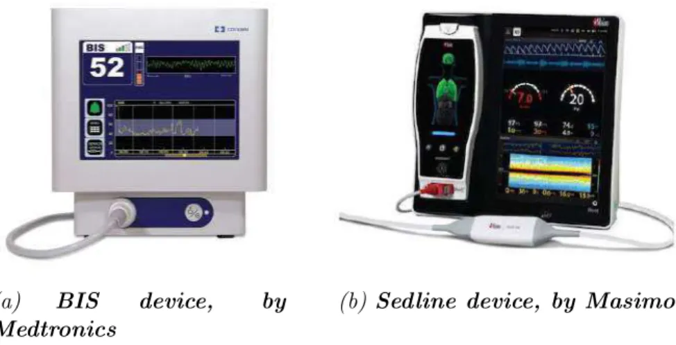
• The Bispectral index (BIS) is an empirically-derived parameter for monitoring depth of anesthesia[LSW96][LSW97], and it is also the name of the Medtronics device used for EEG recording and calculation of this parameter. The original device was introduced in 1994. The BIS index is a continuous index which takes values between 0 (isoelectric EEG) and 100 (awake subject). This value is cal-culated with a weighted sum of several indices including time features, spectral features and bispectral features. Recall that the bispectrum[NR87] of an EEG channel is the two dimensional Fourier transform of its third-order cumulant-generative function: the result is an amplitude as a function of two frequencies. It is a measure of nonlinear couplings in the signal. The BIS is an interesting step towards assistance in the interpretation of EEG, however its validity for monitoring depth of anesthesia is questioned, partly because it is not sensitive to all commonly used anaesthetic drugs[BJOA99][HDBB04], remains sensitive to artifacts. Also, the algorithm for calculating features and the BIS index being proprietary, potential for comparison and improvement is limited.
• The Patient State Index (PSI)[DLP+02] is a another index developed for similar
purposes and associated with a Masimo device. It includes similar features, and the algorithm for obtaining the index is partially disclosed, although the data used for fitting is not.
• Amplitude-integrated EEG[THWG+99] is very simple technique which consists
of viewing peak-to-peak amplitude of a standard EEG over a very compressed timescale, displaying hours to days on a single line. Much information about the shape of waveforms is lost, but a general view is obtained, which helps spot long-term trends in electrical activity for example to inform on seizures or suppressed activity, even for non-trained staff[KOW+11].
• Some EEG review software programs include tools for automatic detection of rather simple items such as spikes, spike-and-waves or bursts of slow-wave activ-ity. However these tools have low specificity and results must be double-checked by the expert. Therefore, little or no time is gained. One notable exception is sleep scoring where automatic interpretation provides reliable help.
(a) BIS device, by Medtronics
(b) Sedline device, by Masimo
Figure 2: Systems using automated interpretation of cEEG for monitoring depth of sedation
Through this brief tour of existing systems it appears that systems for automated analysis of continuous EEGs exist but are still very rudimentary. Given their low specifities, they are only able to provide the clinicians with a ‘red flag’ promoting other diagnosis effort, for example by indicating an EEG recording.
Thesis organization. In summary, several previous works have made clear that cEEG is an rich yet underexploited modality for applications within or beyond the ICU. A goal of this thesis is to improve automated analysis methods for cEEG through the development of more advanced systems which can be taught to ’un-derstand and characterize EEG’. Such improved processing methods an help making better use of cEEG for already-known applications, and hopefully also opening the way to new applications. The remainder of this manuscript is organized as follows:
• In chapter1we introduce how to use machine learning approaches for processing EEG signals and present the available data and some initial experiments.
• Artificial neural networks and deep learning are the main tools we use for building pattern recognition architectures and we introduce them in chapter 2. We then formulate the system envisioned for post-anoxic coma prognostication.
• In chapter3we explore sleep scoring as a first application to validate deep learning methods for pattern recognition on raw EEG signals with supervised learning. • A difficulty with the clinical applications envisioned is that the available
supervi-sion is scarce and ’high-level’. For example for post-anoxic coma prognostication the only reliable supervisory elements are the outcome and the clinical history, no supervision on patterns is easily available. In chapter 4 we present unsupervised methods for learning pattern detectors with little available supervision.
• In chapter 5 we present our findings relating to neural architectures adapted to multichannel EEG and present different modeling possibilities.
5
CHAPTER
1
EEG AND MACHINE LEARNING
Question: What are the possible machine-learning-based approaches towards auto-mated ICU EEG interpretation ? What data can be available to this end ?
Contents
In the previous chapter we explained that we aim at building tools for automated char-acterization of continuous EEG. These tools should pre-analyze, select and summarize EEG tracings in a way that simplifies, complements and enhances the job of the spe-cialist. One possible way to build such systems is to use machine learning, i.e. model the statistical regulatities between groups of EEG signals. In this chapter we start by introducing machine learning and present the available data for our problem. We then give an brief overview on the EEG machine learning litterature and relate to them simple initial experiments.
1.1
Background on EEG and machine learning
1.1.1
Machine learning
The general class of methods that we will use for characterizing EEG content is ma-chine learning methods - also called statistical learning methods. In mama-chine learning, scientists try to develop models that fit statistical regularities of some data and apply these models on unseen data. For example in our case, given many examples (many patients), their features (such as patterns detected in the EEG each hour), and the outcomes, learn a model which predicts the outcome of new (unseen) patients. Learn-ing a model means findLearn-ing a good configuration of its parameters given data and given the prediction task. Machine learning can be broadly categorized into the following subtypes:
1.2. Data 9
Multivariate. An EEG record obviously uses several electrodes spread on the head. Because each electrode has a given spatial position, analysis methods touching upon multivariate analysis will often be called spatial analysis methods. To design spacial analysis methods it is important to understand how cortical sources project on elec-trodes through the conductive medium. A classic and useful model is the forward model which we introduce in Appendix B.
Non-stationarity. An modeling hypothesis described in the forward modelB is that the total signal recorded at each electrode is a (linear) superposition of the electric potential created at this point of space by all active sources. Importantly, sources are non-stationary[KFF+05]. Therefore, the total multivariate signal is also non-stationary.
The time during which it is reasonable to assume that the EEG is stationary depends on the application but the order of magnitude is a second.
Consequences for analysis methods The methods we propose involve detecting or characterizing EEG patterns and then infering something based on these patterns. Since signals are multivariate and non-stationary, methods for detecting all possible patterns are thus spacio-temporal analysis methods. In practice, almost all existing EEG analysis methods include either separate or factorized spacial and temporal anal-ysis - as opposed to hypothetic methods where spacial and temporal analanal-ysis would be performed jointly. For instance:
• Spectral or multispectral power in bands are temporal/frequencial features cal-culated on one channel
• Covariance matrices are spacial features calculated on all channels
• A deep learning pipeline for EEG classification[CGA+17] typically includes a
spacial filtering layer followed by one or more temporal analysis layer
For this thesis we also consider factorized spacial and temporal analysis, i.e. a spacial analysis step followed by a temporal analysis step. This modelisation is probably restrictive though. Extensions of methods from Chapter 5 would be a good starting point for developing methods for joint analysis of spacial and temporal patterns.
1.2
Data
When working on machine learning, the nature, quality and quantity of available data strongly influence the choice of the models. Below we briefly present the available data in our case, for the upper-mentioned application of post-anoxic coma prognostication.
1.2.1
Records performed ourselves
Shortly after the beginning of this PhD work and before having precise ideas about EEG processing methods to be used, we recorded a small number of continuous EEGs on ICU patients with post-anoxic encephalopathy at CHU Grenoble in order to get a grasp of practical aspects of how a recording system can be integrated into the ICU environment, and also check for the classic EEG patterns described in C.2.
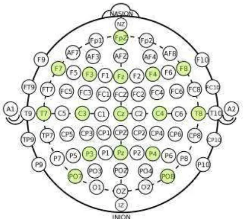
Figure 1.2: Electrode setup used for recordings at CHU Grenoble
Recording hardware We used a g.tec g.USBamp amplifier, conventional cupule elec-trodes, and the Natus-EC2 conductive paste for long-term EEG recordings. We note that this paste also has adhesive properties which help maintaining electrodes. For skin preparation we used Nuprep paste. Electrodes are maintained on the head by a disposable elastic cap. We used 16 electrodes at positions shown on Figure 1.2 and a unipolar montage with mastoid reference and frontal ground. Electrode positions are close to the conventional 10-20 setup but leave the occipital space free so that the patient can comfortably lie on the back of his or her head.
Artifact tagging Upon recording the first patients we noticed that EEG tracings are very sensitive to artifacts. Contaminated tracings can be a problem if the sub-sequent automated processing method is not explicitly designed to handle artifacts. On comatose patients we also noticed that a majority of artifacts correspond to peri-ods when a caregiver is present near the patient or touches the patient. We therefore added a video processing system to the EEG system to perform real-time background segmentation. Is uses the ViBe algorithm[BVD11] and works real-time on the com-puter running the recording software. ViBe works by keeping a (memory-efficient) summary of the distribution of previous pixel values, and updating this summary according to an update scheme. Code for compiling this program can be found at
https://github.com/drasros/motiondetec_eeg_rea.
Obtained data We obtained 10 records from post-anoxic patients. EEG was starting as soon as possible during therapeutic hypothermia and stopped at 48h or before if the condition of the patient was good. Of course such a number of patients is far too small to conduct any machine learning analysis but the recording sessions helped us to get a sense of practical elements. The initial plan was to launch a clinical study and record all post-anoxic patients admitted at CHU Grenoble but we realized that this was an inefficient use of available time.
1.2.2
Records mined from the EEG database at CHU Grenoble
At CHU Grenoble EEGs are recorded routinely on post-anoxic patients as part of stan-dard patient care. These records are almost all short-duration, and performed after
methods have already proven truly successful. Datasets for sleep scoring usually include two channels of raw EEG, along with annotation for sleep stages every 20 to 30 seconds. A very classic dataset is Physionet Sleep-EDFx[GAG+00]. With 61 nights it is rather
small. More recently the Sleep Heart Health Study (SHHS) dataset[QHI+97] became
available, including more than 9000 polysomnographic records (although not all use the same setup).
1.2.5
Summary
To summarize, it is relatively easy to obtain general ICU EEG tracings, also for tracing from post-anoxic coma patients. We emphasize the fact that most of these records are short-duration and performed after rewarming, because continuous EEG during TH is still not very commonly used. For these records High-level annotations can be gathered by going through the medical file. Finally, because of the massive amount of work it represents it is almost impossible to have access reliable annotations including time tags and labels on patterns. This absence of available labels on patterns is the reason why we initially shift from ICU EEG and focus on sleep scoring in chapter3, and then work on unsupervised and semi-supervised methods in chapter 4.
1.3
Possible analysis method and first experiments
In the existing litterature different approaches exist for detecting patterns for EEG machine learning. We give an overview of them below, and briefly present some initial work.
1.3.1
Classic feature extraction
The classic workflow with machine learning on EEG a two step process: first extract features and then use the desired algorithm, for example an SVM or decision tree for classification or a k-means algorithm for clustering. Choosing appropriate feature ex-tractors is very important for performance and this choice involves domain knowledge. We briefly review classic features for EEG. Discussing the range of possible algorithms is beyond the scope of this section. For now, let us consider an EEG epoch (i.e. win-dow) of given length. Methods for extracting features from it include:
Time domain features , for example:
• Statistics of the signal[JPB14] including mean, standard deviation, higher mo-ments, power.
• Shannon entropy[KCAS05] • Non-stationary index[JPB14]
1.3. Possible analysis method and first experiments 13
Frequency and Time-Frequency features are features obtained by spectral de-composition, usually using Fourier or Wavelet transforms. The power in subbands is calculated either on the whole window (frequency decomposition) or on sub-windows (time frequency decomposition). For time-frequency, a balance must be found between frequency resolution and time resolution. Also, a number of methods for estimating the periodogram exist[BB14]. From the power in bands or time-frequency decomposi-tion, other subfeatures can be calculated. Ratios between band power values are often used. Another example is Wavelet subband entropy [ANPZ+03], which consists of performing entropy calculation over the coefficients of the discrete wavelet transform.
Nonlinear features can also be used. These include for example complexity mea-sures such as the Kolmogorov-Chaitin complexity[SKEK+14] and higher-order
spec-tra[Nik93].
Cross-channel features are used for different applications amongst which Brain-Computer interfaces(BCI). For such applications, the classes to be separated usually have different spacial signatures. For example, in motor imagery the zone of the cortex associated with imagining to move the hand is different than the zone associated with imagining to move the foot. Therefore electrical signatures have different spacial sig-natures. Cross-channel features are also interesting for ICU EEG. For example in ICU EEG epileptiform patterns often involve synchronized patterns spread over a zone. A typical cross-channel feature is the spacial covariance matrix. Note that the space of covariance matrices is the ensemble of symmetric positive definie matrices. This space has a particular geometry, and it is avantageous to draw the connection to Riemannian geometry[BBCJ13].
1.3.2
Design of application-specific pattern detectors
The previous subsection introduced an number of features classically used on EEG for machine learning. For the case of ICU EEG, rather than using such features, another possible approach is to explicitly design detectors for the clinical patterns known to be of interest. The rationale behind such approaches is to take an intermediate step between fully-visual and fully-automated interpretation, and allow simple clinical studies on linking typical patterns to clinical predictions.
Below we describe possible methods for devising such pattern detectors, for the typical ICU EEG patterns introduced in C.2.
Isoelectric or low voltage signals are relatively easy to detect with simple amplitude criteria and thresholds.
Diffuse slowing can be characterized with spectral analysis, for example using ratios of power in slow versus high frequency band.
4 5 6 7 8 9 10 11 12 −200 −100 0 100 200 time (s) amplitude (microV)
(a)example single-channel segment of a record showing epileptiform patterns
0 10 20 30 40 −20 0 20 40 Frequency (Hz) DSP (d B )
(b)multitapered periodogram on this segment
600 650 700 750 800 0 10 20 30 40 time (s) F requency (Hz) −40 −20 0 20 DS P (d B )
(c) 200 second spectrogram calculated on the same record using a multitapered periodogram
Figure 1.4: Examples of spectral analysis on an EEG channel from a record showing generalized periodic epileptiform discharges. Here periodograms are calculated using the multitaper method[BB14].
0 1 2 3 4 5 6 time(s) −1.0 −0.50.0 0.5 1.0 no rm ali ze d am pli tud e EEG signal segmentation
(a) 6-second segment with short and frequent bursts. Segmentation parameters: β = 0.9633 and vmax= 75 0 5 10 15 20 time(s) −1.0 −0.50.0 0.5 1.0 no rm ali ze d am pli tud e EEG signal segmentation
(b) 20-second segment with longer and more spaced bursts. Segmentation param-eters: β = 0.9633 and vmax = 150
Figure 1.6: Segmentation of records with burst-suppression
1.3.3
Learned feature extractors
A last possible approach for characterizing EEG patterns is to learn feature extractors. In other subfields concerned with characterizing continuous signals the classic way to do this is to use deep neural networks trained end to end. For most applications such deep learning methods have proved superior to classical approaches[LBH15], however they are not an answer per se to the question of how to deal with (the lack of) annotations. In the following of this thesis we focus on such methods and develop further.
1.3.4
Summary of possible pattern characterization methods
In summary, we exposed three possible approaches for automatically characterizing EEG content. For us focusing on feature engineering makes little sense because no an-notations are available and therefore no reliable way of measuring progress stands out. The second approach of building detectors aimed at detecting standard patterns (as in the standard ICU EEG terminology[HLG+13]) has the same problem with annotation
and additionally, ‘real-life’ patterns include not only ‘textbook’ patterns but also many intermediate patterns between which humans are able to subjectively interpolate using experience rather than hard-coded rules. We advocate that training automated algo-rithms to reproduce such categories is acceptable only for ’proof-of-concept’ studies, and that proper automated characterization should leverage the possibilities of ma-chine learning algorithms rather than reproduce (in a worst version) human analysis. Given the above, we propose to focus our work on the third approach. We propose to develop and evaluate deep learning methods on EEG analysis. We emphasize that such methods are not an answer to a lack of annotations, but we will present ways in which they can be used in semi-supervised settings to try to compensate for this.
1.3. Possible analysis method and first experiments 17
Summary of the chapter:
• We formulated how machine learning can be used for EEG characterization. • We introduced available data. We explained that the envisioned applications are
difficult because they are weakly supervised.
• In the rest of the thesis we focus on methodological developments. We are not able to address a full application such as post-anoxic coma prognostication because we do not have labels.
CHAPTER
2
ARTIFICIAL NEURAL NETWORKS
Question: What are artificial neural neworks and how can they help for EEG pattern characterization ?
Contents
1.1 Background on EEG and machine learning . . . 8 1.1.1 Machine learning . . . 8 1.1.2 EEG specificities . . . 9 1.2 Data . . . 10 1.2.1 Records performed ourselves . . . 10 1.2.2 Records mined from the EEG database at CHU Grenoble . . 11 1.2.3 Other sources of ICU data . . . 12 1.2.4 Non-ICU data . . . 12 1.2.5 Summary . . . 12 1.3 Possible analysis method and first experiments . . . 12 1.3.1 Classic feature extraction . . . 13 1.3.2 Design of application-specific pattern detectors . . . 15 1.3.3 Learned feature extractors . . . 16 1.3.4 Summary of possible pattern characterization methods . . . . 17
Artificial neural networks (ANNs) are machine learning models used for approximat-ing complex mappapproximat-ings, often from a high-dimensional space (signal space) to a low-dimensional space (label space). In practice, such mappings correspond for example to a regression function or a classifier. ANNs are often used with raw samples of nu-merical signals (coming from continuous modalities) as input, such as pixel values in images, or sample values in speech or EEG. The main techniques behind ANNs date
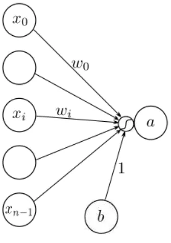
Figure 2.1: A single artificial neuron, represented with input values, weights, bias and activation function.
back to the nineties or even before, but practical success of deep learning only took place from 2012 when larger datasets and adequate computational resources became available[KSH12]. In the last five years ANNs have brought spectacular advances in processing images and videos, text, speech and audio signals[LBH15], and also when combined with reinforcement learning[SSS+17].
2.1
Basics
The artificial neuron is the basic building block of ANNs. As shown on Figure2.1, it uses weights w and a bias b on input x to perform the computation xout = f (w⊺x+ b).
The function f (.) is a non-linear activation function such as a sigmoid, hyperbolic tangent, or rectified linear unit. A single artificial neuron implements a linear separator.
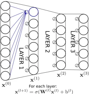
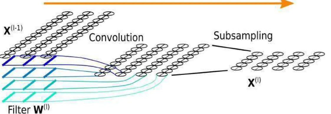
Multilayer systems. Deep neural networks are usually built by stacking layers of articifial neurons. The input and output of a layer are groups of scalar values. A layer represents the operation performed to obtain output values from input values, for example a matrix multiplication followed by a pointwise non-linearity. The first layer typically takes raw samples as input, for example EEG samples on a single-channel segment. For following layers the input values are output values from the last layer. An ANN is the ensemble of its layers. The process of calculating the ouput of the ANN from its input is called forward propagation. Artificial neural networks with several layers are called deep neural networks, hence the denomination deep learning. Figure
2.2shows a three-layer ANN. Layers that are not input or output layers are often called hidden layers.
Why do multiple layers help? In practice what we want to use ANNs for is ap-proximating complex non-linear mappings, for example to predict the content of an image amongst a number of possible labels, or discriminate epileptiform patterns in EEG. We want do so with systems using as few parameters as possible, in order to require fewer training data and perform better in the bias/variance tradeoff. Multilayer
2.1. Basics 21 L A Y E R 1 L A Y E R 2 L A Y E R 3
For each layer:
Figure 2.2: Diagram showing a network with 3 stacked layers. Units (or neurons) are circles. A layer represents the operation to obtain a set of activations x(l+1) from the previous set of activations x(1). σ denotes a non-linear function applied element-wise. In fully-connected layers each neuron is connected to all values from the previous layer, as shown with the blue neuron.
systems help because they can fit more more complex functions with fewer parameters. Appendix E provides an intuitive explanation on why this might be the case. It was shown [HSW89] in 1989 that multilayer fully-connected neural networks are universal approximators, meaning that in theory any measurable function can be approximated to any desired degree of accuracy by a two-layer neural network with sufficient number of hidden neurons. This, however does not tell how large the number of hidden neurons should be and how to train such a network. In practice, for keeping the total number of parameters reasonable and avoiding overfitting, two things help: more depth, i.e. more (smaller) stacked layer, and different neural architectures to improve on the simple fully-connected layer.
Last layer activation In practice, an ANN is designed to approximate some map-ping. Depending on this mapping, is expected to produce outputs of a certain type (for example, binary vs. continous, univariate vs. multivariate) and in a certain range. For example, a classification task requires categorical outputs. It is thus necessary to adapt the activation function of the last layer to the targeted application: for example for regression with targets in R a linear activation function can be used. For binary classification, sigmoid activations are appropriate for generating outputs in [0, 1] that can be interpreted as the probabilities of each prediction to be true. For classification tasks, the softmax activation function[Dun] is classic. It consists of exponential activa-tions normalized so that output values can be interpreted as class probabilities. With j the class number and z the values of the output layer before the activation function, the output units of the softmax activation xsof tmax take the form:
xsof tmaxj = e
zj
P
kezk
2.2
Standard architectures
We presented neural layers as mathematical operations to transform a set input values into a set of output values. In fully-connected layers each neuron takes all input values of the layer for its own input. In practice, many other layer architectures exist. For a given problem, an optimal architecture is one that is able to fit the desired input-output function while using the least parameters. For example, convolutional architectures are well-suited to the multiscale structure of images, while recurrent architectures are good for sequencial problems such as automatic translation.
2.2.1
Convolutional layers
Convolutional layers were originally introduced for digit recognition[LBD+90]. Today
still, they are mainly used on images. Below we briefly present the different types of convolutional layers. Images involve 2D convolutions whereas EEG involves 1D (tem-poral) convolution. We believe that it is better to present convolutional layers using 2D convolution (and we do so below) because (1) it better relates to computer vision litterature - from which almost all research originates from - and to practical imple-mentation frameworks (2) it will happen in the chapter on multichannel architectures (5) that we ‘hack’ a 2d convolution to perform some filtering operation and (3) all of our practical implementations are based on adaptations of 2D convolution layers. Convolutional layers perform several convolution operations on several sub-parts of the input using several different filters. In computer vision research papers the term ‘convolution’ is often used interchangeably for a convolution operation, a convolution layer, of even an ‘assembled layer’ including convolution and subsampling, or more complex things. This can be misleading. Below we describe and distinguish between the convolution operator (and its variants), the various ways in which such operations can be assembled into convolutional layers, and some classical ‘higher level’ assembled layers.
The convolution operation. Let us consider a 2D input signal X ∈ RhX×wX and
a convolution kernel K ∈ RhK×wK. Convolving the kernel on the input consists in
‘sliding’ it onto the input and performing element-wise multiplication and sum for each position (Note: Strictly speaking, this form corresponds to a cross-correlation rather than a convolution, or in other words convolution with a flipped kernel. For deep learning where filters are learned this has no importance). The result of convolving X with K is: S(i, j) = (X∗ K)(i, j) = hK X l=0 wK X m=0 X(i + l, j + m)K(l, m) (2.2)
where hx, wx denote the height and width of the input, hk, wk the height and width
of the kernel.
On top of this base definition, a convolution operation as used in ANNs needs other characteristics to be fully defined. We briefly list and illustrate them below. Graphics
2.2. Standard architectures 25 convolution operations convolution operations sum along depth sum along depth concatenate
Figure 2.7: A standard convolution layer with four input feature maps (cX = 2) and two output feature maps (cX˜ = 2).
convolution operations using same filter on all input feature maps
concatenate
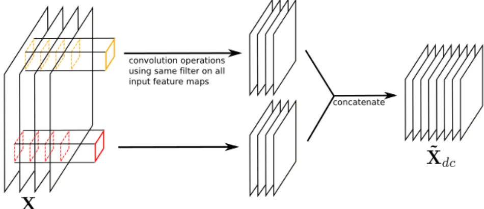
Figure 2.8: A depthwise convolution layer, here represented with cX = 4 replicated filters and αc = 2.
filters (as the red and orange columns on Figure ??) where each filter is applied on one channel only. The depthwise convolution layer in its original formulation (and also in the reference Tensorflow API for example) actually does not do that and is slightly more general. It simply consists of a standard convolution where depthwise summation is not performed. Using similar notations, where input X has shape [hX, wX, cX], filters K have shape [hK, wK, cX, αc] where αc ∈ N∗+ is a
channel multiplier, and output ˜Xdc has shape [hX˜, wX˜, cXαc], we have:
˜
Xdc[:, :, αr + q] = X[:, :, q]∗ K[:, :, q, r] (2.4)
The term ‘depthwise convolution’ starts to make sense when each of the αc filters
is applied on all cX input channels (or in other words, the filter tensor K contains
cX identical replicated filters of shape [hK, wK, αc]). This is usually what is done
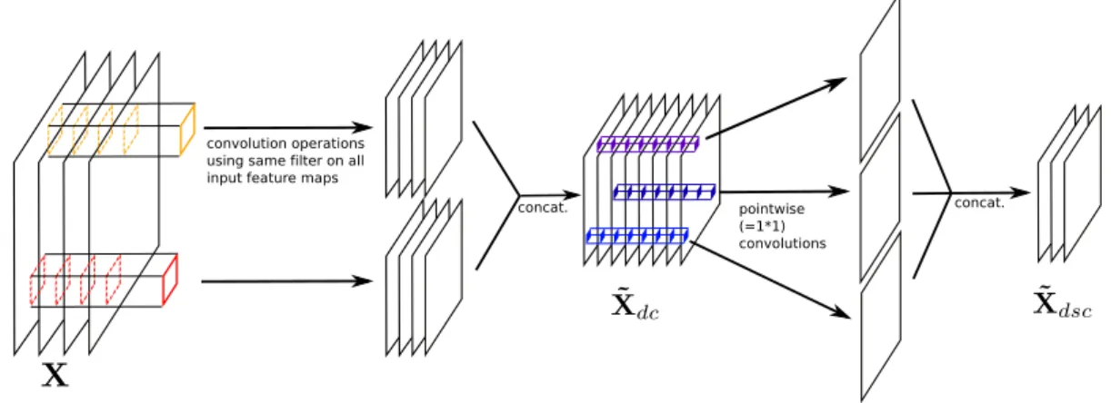
in papers claiming to use depthwise convolution layers (or depthwise separable convolution layers)[KGC17]. Figure 2.8 shows a depthwise convolution.
• Depthwise separable convolution layers are another type of convolution layer that we use in 5. Also abbreviated separable convolutions, they consist of a depth-wise convolution followed by a pointdepth-wise convolution. A pointdepth-wise convolution is one way to note a linear recombination of output feature maps. Still using the same notations, input X has shape [hX, wX, cX], depthwise filters K have shape
convolution operations using same filter on all input feature maps
concat. pointwise concat. (=1*1)
convolutions
Figure 2.9: A depthwise separable convolution layer, here represented with cX = 4 replicated filters, αc = 2 and cX˜ = 3.
[hK, wK, cX, αc], pointwise filters Kp have shape [1, 1, cXαc, cX˜] and output ˜Xdsc
has shape [hX˜, wX˜, cX˜]. The expression of the output is:
˜ Xdsc[:, :, s] = X q ˜ Xdc[:, :, q]∗ Kp[0, 0, q, s] (2.5)
Figure 2.9 shows a depthwise separable convolution.
• Note that other types of convolutional layers exist, for example to target efficiency and minimal number of operations on mobile devices[HZC+17][ZZLS17]. For now
we are not concerned with these.
Classic convolution-based modules. As mentionned before, convolutions are of-ten used jointly with pooling or strides. Other ‘higher-level’ assembled modules on convolutional layers exist that have become relatively standard in the implementation of Convolutional Neural Networks (CNNs), for example:
• Inception layers are a type of assembly that lets the model ‘choose’ between different sizes of filters. It was first implemented in Google LeNet[SLJ+15] and
was since then decline in variants, building on the fact that large filters can be implemented using less parameters by two (or more) hooked one behind each other[SVI+16][Cho16][KGC17]. Figure 2.10 shows an Inception layer.
• Residual layers[HZRS16] were introduced as the solution to the fact that increas-ing depth of CNNs often helps, until the networks are too deep to optimize usincreas-ing gradient descent due to problems related to gradient flow. In a classical convo-lutional layer, the layer learns a mapping. In a Residual Network (ResNet), the convolutional part of each layer learns the difference between this mapping and the identity function. This way, if the network is in a configuration where it is too deep, the layer can just remain the identify function and not break gradient flow. Figure 2.11 shows a residual layer. We use residual connections in architectures from 5.
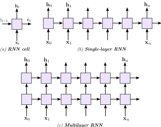
(a) RNN cell (b)Single-layer RNN
(c) Multilayer RNN
Figure 2.12: An RNN consists of recurrently applying an RNN cell to the values in a sequencial input
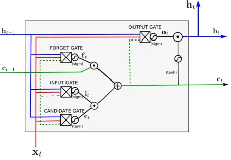
2.3. Optimization 29 FORGET GATE INPUT GATE (sigm) (sigm) (tanh) CANDIDATE GATE (sigm) OUTPUT GATE (tanh)
Figure 2.13: An LSTM cell. xt denotes the input vector at step t, ct the cell internal state at step t, and ht the output for step t.
and next state are obtained by simple matrix multiplication from the current input and previous state. A much more used cell is the Long Short-Term Memory (LSTM) cell[HS97]. It addresses the main weakness of the simple RNN cell, which is to kill gradient flow on long sequences. It does so by adding some gates that allow the propagation of ‘memories’ over longer ranges. Figure ?? shows an LSTM cell. A number of other types of RNN cells and architectural developments exist. Two classic other developments are attention[BCB14][VSP+17] and explicit memory[SWF+15].
RNNs are good on sequences with reasonable length, for example dozen to hundreds of samples. Beyond that, it is difficult to learn long-term dependencies in temporal patterns because backpropagation (see next section) through that many steps becomes computationally costly and less stable. This is why the flagship application for RNN is automatic translation (text to text). On audio signals it is usually suitable to work from time-frequency features or some convolutional features. In terms of how many samples a typical pattern covers, EEG lies somewhat inbetween text and speech. Our work with RNN on EEG has only been preliminary and the best means of using them remain to be developed. Note that of course RNNs can be combined with CNNs in models.
2.3
Optimization
So far we have seen how to use different types of architectures to build ANNs. An ANN transforms an input to an output using connections of mathematical layers interspersed with non-linear functions. Each layer has a number of parameter weights. To do anything useful, the network has to have its weights in a good configuration. Starting from random values, optimization consists in finding adequate values for the weights, given a set of training examples and given a task for the network.
2.3.1
Cost functions
The cost function - also called loss function - is a metric used to quantify how close current neural network outputs are from the target values. For example, for a classifi-cation task with softmax activation on the last layer (also called softmax regression), cross-entropy is often used as a cost function. Let xin be a training example and t be
the one-hot encoded target class (i.e. a vector with zeros everywhere except on the position of the target class) for this training example. Let w the vector of all trainable parameters and xout be the output activation. The cross entropy cost is a
multidimen-sional generalization of the logistic regression cost, and for one example it takes the form:
l(xin, w) =
−t log xout(xin, w) (2.6)
Minimizing this cost averaged on test set examples corresponds to maximizing the log probability of the model-predicted class being equal to the true class. Depending on the application other cost functions can also be used, from simple costs such as squared error for regression to more advanced ones such as adversarial losses for unsupervised learning.
2.3.2
Optimization
Gradient descent. Optimization of weight values is done by first or second order stochastic optimization - most of the time gradient-based optimization. The loss l(x, w) can be calculated and averaged on all examples from the training setT . The resulting loss l(w,T ) is a differentiable function of weights w. The basic optimization algorithm is iterative. One step of it consists in calculating all derivatives and updating weights in the direction of the ‘downhill gradient’:
wt= wt−1− η∇wl(wt−1,T ) (2.7)
where η is called the learning rate. Gradients are estimated using error backpropa-gation. Error backpropagation is behind pretty much all optimization algorithms for deep learning today. It is described in further detail in Appendix F. This iterative process is repeated until convergence.
Weight initialization As seen in the above paragraph optimization methods for find-ing good values for the weights iterative. Therefore, before startfind-ing the optimization process weights need to be given initial values. A number of initialization strategies exist. Which one to use is linked to the type of normalization strategies and nonlin-earities chosen. The basic principle for designing them is keep the activation of layers (mean and standard deviation of output neuron numerical values) constant within the successive layers. For example, the classic Xavier initialization[GB10] scheme con-sists in initializing weights of a layer in U [−√ √6
nin+nout,
√ 6 √n
in+nout] where nin an nout are
the numbers of input and output neurons. It is adapted for networks with sigmoidal activations. Other techniques exist, such as the He normal initializer[HZRS15] for
2.3. Optimization 31
Rectified linear units (ReLU) or orthogonal random matrix initialization[SMG13] for encouraging uncorrelated activations in a layer.
Stochastic optimization. Estimating gradients ∇wl(w,T ) on the whole training
set is very costly. For each optimization step a forward pass and a backward pass on each training example must be done. For big datasets this quickly becomes unfeasible. Stochastic optimization consists in estimating gradients ∇wl(w,B) on minibatches B
of a small number of examples rather than on the whole training set, and uses such esti-mates for weight updates. This allows much faster estiesti-mates which can be statistically almost as good and also leverage the parralelisation capabilities of modern hardware (GPUs). A whole subfield is concerned with studying such algoritms.
Training algorithms. Simple gradient descent consists of steps in the gradient di-rection. The multidimensional loss surface can have complex shapes and this simple strategy is not always the most effective.
• Momentum is a first improvement that helps escaping low slope regions and avoiding oscillating gradients in regions where isoenergy surfaces are very ‘non-circular’. Momentum consists of updating parameters in the direction of accu-mulated gradients:
vt = γvt−1+ η∇wl(wt−1,B) (2.8)
wt = w(t−1)− vt (2.9)
γ is the momentum and is usually chosen at about 0.9. It can be lower than this at the beginning of optimization to encourage gradient variance, and be decreased after a few sweeps through the training set. Momentum also exists with the Nesterov momentum variant which consists of anticipating energy surface shape change by evaluating the gradient near the ‘next position’ rather than current position.
• Adaptive learning rate algorithms are another interesting improvement to the learning rule. Such algorithms use adaptive learning rates per parameter. One learning rate per parameter allows to perform larger updates for the most infre-quently updated parameters. Adaptive means that a memory of the norms of past gradients is kept for each parameter and used to scale the current learning rate.
Adaptive learning rate algorithms come in several flavors: Adagrad[DHS11], Adadelta[Zei12], RMSProp, Adam[KB14a]. The most recently introduced (and widely used) is Adam. It works well on sparse gradients and naturally performs a form of step size annealing during training.
• Finally, some authors have experimented with second order methods[Mar10]. These take into account also cost function curvature. Second order methods are far less explored than first order ones as they are more complex. The difficult
question is how to estimate the update step given curvature information. Calcu-lating the full Hessian matrix is generally not feasible. Solutions involve either ap-proximating the Hessian matrix - for example L-BFGS[LN89] does this - or avoid-ing Hessian computation - for example usavoid-ing Hessian Free Optimization[Mar10] or Kronecker-factored approximate curvature[MG15b].
Regularization A well-trained model should generalize well, i.e. perform well on test examples that it has not been trained on. Poor generalization occurs when the model overfits the training set. Overfitting occurs in cases when the model has too many parameters for the number of training examples and complexity of the data. For a given model, Regularization methods help avoiding overfitting:
• Getting more data is almost always the best approach if the model overfits. In practice this is not always possible. The other approach consists of limiting model capacity, which can be done in several ways:
• Early stopping consists of monitoring performance metrics on a validation set during training, and stoppping training when these validation metrics stop im-proving.
• Weight decay consists of penalizing large weight values, for example with an L2-norm penalty.
• Addition of noise to the weights or the activities also has an important
regulariza-tion effect. Noise was originally used on the input, as in denoising autoencoders[VLL+10].
However it can also be used on an entire network: the classic example is Dropout[SHK+14].
Dropout consists in setting a certain fraction of the activities to zero randomly during each forward pass.
• Batch normalization[IS15] consists of normalizing layer activities for each train-ing mini-batch. This has the effect of stabiliztrain-ing the distribution of the inputs to the next layer - avoiding the internal covariate shift phenomenon - and allowing higher learning rates. Batch normalization also has the (experimentally con-firmed) effect of regularizing the model, although the theoritical reasons behind this are not very well understood.
Algorithm 1: Batch normalizing transform, applied to ac-tivation x over a mini-batch. From [IS15]. Note that in practice a moving average of µB and σB is kept.
input : values of activation x over a mini-batch: B = {x1..m}, Scaling parameters γ, β (learned)
output : yi = BNγ,β(xi)
µB ← 1 m
Pm
i=1xi // mini-batch mean
σ2 B ← m1
Pm
i=1(xi− µB)2 //mini-batch variance
ˆ
xi = √xi−µB σ2
B+ǫ
//normalize
2.4. Brief review: EEG and deep learning 33
• Layer normalization[BKH16] uses a similar idea but normalization is performed along units of a same layer rather than along examples of a same batch for each unit. It is more straightforward to use because it performs the same computation at training an test times, using no moving average. It is useful for recurrent networks.
• Finally, weight normalization[SK16] consists of explicitly decoupling the norm and direction of weight vectors in neural layers, using the parameterization w =
g
||v||v. Similarly to layer normalization, weight normalization does not introduce
dependencies between the examples in a mini-batch. It allows similar speed-ups to normalization with lower overhead. However, for best performance it requires data-dependent initialization - this is a little tricky and has slowed down its adoption. Weight normalization works best with CNNs.
2.3.3
Practical implementation tools
A number of frameworks exist from implementing ANNs. The most popular ones are Theano, Tensorflow, Torch/pyTorch and Caffe. The main interest of using such frame-works is twofold. First, such libraries allow symbolic differentiation which considerably simplifies training compared to calculating and checking gradients manually. Second, these libraries offer the possibility to run calculations on a Graphical Processing Unit (GPU) in a way that is almost transparent to the user. Parralelization takes effect both at batch level and operator level. This speeds up training notably. In our case, we started our work using Theano[The16] and switched to Tensorflow [AAB+16]
af-terwards. Both of these libraries use computational graphs defined statically (unlike Torch and Pytorch where graphs are defined dynamically at execution time). They are written with a Python API over a C/C++ and CUDA engine. Most of our models are trained on an Intel workstation equiped with an Nvidia GTX-980Ti GPU.
2.4
Brief review: EEG and deep learning
ANNs and deep learning are old techniques whose applicative success is relatively recent (from 2013). Their use on EEG signals is relatively scarce although it seems to have significantly taken off in the last year. To link the afore-presented techniques to EEG, we give a brief tour of the most significant existing work using deep learning on EEG time series, for various applications not limited to ICU.
2.4.1
With preprocessed input
Until approximately late 2016, all existing work on EEG and deep learning was con-cerned with using neural networks as classifiers on features classically extracted from EEG signals.
• The authors of [MLMK08] use bivariate features calculated on 5-second windows of EEG from patients prone to epilepsy, aggregate features from 1 to 5 minute
2.5
Automated interpretation of ICU EEG: envisioned
solution
Question: How to build a method that combines the fine pattern characterization ca-pabilities of ANNs on short patterns with the ability to analyse EEG content evolution over long sequences for leveraging continuous EEG ?
Now that we have briefly presented ANNs and most relevant works applying them on EEG, we describe the ‘global’ solution envisionned for adressing an ICU application. On applications presented in [ADD CH], the machine learning task requires analysing local patterns and their variations over time - where ‘local’ represents the typical pat-tern duration (or basic unit of time), and ‘variations’ can span anything from a few units of time to several hours.
Such applications are challenging because inputs have very high dimensions and because the number of labels is small in comparison to ‘standard’ machine learning tasks. For example, a standard image classification problem addressed with neural networks can use 64× 64 × 3 inputs, i.e. 12288 dimensions, and the models will be trained using at tens of thousands of labels. In our case, a day of 19-channel EEG resampled at 64 Hz represents more than 100 million scalar values - or 4 orders of magnitude higher than the afore-introduced image, and a typical middle-scale clinical study could provide in the order of one thousand labels. Additional labels on short patterns are not easily available. This imbalance hints to the fact that it will probably not be possible to address clinical applications with a unique feedforward model working on the full EEG sequence and trained in a fully supervised manner.
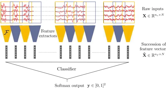
As introduced in 2.4.2, the authors of [vPHRTC17] simply choose to abandon char-acterizing the temporal dynamics and simply train a classifier to predict the outcome from short windows chosen around a given time in the sequence. This already gives good results, but it is probably possible to go further and better exploit continuous EEG. Figure 2.16 provides a representation of a possible pipeline for predicting the outcome of post-anoxic coma from continuous EEG. We detail it below. Note that by using similar feature extractors but replacing the classifier by something else, other applications could be addressed.
2.5. Automated interpretation of ICU EEG: envisioned solution 37
Figure 2.16: A representation of the envisioned contruction for estimating the out-come of post-anoxic coma from continuous EEG.
Each input signal is a multivariate time series X ∈ Rnc×N. Classification happens in
two substeps. In the first step, the EEG sequence is transformed in a time series of feature vectors ˜X ∈ ∈Rnf×N, where feature extractors perform pattern
characteriza-tion. Feature extractors can work on successive EEG epochs (windows) and perform the same operation for each epoch. In the second step, a classifier predicts the outcome from the series of feature vectors. Note that:
• Feature extractors can be fixed in advance (classical features) or learned. As exposed in1.3.4, we choose to use learned feature detectors based on deep neural networks. The neural networks have shared weights, or in other words, the same network is applied to all epochs. However, for reasons detailed above it will probably not be possible to train this network from scratch using supervised learning on outcome labels only. This is why we propose to use unsupervised learning for pretraining. Chapter 4presents our work on this topic.
• Which classifier to use to the subsequent applicative step is beyond the scope of this manuscript. Working on this step will necessitate adequate data and labels. A simple subsampling RNN and softmax regression layer will probably do the job.
• A number of ways to train the full model with semi-supervised learning are pos-sible:
⋆ learn the feature extractor in an unsupervised manner first, then learn the classifier using labels
⋆ learn the feature extractor in an unsupervised manner first, then learn the classifier using labels, while fine-tuning the feature extractor end-to-end at the same time
⋆ learn both at the same time using a multitask-learning scheme with a loss function combining a supervised and an unsupervised loss
• We introduced feature extraction using the notion of successive epochs. It is understood that the extraction can also be ‘progressive’ , using convolutions or recurrent steps together with subsamping steps.
For the following of the thesis we suppose that the end-problem will be addressed as exposed above, and focus on developing the required elements for such a solution. Chapter 3 evaluates the possibility of using CNNs as feature extractors on raw EEG, and does so in a supervised manner. In chapter4some unsupervised techniques for un-supervised learning using ANNs are developed. Finally, in chapter5some architectures for multichannel analysis are devised.
Summary of the chapter:
• We introduced neural layers in various architectures and how to assemble them into multilayer systems (deep networks).
• We introduced basic cost functions, backpropagation and optimization methods for training the networks.
• We envisioned a solution for applying deep neural networks to continuous EEG tasks.
CHAPTER
3
SLEEP SCORING FROM EEG USING
CONVOLUTIONAL NEURAL NETWORKS
Question: Can we prove on a simple supervised application that ANNs on raw EEG signals make sense for characterizing EEG patterns ?
Contents
2.1 Basics . . . 20 2.2 Standard architectures . . . 22 2.2.1 Convolutional layers . . . 22 2.2.2 Recurrent networks . . . 27 2.3 Optimization . . . 29 2.3.1 Cost functions . . . 30 2.3.2 Optimization . . . 30 2.3.3 Practical implementation tools . . . 33 2.4 Brief review: EEG and deep learning . . . 33 2.4.1 With preprocessed input . . . 33 2.4.2 On raw EEG signal . . . 34 2.5 Automated interpretation of ICU EEG: envisioned solution 36We stated above why we want to use ANNs for analysing EEG patterns. As briefly reviewed in chapter 2.4, at the time when we started working on deep neural net-works for EEG and until quite recently, no work using ANNs on raw EEG had been published. Challenging the classical paradigm of analysing EEG from time-frequency representations was not completely obvious. Before diving into more complex analysis method involving multichannel and unsupervised methods, we deemed it necessary to first evaluate a classical deep learning pipeline on a simple supervised prediction task.
Sleep scoring, as a classic application of automated EEG analysis with multiple open datasets available, seemed a good task for doing so. We adapted a 1D-CNN for sleep stage prediction, providing in the meantime notions on which architectural parameters (kernel size, subsampling...) are adapted for EEG. The rest of this chapter is from the article A convolutional neural network for sleep stage scoring from raw single-channel EEG, accepted for publication in Biosignal Processing and Control.
3.1
Abstract
We present a novel method for automatic sleep scoring based on single-channel EEG. We introduce the use of a deep Convolutional Neural Network (CNN) on raw EEG samples for supervised learning of 5-class sleep stage prediction. The network has 14 layers, takes as input the 30-second epoch to be classified as well as two preceding epochs and one following epoch for temporal context, and requires no signal prepro-cessing or feature extraction phase. We train and evaluate our system using data from the Sleep Heart Health Study (SHHS), a large multi-center cohort study including expert-rated polysomnographic records. Performance metrics reach the state of the art, with accuracy of 0.87 and Cohen kappa of 0.81. The use of a large cohort with multiple expert raters guarantees good generalization. Finally, we present a method for visualizing class-wise patterns learned by the network.
3.2
Introduction
Sleep is an essential ingredient for good human health. A number of sleep disorders ex-ist, among which insomnias, hypersomnias, sleep-related breathing disorders, circadian rhythm sleep-wake disorders, parasomnias, sleep movement disorders. Polysomnogra-phy (PSG) is the main tool for diagnosing, following, or ruling out sleep disorders. A polysomnogram is a collection of various signals useful for monitoring the sleep of an individual. It uses physiological signals (EEG, EMG) and environmental signals (mi-crophone, accelerometer). Sleep staging consists of dividing a polysomnographic record into short successive epochs of 20 or 30 seconds, and classifying each of these epochs into one sleep stage amongst a number of candidate ones, according to standardized classification rules[Rec71][BBG+12]. Sleep staging can be carried out either on a whole
polysomnogram or on a subset of its channels, and either by a trained expert or by an algorithm. In some cases the expert can use an algorithm for pre-scoring. The suc-cessive representation of sleep stages over the night is called a hypnogram. It provides a simple representation of the sleep which is useful for suspecting or diagnosing sleep disorders. Sleep staging is a tedious task which requires considerable work by human experts. Also, the quality of the rating depends on the experience and fatigue of the rater and inter-rater agreement is often less than 90%[SLP+13][WLKK15]. Hence the
demand for automated sleep staging algorithms.
In this article, we consider single-channel EEG sleep staging. Whilst it constitutes a first step towards multichannel analysis systems, single-channel sleep staging is also