HAL Id: hal-01819588
https://hal.archives-ouvertes.fr/hal-01819588
Submitted on 20 Jun 2018
HAL is a multi-disciplinary open access
archive for the deposit and dissemination of
sci-entific research documents, whether they are
pub-lished or not. The documents may come from
teaching and research institutions in France or
abroad, or from public or private research centers.
L’archive ouverte pluridisciplinaire HAL, est
destinée au dépôt et à la diffusion de documents
scientifiques de niveau recherche, publiés ou non,
émanant des établissements d’enseignement et de
recherche français ou étrangers, des laboratoires
publics ou privés.
Quality Assessment of Deep-Learning-Based Image
Compression
Giuseppe Valenzise, Andrei Purica, Vedad Hulusic, Marco Cagnazzo
To cite this version:
Giuseppe Valenzise, Andrei Purica, Vedad Hulusic, Marco Cagnazzo. Quality Assessment of
Deep-Learning-Based Image Compression. Multimedia Signal Processing, Aug 2018, Vancouver, Canada.
�hal-01819588�
Quality Assessment of Deep-Learning-Based Image
Compression
Giuseppe Valenzise∗, Andrei Purica†, Vedad Hulusic‡, Marco Cagnazzo†
∗L2S, UMR 8506, CNRS - CentraleSupelec - Universit´e Paris-Sud, 91192 Gif-sur-Yvette, France †LTCI, Telecom ParisTech, 75013 Paris, France
‡Department of Creative Technology, Faculty of Science and Technology, Bournemouth University, UK
Abstract—Image compression standards rely on predictive
cod-ing, transform codcod-ing, quantization and entropy codcod-ing, in order to achieve high compression performance. Very recently, deep generative models have been used to optimize or replace some of these operations, with very promising results. However, so far no systematic and independent study of the coding performance of these algorithms has been carried out. In this paper, for the first time, we conduct a subjective evaluation of two recent deep-learning-based image compression algorithms, comparing them to JPEG 2000 and to the recent BPG image codec based on HEVC Intra. We found that compression approaches based on deep auto-encoders can achieve coding performance higher than JPEG 2000, and sometimes as good as BPG. We also show experimentally that the PSNR metric is to be avoided when evaluating the visual quality of deep-learning-based methods, as their artifacts have different characteristics from those of DCT or wavelet-based codecs. In particular, images compressed at low bitrate appear more natural than JPEG 2000 coded pictures, according to a no-reference naturalness measure. Our study indicates that deep generative models are likely to bring huge innovation into the video coding arena in the coming years.
I. INTRODUCTION
Current image compression methods rely substantially on transform coding: instead of searching for an optimal vector quantizer in the pixel domain, which is a hard problem [1], they transform the input data into an alternative representation, where dependencies among pixels are greatly reduced and an ensemble of independent scalar quantizers can be used. A proper choice of the transformed domain is fundamental to compact the energy of the signal into a few coefficients, and to enable perceptual scaling. Traditionally, image compression standards have been mainly employing linear representations, such as the discrete cosine transform (DCT) [2], used in block-based coding algorithms such as JPEG and in video codecs such as H.264/AVC and HEVC, as well as wavelet transforms [3], used in JPEG 2000. These representations are optimal only under strong assumptions about the underlying distribution of image data, e.g., local stationarity, smoothness or piece-wise smoothness. Failure to meet these assumptions is the cause of typical visual artifacts, such as ringing and blur. More recent techniques, such as dictionary learning and sparse coding [4], have shown that it is possible to build more flexible representations by replacing a fixed transform by a non-linear optimization process with a sparsity constraint. However, these methods still represent the input data with linear combinations of the dictionary atoms.
Recently proposed image compression algorithms based on deep neural networks [5], [6], [7], [8], [9], [10] leverage much more complex, and highly non-linear, generative models. The goal of deep generative models is to learn the latent data-generating distribution, based on a very large sample of images. Specifically, a typical architecture consists in using
auto-encoders [11], [12], which are networks trained to
re-produce their input. The structure of an auto-encoder includes an information bottleneck, i.e., one or more layers with fewer elements than the input/output signals. This forces the auto-encoder to keep only the most relevant features of the input, producing a low-dimensional representation of the image. Alternative approaches use generative adversarial networks (GAN) to achieve extremely low bitrates [13]; however, their training process tends to be unstable and their applicability to practical image coding is still under study at the time of this writing.
While several deep-learning-based image compression methods have been proposed recently, little has been done to assess the performance of these techniques compared to traditional coding methods. Most of these works report only objective results in terms of PSNR and MS-SSIM [14], [15], [6]. Minnen et al. [7] ran a pairwise comparisons test with 10 observers, to assess the preference of their method over JPEG, getting better results at a rate of 0.25 and 0.5 bpp. Theis et al. [5] conducted a single-stimulus rating test with 24 viewers, comparing to [15], JPEG and JPEG 2000. Their proposal outperforms the other methods, including JPEG 2000 at bitrates of 0.375 and 0.5 bpp.
To the authors’ knowledge, this is the first independent
study to assess the performance of deep-learning-based image
compression. Specifically, we propose the three following contributions: i) we evaluate the rate-distortion performance of two recent image compression methods based on deep auto-encoders [15], [14], compared to JPEG 2000 and BPG (Better Portable Graphics, a variant of HEVC Intra, which currently yields state-of-the-art image coding performance); ii) we evaluate the accuracy of 9 fidelity metrics in predicting mean opinion scores for deep-learning compressed images; iii) we assess the naturalness of deep-learning compressed images, using an opinion- and distortion-unaware metric. Our results show that, at least in some cases, deep-learning-based compression achieve performance as good as BPG, yielding more natural compressed images than JPEG 2000. In
addi-tion, our analysis suggests that the different kind of artifacts produced by some deep-learning-based methods are difficult to gauge using metrics such as PSNR. The subjectively annotated dataset and the metrics will be made available online for the research community.
II. DEEP-LEARNING-BASEDIMAGECOMPRESSION
In this paper, we selected two popular deep-learning-based compression algorithms: the auto-encoder-based method of Ball´e et al. [14], and the approach based on residual auto-encoders with recurrent neural networks, proposed by Toderici et al. [15]. This choice is motivated, on one hand, by the fact that these two methods were amongst the first to produce (at least in some cases) results with higher visual quality than JPEG or JPEG2000 compression. On the other hand, more recent methods are somehow inspired by these approaches, but differently from [14] and [15], the code to reproduce their results is not publicly available at the time of this writing, which makes it difficult to carry out a fair evaluation.
A. Ball´e et al. (2017)
Ball´e et al. [14] propose an image compression algorithm consisting of a nonlinear analysis/synthesis transform and a uniform quantizer. The nonlinear transform is implemented through a convolutional neural network (CNN) with three stages. Each stage is composed by a convolution layer, down-sampling and a non-linearity. Differently from conventional CNN’s, which employ standard activation functions such as ReLU ortanh, in [14] the non-linearity is biologically inspired and implements a sort of local gain control by means of a generalized divisive normalization (GDN) transform. The parameters of the GDN are tuned locally, at each scale, mimicking somehow local adaptation.
The authors of [14] directly optimize the rate-distortion function D + λR, assuming uniform quantization. However, the gradient of the quantization function would be zero almost everywhere, thus hindering learning. Therefore, the authors approximate quantization noise with i.i.d. uniform noise; this corresponds to smoothing the discrete probability mass func-tion of the transformed coefficients with a box filter. The bitrate is then approximated with the differential entropy of the smoothed, continuous distribution. The distortion is computed as the mean squared error (MSE) between the original and reconstructed samples. The whole coding scheme is optimized end-to-end, for a given value of λ, resulting in different operational points over theD(R) curve. Using MSE distortion, this formulation can be shown to be equivalent to a variational auto-encoder with a uniform approximate posterior [11], with the important difference that a generative model tends to minimize distortion (λ → 0), while in [14] the R/D trade-off is optimized.
A Matlab code of this codec, together with trained models for gray-scale and color images for six values of λ, can be found at http://www.cns.nyu.edu/∼lcv/iclr2017/.
B. Toderici et al. (2017)
One of the limitations of [14] is that it requires a separate model, and thus a new training, for each value ofλ. Instead, Toderici et al. [15] follow a different approach based on a
single model. This is obtained by making the encoding and
decoding processes progressive: after the first coding/decoding iteration, the residue with respect to the original is computed; afterwards, this residue is further encoded/decoded, and the difference with respect to previous residue is found. This scheme is applied on32 × 32 pixel patches. The compression model is also coupled with a binarizer.
The model used by authors is based on Recurrent Neural Networks (RNN). However, convolutions are used to replace multiplications in the RNN traditional models. Several archi-tectures derived from the well known LSTM networks were tested and the Gated Recurrent Units were found to provide the best results. The encoder uses 4 convolutional layers with RNN elements, and a resolution reduction of 2 is achieved after each layer by using a stride of 2 × 2. As such, for a 32×32×3 input image, the output after a single iteration will be a2 × 2 × 32 binary representation.
A Python implementation of the codec, in tensorflow frame-work, can be found at https://github.com/tensorflow/models/ tree/master/research/compression/image encoder/. The net-work architecture and weights are given in a binary format.
C. Coding rate computation
For each of the tested methods we need to compute the number of bits used to represent the encoded images at various quality level. This is straightforward for the standard methods JPEG, JPEG2000 and BPG, which actually produce the com-pressed file. On the other hand, the available implementations of both methods by Ball´e et al. and by Toderici et al. do not directly provide an encoded file. In the first case, the authors implemented a CABAC-like entropy coder to encode the quantized transform coefficients, and the rate-distortion results they provide are based on this encoder. However, the latter is not available in their code. Therefore we performed an entropy estimation and implemented a simple entropy encoder (EE) using run-length encoding (RLE) to effectively represent the long runs of zeros coming from null channels in the tensor produced by this method. We found that the RLE+EE gave coding rates close to the estimated entropy, therefore in the following we use the former as coding rate. As for the Toderici et al. method, it produces a tensor of values within {±1}, which can be considered as binary symbols of an encoded stream. Thus, the number of symbols can directly be used as size (in bits) of each encoded layer.
III. SUBJECTIVE EVALUATION
In this section, we describe the subjective experiment we conducted in order to assess the quality of images compressed with the methods in [14] and [15].
(a) Bistro (b) Computer (c) MasonLake (d) Screenshot (e) Showgirl (f)SouthBranchKingsRiver Fig. 1. Test images used in the study. Bistro and Showgirl are tone-mapped images from the Stuttgard HDR video database [16]. MasonLake and
SouthBranchKingsRiver are tone-mapped images from the Fairchild HDR photographic survey [17].
A. Experiment setup
1) Material: For the study, we selected 6 uncompressed
images of size736×960 pixels, shown in Figure 1. The Bistro and Showgirl are cropped frames from high dynamic range (HDR) video sequences in [16], which have been tone mapped using the display adaptive tone mapping in [18]. MasonLake and SouthBranchKingsRiver are also HDR images, cropped and tone mapped with [18]. Computer was acquired by the authors, using a Canon EOS 700D camera in raw mode, and applying the camera native response curve and white balancing. Finally, Screenshot is a screen capture, cropped to match the resolution of test stimuli. These images were selected out of 19 candidate pictures, on the basis of their spatial information, key and colorfulness [19], as well as on their semantics (outdoor, people/faces, man-made objects).
Screenshot was selected to include an example of synthetic
image, which might be representative of a screen-content compression scenario.
2) Stimuli: Starting from these 6 pristine contents, we
generated 113 compressed stimuli, in a such a way to span uniformly the impairment scale, as described in Section III-A3. Specifically, we used 4 compression methods: JPEG 2000, BPG, Ball´e et al. [14] and Toderici et al. [15]. For JPEG 2000 and BPG we used the openJPEG library available for download at http://www.openjpeg.org/ and the BPG implemen-tation found at https://bellard.org/bpg/, while for the last two algorithms we used the implementation publicly available from the authors. We selected 5 bitrates, corresponding to 5 different quality levels, for JPEG 2000 and BPG. For Ball´e and Toderici, it is not possible to fix an arbitrary bitrate for coding, as only an ensemble of predefined bitrates was available. In particular, in some cases we could not find images corresponding to the highest quality level (“Imperceptible”).
3) Design: In the study we employ the double stimulus
impairment scale (DSIS) methodology [20], Variant I with a side-by-side presentation. In each trial, a pair of images with same content, one being original – reference and one com-pressed – test was displayed, and the participants were asked to evaluate the level of degradation of the test image relative to the reference. A continuous impairment scale ([0,100], 100 corresponding to “Imperceptible” and 0 to “Very annoying”) was utilized. Each participant evaluated 113 images, where
the pairs were selected randomly with a single constraint – the same content could not appear twice consecutively.
4) Participants and apparatus: There were 23 participants
(15 male, 8 female) with an average age of 32. The experiment was conducted in a dark and quiet room. The stimuli were displayed at full HD on a Dell Ultrasharp U2410 24” display. The ambient illumination in the room, measured between the screen and participants, was 2.154 lux. The distance from the screen was fixed to 70 cm (approximately three times the height of the pictures on the display) with the eyes in the middle of the display, both horizontally and vertically.
5) Procedure: Prior to the experiment, the participants
were verbally explained the experimental procedure. This was followed by a training session with a stimulus that was not used in the main study, showing all the levels of distortion across different compression methods. Upon completion of the training, they were left in the room to do the main test. There were no time constraints for the image observation before evaluating it. The images were shown side-by-side while the slider was on the right edge all the time, allowing them to vote when they made a decision. Once rated, the next image pair was displayed. The average duration of the test was approximately 22 minutes.
B. Results
Before looking at the data from the subjective experiment, screening of the observers for detection of potential outliers was performed, as proposed in the R-REC-BT.500-13 [20]. The procedure detected no outliers.
Following this, mean opinion score (MOS) values and confidence intervals (CI) were computed for all 113 test conditions. Rate distortion curves with computed MOS values for all images used in the experiment are provided in Figure 2. The results for the lowest bitrates are cluttered and have lowest CIs, which is expected and confirms that this distortion level corresponds unanimously to the “Very annoying” level on the rating scale. However, there are several notable results visible in the plots for the other bitrates.
Toderici method seems to result in highest perceived visual quality in case of MasonLake, and for SouthBranchKingsRiver, but in this case only at medium-high bitrate. At the same time, the same method performs the worst for Bistro and
Rate (bpp) 0 0.5 1 MOS 0 20 40 60 80 100 (a) Bistro Balle Toderici BPG JPEG2k Rate (bpp) 0 1 2 3 MOS 0 20 40 60 80 100 (b) Computer Balle Toderici BPG JPEG2k Rate (bpp) 0 1 2 3 MOS 0 20 40 60 80 100 (c) MasonLake Balle Toderici BPG JPEG2k Rate (bpp) 0 0.5 1 1.5 2 MOS 0 20 40 60 80 100 (d) Screenshot Balle Toderici BPG JPEG2k Rate (bpp) 0 0.5 1 1.5 MOS 0 20 40 60 80 100 (e) Showgirl Balle Toderici BPG JPEG2k Rate (bpp) 0 0.5 1 1.5 2 MOS 0 20 40 60 80 100 (f) SouthBranchKingsRiver Balle Toderici BPG JPEG2k
Fig. 2. MOS vs. bitrate. Error bars indicate 95% confidence intervals.
method got better subjective scores than JPEG 2000 in all but
SouthBranchKingsRiver case. This suggests a strong content
dependency in the performance of these methods, compared to the more stable traditional codecs. It seems that for natural images with a lot of textures the gains are more evident for deep-learning-based methods. We further analyze the artifacts of learning-based methods in Section IV-B.
IV. OBJECTIVE EVALUATION
In this section we report objective metrics results for the stimuli of the study. Specifically, we evaluate the performance of popular full-reference metrics employed for traditional compression to predict visual quality of the coding methods in [15] and [14]. Afterwards, we present a qualitative analysis of the artifacts produced by deep-learning-based coding.
A. Fidelity metrics
We include in our evaluation nine commonly used full-reference image quality metrics, see Tables I and II. We used the publicly available implementation of these metrics in the MeTriX MuX library for Matlab, available at http: //foulard.ece.cornell.edu/gaubatz/metrix mux/. We evaluate fi-delity metrics in terms of prediction accuracy, prediction monotonicity, and prediction consistency, as recommended in [21]. For prediction accuracy, Pearson correlation coeffi-cient (PCC), and root mean square error (RMSE) are com-puted. Spearman rank-order correlation coefficient (SROCC) is used for prediction monotonicity, and outlier ratio (OR) is calculated to determine the prediction consistency. These performance metrics have been computed after performing a non-linear regression on objective quality metric scores using a logistic function.
The results are reported in Table I, per compression method and over all contents, and in Table II, where: i) conventional (JPEG 2000 and BPG) and deep-learning-based (Toderici et al., Ball´e et al.) are grouped; and ii) all methods and contents are considered together. While for standard codecs the trends are similar as in previous studies [22], an analysis of the results in Table II reveals that the PCC of all metrics but SSIM, VIF, UQI and IFC significantly drops when evaluated on Ball´e and Toderici, compared to BPG and JPEG 2000 (p < 0.05). In particular, the reduction of prediction accuracy is highest for PSNR. A probable explanation for this drop is the different kinds of artifacts produced by these two compression methods. To confirm this behavior, we report in Figure 3(a) the MOS with respect to PSNR values. We see from the scatter plot that for Ball´e et al. [14] and Toderici et al. [15], stimuli with similar PSNR values might be significantly different in terms of perceived visual quality. This phenomenon is much less present when using different metrics, such as MS-SSIM and VIF (Figures 3(a) and (b), respectively). We thus rec-ommend to avoid using PSNR when evaluating compression performance of future deep-learning-based image or video compression techniques. Table II suggests instead to employ VIF and MS-SSIM.
B. Qualitative results
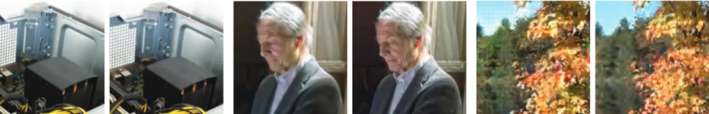
In order to show examples of the artifacts of deep-learning-based methods, we report in Figure 4 some details of coded images. Part (a) of the figure demonstrates a case where Ball´e et al. achieve clearly better visual quality than JPEG 2000 at a higher bitrate. Notice that there are no visible, unnatural ringing or mosquito noise artifacts, nor blocking, and although high-frequency details are somehow blurred, edges
TABLE I
STATISTICAL ANALYSIS OF OBJECTIVE QUALITY METRICS ON THE PROPOSED DATASET(I). BEST METRICS VALUES PER COLUMN ARE HIGHLIGHTED IN BOLD.
JPEG2K BPG Balle Toderici
Metric PCC SROCC RMSE OR PCC SROCC RMSE OR PCC SROCC RMSE OR PCC SROCC RMSE OR
PSNR 0.860 0.873 15.1 0.14 0.851 0.854 16.2 0.20 0.621 0.574 19.7 0.20 0.699 0.707 19.9 0.18 SSIM 0.894 0.892 13.5 0.07 0.915 0.901 12.5 0.07 0.860 0.863 12.8 0.08 0.836 0.824 15.3 0.11 MS-SSIM 0.961 0.958 8.3 0.00 0.971 0.956 7.4 0.00 0.936 0.939 8.9 0.00 0.923 0.898 10.7 0.00 VSNR 0.903 0.907 12.9 0.07 0.889 0.882 14.1 0.10 0.750 0.728 16.6 0.16 0.768 0.738 17.8 0.18 VIF 0.958 0.956 8.7 0.03 0.968 0.949 7.8 0.00 0.929 0.924 9.3 0.04 0.940 0.911 9.5 0.07 UQI 0.833 0.833 16.7 0.23 0.792 0.770 18.9 0.33 0.760 0.752 16.3 0.20 0.863 0.863 14.1 0.04 IFC 0.921 0.915 11.7 0.07 0.931 0.915 11.3 0.07 0.880 0.876 11.9 0.04 0.964 0.932 7.4 0.04 NQM 0.881 0.884 14.3 0.10 0.916 0.905 12.4 0.10 0.793 0.804 15.3 0.12 0.848 0.817 14.7 0.11 WSNR 0.946 0.949 9.8 0.00 0.962 0.953 8.5 0.00 0.896 0.889 11.2 0.04 0.890 0.866 12.7 0.11 TABLE II
STATISTICAL ANALYSIS OF OBJECTIVE QUALITY METRICS ON THE PROPOSED DATASET(II). RESULTS ARE GROUPED CONSIDERING:STANDARD IMAGE CODECS(JPEG 2000ANDBPG);DEEP-LEARNING-BASED COMPRESSION ALGORITHMS;AND ALL THE113STIMULI OF THE DATASET. BEST METRICS
VALUES PER COLUMN ARE HIGHLIGHTED IN BOLD.
JPEG2K & BPG Balle & Toderici All methods
Metric PCC SROCC RMSE PCC SROCC RMSE PCC SROCC RMSE
PSNR 0.858 0.870 15.676 0.652 0.638 20.156 0.763 0.766 18.619 SSIM 0.902 0.908 13.154 0.829 0.830 14.864 0.866 0.871 14.392 MS-SSIM 0.964 0.957 8.170 0.917 0.907 10.6 0.941 0.936 9.77604 VSNR 0.888 0.896 14.011 0.740 0.731 17.881 0.815 0.815 16.677 VIF 0.962 0.953 8.348 0.931 0.919 9.740 0.944 0.936 9.516 UQI 0.812 0.802 17.813 0.815 0.821 15.423 0.813 0.807 16.751 IFC 0.925 0.917 11.615 0.922 0.907 10.282 0.922 0.910 11.163 NQM 0.897 0.899 13.499 0.803 0.794 15.842 0.852 0.848 15.078 WSNR 0.953 0.955 9.261 0.866 0.851 13.318 0.910 0.908 11.914 PSNR 20 30 40 50 MOS 0 20 40 60 80 100 (a) MOS vs PSNR Balle Toderici BPG JPEG2k MS-SSIM 0.7 0.8 0.9 1 MOS 0 20 40 60 80 100 (b) MOS vs MS-SSIM Balle Toderici BPG JPEG2k VIF 0 0.5 1 MOS 0 20 40 60 80 100 (c) MOS vs VIF Balle Toderici BPG JPEG2k
Fig. 3. Scatter plots for MOS against different objective metrics.
and straight lines are generally well preserved. In part (b) of Figure 4, these characteristic artifacts are shown in comparison with a BPG-compressed image at similar bitrate, which has higher MOS. Notice again the sort of “brush” effect for Ball´e, and the little presence of artifacts on high-contrast edges. Finally, in Figure 4(c) we show an example for Toderici against JPEG 2000. The two images have similar bitrates; however, JPEG 2000 has a better PSNR score while Toderici has a higher MOS score. This is interesting to note as the image compressed with Toderici et al. has more details but loses in PSNR most likely due to blocking artifacts. It should be noted that these type of artifacts have been partially suppressed in their follow-up work [23]. However, we did not have access to the updated implementation.
In order to investigate further the distortion of Ball´e and Toderici’s methods, we computed the natural image quality evaluator (NIQE) metric [24] for all stimuli but Screenshot (which is a synthetic image). NIQE measures the distance of the distribution of mean-contrast normalized coefficients of the image under study with respect to a reference distribution
of the same coefficients found on a large dataset of pristine images, and thus is both opinion- and distortion-unaware. Lower values of the metric indicate higher naturalness. Notice that stimuli compressed with both Ball´e and Toderici tend to be more natural, i.e., they follow better the statistics of natural images, than images coded with JPEG 2000.
V. DISCUSSION AND CONCLUSIONS
This is the first, independent study to evaluate subjectively and objectively the quality of two deep-learning-compressed images. On our dataset, both methods achieve results similar to or better than JPEG 2000 in many cases, and in other cases their rate-distortion performance is equivalent to that of BPG. These results are somewhat justified by the more natural appearance of images compressed by the two deep-learning-based methods, compared, e.g., to JPEG 2000. The reason for this is most probably related to the much more powerful generative model expressed by deep auto-encoders, compared to simple image transforms such as DCT and wavelets (in the case of BPG, the use of in-loop filters considerably reduces
(a) (left) Ball´e, 0.38 bpp; (right) JPEG 2K, 0.43 bpp (b) (left) Ball´e, 0.09 bpp; (right) BPG, 0.08 bpp (c)(left)Toderici,0.125 bpp; (right)JPEG 2K, 0.1 bpp Fig. 4. Examples of images (details) coded with different methods. (a) A case where an image coded with the method of Ball´e et al. has better quality than JPEG 2000 at a similar bitrate. (b) An example where Ball´e et al. has worse quality than BPG. (c) An example of Toderici et al. has better quality in MOS (12.4 vs 8.1) but lower in PSNR (20.85dBs vs 21.35dBs). bitrate (bpp) 0 0.5 1 NIQE 0 5 10 15 NIQE vs Bitrate Balle Toderici BPG JPEG2k Original
Fig. 5. Natural Image Quality Evaluator (NIQE) metric, compute for different compression methods. Only bitrates below 1.2 bpp are reported. Black squares indicate the values of NIQE for the pristine contents.
the visibility of blocking, at the advantage of naturalness). A direct consequence is that simple pixel-based metrics such as the PSNR, which are still widely used in image and video coding, are much less accurate to judge visual quality with the new methods.
A more detailed analysis would require coding images at the same (or as close as possible) bitrate and conduct pairwise comparison tests to evaluate precisely the preferences of observers. However, this is difficult at this stage as the available implementations of Ball´e et al. [14] and Toderici et al. [15] do not enable a fine-granularity rate control. Yet, our results are still surprising, when thinking that BPG and JPEG 2000 are the product of decades of coding optimization and engineering, while the methods of Ball´e et al. [14] and Toderici et al. [15] are proofs of concept developed in the last year. This suggests a great potential in using deep generative models for next-generation image and video codecs.
REFERENCES
[1] A. Gersho and R. M. Gray, Vector Quantization and Signal Compression. Springer Science & Business Media, 1991, vol. 159.
[2] N. Ahmed, T. Natarajan, and K. R. Rao, “Discrete cosine transform,”
IEEE transactions on Computers, vol. 100, no. 1, pp. 90–93, 1974.
[3] S. Mallat, A wavelet tour of signal processing. Academic press, 1999. [4] I. Tosic and P. Frossard, “Dictionary learning,” IEEE Signal Processing
Magazine, vol. 28, no. 2, pp. 27–38, March 2011.
[5] L. Theis, W. Shi, A. Cunningham, and F. Husz´ar, “Lossy image compression with compressive autoencoders,” in Int. Conf. on Learning
Representations (ICLR), Toulon, France, Apr. 2017.
[6] E. Agustsson, F. Mentzer, M. Tschannen, L. Cavigelli, R. Timofte, L. Benini, and L. V. Gool, “Soft-to-hard vector quantization for end-to-end learning compressible representations,” in Advances in Neural
Information Processing Systems, 2017, pp. 1141–1151.
[7] D. Minnen, G. Toderici, M. Covell, T. Chinen, N. Johnston, J. Shor, S. J. Hwang, D. Vincent, and S. Singh, “Spatially adaptive image compression using a tiled deep network,” in 2017 IEEE International Conference on
Image Processing (ICIP), Sept 2017, pp. 2796–2800.
[8] O. Rippel and L. Bourdev, “Real-time adaptive image compression,”
arXiv preprint arXiv:1705.05823, 2017.
[9] J. Ball´e, D. Minnen, S. Singh, S. J. Hwang, and N. Johnston, “Variational image compression with a scale hyperprior,” in Int. Conf. on Learning
Representations (ICLR), Vancouver, CA, May 2018.
[10] E. Agustsson, M. Tschannen, F. Mentzer, R. Timofte, and L. Van Gool, “Generative adversarial networks for extreme learned image compres-sion,” arXiv preprint arXiv:1804.02958, 2018.
[11] D. P. Kingma and M. Welling, “Auto-encoding variational bayes,” in
Int. Conf. on Learning Representations (ICLR), Banff, CA, Apr. 2014.
[12] I. Goodfellow, A. Courville, and Y. Bengio, Deep learning. MIT press Cambridge, 2016, vol. 1.
[13] S. Santurkar, D. Budden, and N. Shavit, “Generative compression,” arXiv
preprint arXiv:1703.01467, 2017.
[14] J. Ball´e, V. Laparra, and E. P. Simoncelli, “End-to-end optimized image compression,” in Int. Conf. on Learning Representations (ICLR), Toulon, France, Apr. 2017.
[15] G. Toderici, D. Vincent, N. Johnston, S. J. Hwang, D. Minnen, J. Shor, and M. Covell, “Full resolution image compression with recurrent neural networks,” in IEEE Int. Conf. on Computer Vision and Pattern
Recognition (CVPR), Honolulu, Hawaii, USA, Jul. 2017, pp. 5435–5443.
[16] J. Froehlich, S. Grandinetti, B. Eberhardt, S. Walter, A. Schilling, and H. Brendel, “Creating cinematic wide gamut HDR-video for the evaluation of tone mapping operators and HDR-displays,” in Digital
Photography X, vol. 9023. International Society for Optics and Photonics, 2014, p. 90230X.
[17] M. D. Fairchild, “The HDR photographic survey,” in Color and Imaging
Conference, vol. 2007, no. 1. Society for Imaging Science and Technology, 2007, pp. 233–238.
[18] R. Mantiuk, S. Daly, and L. Kerofsky, “Display adaptive tone mapping,” in ACM Transactions on Graphics (TOG), vol. 27, no. 3. ACM, 2008, p. 68.
[19] V. Hulusic, K. Debattista, G. Valenzise, and F. Dufaux, “A model of perceived dynamic range for HDR images,” Signal Processing: Image
Communication, vol. 51, pp. 26–39, 2017.
[20] ITU-R, “Methodology for the subjective assessment of the quality of television pictures,” ITU-R Recommendation BT.500-13, 2012. [21] ITU-T, “Methods, metrics and procedures for statistical evaluation,
qualification and comparison of objective quality prediction models,”
ITU-T Recommendation P.1401, 2012.
[22] H. R. Sheikh, M. F. Sabir, and A. C. Bovik, “A statistical evaluation of recent full reference image quality assessment algorithms,” IEEE
Transactions on image processing, vol. 15, no. 11, pp. 3440–3451, 2006.
[23] N. Johnston, D. Vincent, D. Minnen, M. Covell, S. Singh, T. Chinen, and S. J. Hwang, “Improved lossy image compression with priming and spatially adaptive bit rates for recurrent networks,” arXiv:1703.10114v1, 2017.
[24] A. Mittal, R. Soundararajan, and A. C. Bovik, “Making a “completely blind” image quality analyzer,” IEEE Signal Processing Letters, vol. 20, no. 3, pp. 209–212, 2013.