Universit´e de Montr´eal
Deep learning of representations and its application to computer vision
par Ian Goodfellow
D´epartement d’informatique et de recherche op´erationnelle Facult´e des arts et des sciences
Th`ese pr´esent´ee `a la Facult´e des arts et des sciences en vue de l’obtention du grade de Philosophiæ Doctor (Ph.D.)
en informatique
Résumé
L’objectif de cette th`ese par articles est de pr´esenter modestement quelques ´etapes du parcours qui m`enera (on esp`ere) `a une solution g´en´erale du probl`eme de l’intelligence artificielle. Cette th`ese contient quatre articles qui pr´esentent chacun une di↵´erente nouvelle m´ethode d’inf´erence perceptive en utilisant l’apprentissage machine et, plus particuli`erement, les r´eseaux neuronaux profonds. Chacun de ces documents met en ´evidence l’utilit´e de sa m´ethode propos´ee dans le cadre d’une tˆache de vision par ordinateur. Ces m´ethodes sont applicables dans un contexte plus g´en´eral, et dans certains cas elles ont ´et´e appliqu´ees ailleurs, mais ceci ne sera pas abord´e dans le contexte de cette de th`ese.
Dans le premier article, nous pr´esentons deux nouveaux algorithmes d’inf´erence variationelle pour le mod`ele g´en´eratif d’images appel´e codage parcimonieux “spike-and-slab” (CPSS). Ces m´ethodes d’inf´erence plus rapides nous permettent d’utiliser des mod`eles CPSS de tailles beaucoup plus grandes qu’auparavant. Nous d´emon-trons qu’elles sont meilleures pour extraire des d´etecteur de caract´eristiques quand tr`es peu d’exemples ´etiquet´es sont disponibles pour l’entraˆınement. Partant d’un mod`ele CPSS, nous construisons ensuite une architecture profonde, la machine de Boltzmann profonde partiellement dirig´ee (MBP-PD). Ce mod`ele a ´et´e con¸cu de mani`ere `a simplifier d’entraˆınement des machines de Boltzmann profondes qui n´e-cessitent normalement une phase de pr´e-entraˆınement glouton pour chaque couche. Ce probl`eme est r´egl´e dans une certaine mesure, mais le coˆut d’inf´erence dans le nouveau mod`ele est relativement trop ´elev´e pour permettre de l’utiliser de mani`ere pratique.
Dans le deuxi`eme article, nous revenons au probl`eme d’entraˆınement joint de machines de Boltzmann profondes. Cette fois, au lieu de changer de famille de mod`eles, nous introduisons un nouveau crit`ere d’entraˆınement qui donne naissance aux machines de Boltzmann profondes `a multiples pr´edictions (MBP-MP). Les MBP-MP sont entraˆınables en une seule ´etape et ont un meilleur taux de succ`es en classification que les MBP classiques. Elles s’entraˆınent aussi avec des m´ethodes variationelles standard au lieu de n´ecessiter un classificateur discriminant pour ob-tenir un bon taux de succ`es en classification. Par contre, un des inconv´enients de tels mod`eles est leur incapacit´e de g´en´erer des ´echantillons, mais ceci n’est pas trop grave puisque la performance de classification des machines de Boltzmann pro-fondes n’est plus une priorit´e ´etant donn´e les derni`eres avanc´ees en apprentissage supervis´e. Malgr´e cela, les MBP-MP demeurent int´eressantes parce qu’elles sont ca-pable d’accomplir certaines tˆaches que des mod`eles purement supervis´es ne peuvent
Le travail pr´esent´e dans cette th`ese s’est d´eroul´e au milieu d’une p´eriode de transformations importantes du domaine de l’apprentissage `a r´eseaux neuronaux profonds qui a ´et´e d´eclench´ee par la d´ecouverte de l’algorithme de “dropout” par Geo↵rey Hinton. Dropout rend possible un entraˆınement purement supervis´e d’ar-chitectures de propagation unidirectionnel sans ˆetre expos´e au danger de sur-entraˆınement. Le troisi`eme article pr´esent´e dans cette th`ese introduit une nouvelle fonction d’activation sp´ecialement con¸cue pour aller avec l’algorithme de Dropout. Cette fonction d’activation, appel´ee maxout, permet l’utilisation de aggr´egation multi-canal dans un contexte d’apprentissage purement supervis´e. Nous d´emon-trons comment plusieurs tˆaches de reconnaissance d’objets sont mieux accomplies par l’utilisation de maxout.
Pour terminer, sont pr´esentons un vrai cas d’utilisation dans l’industrie pour la transcription d’adresses de maisons `a plusieurs chi↵res. En combinant maxout avec une nouvelle sorte de couche de sortie pour des r´eseaux neuronaux de convolution, nous d´emontrons qu’il est possible d’atteindre un taux de succ`es comparable `a celui des humains sur un ensemble de donn´ees coriace constitu´e de photos prises par les voitures de Google. Ce syst`eme a ´et´e d´eploy´e avec succ`es chez Google pour lire environ cent million d’adresses de maisons.
Mots-cl´es: r´eseau de neurones, apprentissage profond, apprentissage non su-pervis´e, apprentissage susu-pervis´e, apprentissage semi-susu-pervis´e, machines de Boltz-mann, les mod`eles bas´es sur l’´energie, l’inference variationnel, l’apprentissage va-riationnel, le codage parcimonieux, r´eseaux neuronaux de convolution, la fonction d’activation, “dropout,” la reconnaissance d’objets, transcription, reconnaissance optique de caract`eres, g´eocodage, entr´ees manquantes
Summary
The goal of this thesis is to present a few small steps along the road to solving general artificial intelligence. This is a thesis by articles containing four articles. Each of these articles presents a new method for performing perceptual inference using machine learning and deep architectures. Each of these papers demonstrates the utility of the proposed method in the context of a computer vision task. The methods are more generally applicable and in some cases have been applied to other kinds of tasks, but this thesis does not explore such applications.
In the first article, we present two fast new variational inference algorithms for a generative model of images known as spike-and-slab sparse coding (S3C). These faster inference algorithms allow us to scale spike-and-slab sparse coding to unprecedented problem sizes and show that it is a superior feature extractor for object recognition tasks when very few labeled examples are available. We then build a new deep architecture, the partially-directed deep Boltzmann machine (PD-DBM) on top of the S3C model. This model was designed to simplify the training procedure for deep Boltzmann machines, which previously required a greedy layer-wise pretraining procedure. This model partially succeeds at solving this problem, but the cost of inference in the new model is high enough that it makes scaling the model to serious applications difficult.
In the second article, we revisit the problem of jointly training deep Boltz-mann machines. This time, rather than changing the model family, we present a new training criterion, resulting in multi-prediction deep Boltzmann machines (MP-DBMs). MP-DBMs may be trained in a single stage and obtain better classification accuracy than traditional DBMs. They also are able to classify well using standard variational inference techniques, rather than requiring a separate, specialized, dis-criminatively trained classifier to obtain good classification performance. However, this comes at the cost of the model not being able to generate good samples. The classification performance of deep Boltzmann machines is no longer especially inter-esting following recent advances in supervised learning, but the MP-DBM remains interesting because it can perform tasks that purely supervised models cannot, such as classification in the presence of missing inputs and imputation of missing inputs. The general zeitgeist of deep learning research changed dramatically during the midst of the work on this thesis with the introduction of Geo↵rey Hinton’s dropout algorithm. Dropout permits purely supervised training of feedforward architectures with little overfitting. The third paper in this thesis presents a new activation function for feedforward neural networks which was explicitly designed to work
supervised manner. We demonstrate improvements on several object recognition tasks using this activation function.
Finally, we solve a real world task: transcription of photos of multi-digit house numbers for geo-coding. Using maxout units and a new kind of output layer for convolutional neural networks, we demonstrate human level accuracy (with limited coverage) on a challenging real-world dataset. This system has been deployed at Google and successfully used to transcribe nearly 100 million house numbers. Keywords: neural network, deep learning, unsupervised learning, supervised learning, semi-supervised learning, Boltzmann machines, energy-based models, vari-ational inference, varivari-ational learning, feature learning, sparse coding, convolutional networks, activation function, dropout, pooling, object recognition, transcription, optical character recognition, inpainting, missing inputs
Contents
R´esum´e . . . ii
Summary . . . iv
Contents . . . vi
List of Figures. . . x
List of Tables . . . xii
1 Machine Learning . . . 1
1.1 Introduction to Machine Learning . . . 1
1.1.1 Generalization and the IID assumptions . . . 3
1.1.2 Maximum likelihood estimation . . . 4
1.1.3 Optimization . . . 5
1.2 Supervised learning . . . 8
1.2.1 Support vector machines and statistical learning theory . . . 9
1.3 Unsupervised learning . . . 11
1.4 Feature learning . . . 12
2 Structured Probabilistic Models . . . 17
2.1 Directed models . . . 17
2.2 Undirected models . . . 18
2.2.1 Sampling . . . 20
2.3 Latent variables . . . 21
2.3.1 Latent variables versus structure learning . . . 21
2.3.2 Latent variables for feature learning . . . 22
2.4 Stochastic approximations to maximum likelihood . . . 23
2.4.1 Example: The restricted Boltzmann machine . . . 25
2.5 Variational approximations. . . 26
2.5.1 Variational learning . . . 27
2.6 Combining approximations: The deep Boltzmann machine . . . 29
3 Supervised deep learning . . . 31
4 Prologue to First Article . . . 36
4.1 Article Details . . . 36
4.2 Context . . . 36
4.3 Contributions . . . 37
4.4 Recent Developments . . . 38
5 Scaling up Spike-and-Slab Models for Unsupervised Feature Learn-ing . . . 39
5.1 Introduction . . . 39
5.2 Models . . . 42
5.2.1 The spike-and-slab sparse coding model. . . 42
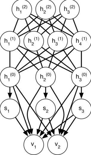
5.2.2 The partially directed deep Boltzmann machine model . . . 42
5.3 Learning procedures . . . 45
5.3.1 Avoiding greedy pretraining . . . 46
5.4 Inference procedures . . . 47
5.4.1 Variational inference for S3C. . . 48
5.4.2 Variational inference for the PD-DBM . . . 51
5.5 Comparison to other feature encoding methods . . . 52
5.5.1 Comparison to sparse coding. . . 52
5.5.2 Comparison to restricted Boltzmann machines . . . 53
5.5.3 Other related work . . . 56
5.6 Runtime results . . . 56
5.7 Classification results . . . 59
5.7.1 CIFAR-10 . . . 61
5.7.2 CIFAR-100 . . . 62
5.7.3 Transfer learning challenge . . . 62
5.7.4 Ablative analysis . . . 63
5.8 Sampling results. . . 64
5.9 Conclusion . . . 67
6 Prologue to Second Article . . . 69
6.1 Article Details . . . 69
6.2 Context . . . 69
6.3 Contributions . . . 70
6.4 Recent Developments . . . 70
7.3 Motivation . . . 73
7.4 Methods . . . 74
7.4.1 Multi-prediction Training . . . 74
7.4.2 The Multi-Inference Trick . . . 76
7.4.3 Justification and advantages . . . 82
7.4.4 Regularization . . . 83
7.4.5 Related work: centering . . . 84
7.4.6 Sampling, and a connection to GSNs . . . 84
7.5 Experiments . . . 85
7.5.1 MNIST experiments . . . 85
7.5.2 NORB experiments . . . 86
7.6 Conclusion . . . 87
8 Prologue to Third Article . . . 89
8.1 Article Details . . . 89 8.2 Context . . . 89 8.3 Contributions . . . 90 8.4 Recent Developments . . . 90 9 Maxout Networks . . . 91 9.1 Introduction . . . 91 9.2 Review of dropout . . . 92 9.3 Description of maxout . . . 93
9.4 Maxout is a universal approximator . . . 95
9.5 Benchmark results . . . 96
9.5.1 MNIST . . . 97
9.5.2 CIFAR-10 . . . 98
9.5.3 CIFAR-100 . . . 99
9.5.4 Street View House Numbers . . . 100
9.6 Comparison to rectifiers . . . 101
9.7 Model averaging. . . 102
9.8 Optimization . . . 103
9.8.1 Optimization experiments . . . 104
9.8.2 Saturation . . . 104
9.8.3 Lower layer gradients and bagging . . . 105
9.9 Conclusion . . . 105
10 Prologue to Fourth Article . . . 112
10.1 Article Details . . . 112
10.4 Recent Developments . . . 113
11 Multi-digit Number Recognition from Street View Imagery us-ing Deep Convolutional Neural Networks . . . 114
11.1 Introduction . . . 114
11.2 Related work . . . 115
11.3 Problem description. . . 117
11.4 Methods . . . 119
11.5 Experiments . . . 120
11.5.1 Public Street View House Numbers dataset. . . 120
11.5.2 Internal Street View data . . . 121
11.5.3 Performance analysis . . . 124
11.5.4 Application to Geocoding . . . 125
11.6 Discussion . . . 126
12 General conclusion . . . 129
A Example transcription network inference . . . 131
List of Figures
1.1 Feature learning example . . . 13
1.2 Deep learning example . . . 15
2.1 An example RBM drawn as a Markov network . . . 25
2.2 An example graph of a deep Boltzmann machine. . . 30
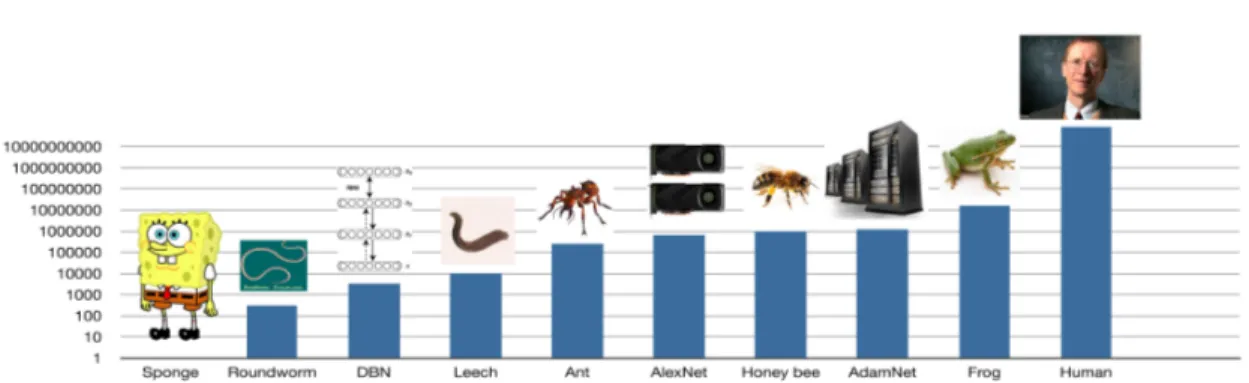
3.1 Number of neurons in animals and machine learning models . . . . 34
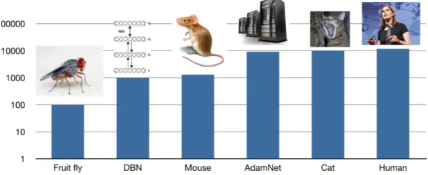
3.2 Average number of connections per neuron in animals and machine learning models . . . 35
5.1 A graphical model depicting an example PD-DBM. . . 44
5.2 Histogram of feature values . . . 47
5.3 Iterative sparsification of S3C features . . . 48
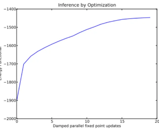
5.4 Inference by minimizing variational free energy. . . 51
5.5 Scale of S3C problems . . . 58
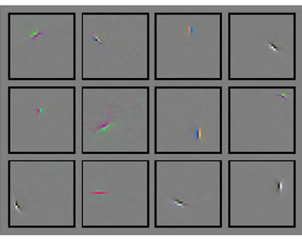
5.6 Example S3C filters . . . 58
5.7 Inference speed . . . 59
5.8 Classification with limited amounts of labeled examples . . . 60
5.9 CIFAR-100 classification . . . 60
5.10 Performance of several limited variants of S3C . . . 63
5.11 S3C samples . . . 64
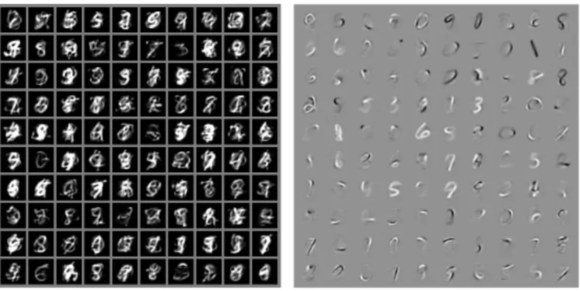
5.12 DBM and PD-DBM samples . . . 65
5.13 DBM and PD-DBM weights . . . 66
7.1 Greedy layerwise training of a DBM. . . 76
7.2 Multi-prediction training . . . 77
7.3 Mean field inference applied to MNIST digits . . . 78
7.4 Multi-inference trick . . . 79
7.5 GSN-style samples from an MP-DBM . . . 80
7.6 Quantitive results on MNIST . . . 85
9.1 Using maxout to implement pre-existing activation functions . . . . 94
9.2 The activations of maxout units are not sparse. . . 94
9.6 Comparison to rectifier networks. . . 107
9.7 Monte Carlo classification . . . 108
9.8 KL divergence from Monte Carlo predictions . . . 109
9.9 Optimization of deep models . . . 110
9.10 Avoidance of “dead units” . . . 111
11.1 Example input image and graph of transcriber output . . . 117
11.2 Correctly classified difficult examples . . . 122
11.3 Incorrectly classified examples . . . 123
11.4 Classification accuracy improves with depth . . . 125
11.5 Geocoding example . . . 128
List of Tables
9.1 Permutation invariant MNIST classification . . . 97
9.2 Convolutional MNIST classification . . . 98
9.3 CIFAR-10 classification . . . 99
9.4 CIFAR-100 classification . . . 101
List of Abbreviations
AIS Annealed Importance Sampling CD Contrastive Divergence
CNN Convolutional Neural Network DBM Deep Boltzmann Machine
DBN Deep Belief Network EBM Energy-Based Model
EM Expectation Maximization
(GP)-GPU (General Purpose) Graphics Processing Unit GSN Generative Stochastic Network
I.I.D Independent and Identically-Distributed KL Kullback-Leibler
LBFGS Limited-memory Boyden-Fletcher-Goldfarb-Shanno algorithm MAP Maximum a posteriori
mcRBM Mean-Covariance Restricted Boltzmann Machine MLP Multi-Layer Perceptron
MP-DBM Multi-Prediction Deep Boltzmann Machine MPT Multi-Prediction Training
NADE Neural Autoregressive Distribution Estimator NN Neural Network
OCR Optical Character Recognition OMP Orthogonal Matching Pursuit
PCD Persistent Contrastive Divergence (also SML) PD-DBM Partially Directed Deep Boltzmann Machine
PDF Probability Density Function PWL Piece-Wise Linear
RBF Radial Basis Function
RBM Restricted Boltzmann Machine SRBM Semi-Restricted Boltzmann Machine
S3C Spike-and-Slab Sparse Coding SC Sparse Coding
SGD Stochastic Gradient Descent
SML Stochastic Maximum Likelihood (also PCD) ssRBM Spike & Slab Restricted Boltzmann Machine
SVHN Street View House Numbers SVM Support Vector Machine
Acknowledgments
I’d like to thank many people who helped me along my path to writing this thesis.
I’d especially like to thank my thesis advisor, Yoshua Bengio, for taking me under his wing, and for running a lab where so many researchers are so free to explore creative ideas. I’d also like to thank my co-advisor Aaron Courville, for all of his advice and knowledge he has shared with me.
All of my co-authors–Aaron Courville, Yoshua Bengio, David Warde-Farley, Mehdi Mirza, Yaroslav Bulatov, Julian Ibarz, Sacha Arnoud, and Vinay Shet–were a pleasure to work with, and I could not have written this thesis without them.
I’d like to thank several people at Stanford who were instrumental in getting me interested in machine learning and starting me along this path, including Jerry Cain, Andrew Ng, Daphne Koller, Ethan Dreyfuss, Stephen Gould, and Andrew Saxe.
I’d like to thank Google for awarding me the Google PhD Fellowship in Deep Learning. The fellowship has given me the freedom to spend time on projects like the Pylearn2 open source machine learning library and helping Yoshua write a textbook on deep learning.
I’d like to thank Fr´ed´eric Bastien for keeping all of the computing and software infrastructure at LISA running smoothly, and helping get convolutional networks running fast in Theano.
I’d like to thank Guillaume Alain and Nicolas Boulanger-Lewandowski for their help translating the summary of this thesis into French. I’d like to thank Guillaume Alain, Kyungyun Cho, and Paula Goodfellow for their feedback on drafts of this thesis. I’d like to thank David Warde-Farley and Nicolas Boulanger-Lewandowski for help with various LATEX commands, and Guillaume Desjardins for letting me
copy the basic LATEX template for a Universit´e de Montr´eal PhD thesis from his
own.
Several members of the LISA lab made LISA a fun and intellectual atmosphere. I’d especially like to thank David Warde-Farley, Yann Dauphin, Mehdi Mirza, Li Yao, Guillaume Desjardins, James Bergstra, Razvan Pascanu, and Guillaume Alain for many good lunches, fun game nights, and interesting discussions.
I’d like to thank the people I worked with at Google for making my internship an enjoyable time and providing a lot of help and mentorship. In addition to my co-authors mentioned above, I’d especially like to thank Samy Bengio, Rajat Monga, Marc’Aurelio Ranzato, and Ilya Sutskever.
I’d like to thank my parents, Val and Paula Goodfellow, for raising me to value education education. My grandmother Jalaine was especially adamant that I pursuse a PhD.
I first arrived in Montr´eal. I’d like to thank David Warde-Farley for helping me throw my couch o↵ my fourth story balcony. I’d like to thank my friend Sarah for her seemingly infinite patience and support; without her it’s hard to imagine how I would have survived the foreign student experience. I’d like to thank my friend and exercise partner Claire for helping me stay in shape while working hard on my research. Finally, I’d like to thank my girlfriend Daniela for all of her support and understanding, and the many sacrifices she’s made to let me continue pursuing my research.
1
Machine Learning
This thesis focuses on advancing the state of the art of machine perception, with a particular focus on computer vision. Computer vision and many other forms of machine perception are too difficult to solve by manually designing rules for processing inputs. Instead, some degree of learning is necessary. My personal view is that nearly the entire perception system should be learned.
Throughout the rest of this thesis, the narrator will be referred to as “we,” rather than “I.” This is because, as a thesis by articles, this thesis presents research conducted in a collaborative setting. It should be understood that the writing outside of the articles themselves is my own.
This chapter provides some background on machine learning in general. The subsequent chapters give more background on the particular kinds of machine learn-ing used in the rest of the thesis. The remainder of the thesis presents the articles containing new methods.
1.1
Introduction to Machine Learning
Machine learning is the study of designing machines (or more commonly, soft-ware for general purpose machines) that can learn from data. This is useful for solving a variety of tasks, including computer vision, for which the solution is too difficult for a human software engineer to specify in terms of a fixed piece of soft-ware. Moreover, since learning is a critical part of intelligence, studying machine learning can shed light on the principles that govern intelligence.
But what exactly does it mean for a machine to learn? A commonly-cited definition is “A computer program is said to learn from experience E with respect to some class of tasks T and performance measure P , if its performance at tasks
imagine a very wide variety of experiences E, tasks T , and performance measures P .
In this work, the experience E always includes the experience of observing a set of examples encoded in a design matrix X 2 Rm⇥n. Each of the m rows of
X represents a di↵erent example which is described by n features. For computer vision tasks in which the examples are images, each feature is the intensity of a di↵erent pixel in the image.
For most but not all of the experiments in this thesis, the experience E also includes observing a label for each of the examples. For classification tasks such as object recognition, the labels are encoded in a vector y2 {1, . . . , k}m, with element
yi specifying which of k object classes example i belongs to. Each numeric value
in the domain of yi corresponds to a real-world category, e.g. 0 can mean “dogs”, 1
can mean “cats”, 2 can mean “cars”, etc.
In some experiments in this thesis, the label for each example is a vector, speci-fying a sequence of symbols to associate with each example. This is used in chapter 11for transcribing multi-digit house numbers from photos.
Machine learning researchers study very many di↵erent tasks T . In this work, we explore the following tasks:
— Density estimation: In this task, the machine learning algorithm is asked to learn a function pmodel : Rn ! R, where pmodel(x) can be interpreted as
a probability density function on the space that the examples were drawn from. To do this task well (we’ll specify exactly what that means when we discuss performance measures P ), the algorithm needs to learn the structure of the data it has seen. It must know where examples cluster tightly and where they are unlikely to occur.
— Imputation of missing values: In this task, the machine learning algorithm is given a new example x2 Rn, but with some entries x
i of x missing. The
algorithm must provide a prediction of the values of the missing entries. This task is closely related to density estimation, because it can be solved by learning pmodel(x) then conditioning on the observed entries of x.
— Classification: In this task, the algorithm is asked to output a function f : Rn ! {1, . . . , k}. Here f(x) can be interpreted as an estimate of the
thesis does not make any extensive use of the probability distribution over classes.
— Classification with missing inputs : This is similar to classification, except rather than providing a single classification function, the algorithm must learn a set of functions. Each function corresponds to classifying x with a di↵erent subset of its inputs missing.
— Transcription : This is similar to classification, except that the output is a sequence of symbols, rather than a single symbol.
Each of these tasks must be evaluated with a performance measure P . For the density estimation task, one could define a new set of examples X(test) and measure
the probability of these examples according to the model. Evaluating the perfor-mance of a density estimation algorithm is difficult and we often turn to proxies for this value. For missing values imputation, we can measure the conditional proba-bility the model assigns to the missing pixels in the test set, or some proxy thereof. For the classification and related tasks, one could define a set of labels y(test), and
measure the classification accuracy of the model, i.e., the frequency with which f (X(test)i,: ) = y(test)i .
1.1.1
Generalization and the IID assumptions
An important aspect of the performance measures described above is that they both depend on a test set of data not seen during the learning process. This means that the learning algorithm must be able to generalize to new examples. Generalization is what makes machine learning di↵erent from optimization.
In order to be able to generalize from the training set to the test set, one needs to assume that there is some common structure in the data. The most commonly used set of assumptions are the i.i.d. assumptions . These assumptions state that the data is independently and identically distributed: each example is generated independently from the other examples, and each example is drawn from the same distribution pdata (Cover, 2006) . Formally,
pdata(X, y) = ⇧ipdata(Xi:, yi).
de-1.1.2
Maximum likelihood estimation
An extremely popular approach to machine learning is maximum likelihood es-timation. In this approach, one defines a probabilistic model that is controlled by a set of parameters ✓. The model provides a probability distribution pmodel(x; ✓) over
examples x. (In this work we do not explore non-parametric modeling in which p is some function of the training set which can not be encoded in a fixed-length parameter vector) One can then use a statistical estimator to obtain the correct value of ✓, drawn from set ⇥ of permissible values.
The estimator used in maximum likelihood is
ˆ
✓ = argmax✓2⇥⇧ipmodel(Xi:; ✓)
= argmax✓2⇥X
i
log pmodel(Xi:; ✓).
In other words, the maximum likelihood estimation procedure is to pick the parameters that maximize the probability that the model will generate the training data. As shown above, one usually exploits the monotonically increasing property of the logarithm and instead optimizes the log likelihood, an alternative criterion which is maximized by the same value of ✓. The log likelihood is more convenient to work with than the likelihood. As a product of several factors in the interval [0, 1], computing the likelihood on a digital computer often results in numerical underflow. The log likelihood avoids this difficulty. It also conveniently decomposes into a sum over separate examples, which makes many forms of mathematical analysis more convenient.
To justify the maximum likelihood estimation approach, assume that pdata(x)2
{pmodel(x; ✓), ✓ 2 ⇥}. Given this and the i.i.d assumptions one can prove that in
the limit of infinite data, the maximum likelihood estimator recovers a pmodel that
matches pdata. Note that we claim we can recover the true probability distribution,
not the true value of ✓. This is because the value of ✓ that was used to generate the training data cannot be determined if multiple values of ✓ correspond to the same probability distribution. The ability of the estimator to asymptotically recover the correct distribution is called consistency (Newey and McFadden, 1994).
well without infinite data. In the case of finite data, the maximum likelihood es-timator is not always the best possible approach. In cases where very little data is available, maximum likelihood estimation of parametric models performs poorly compared to other approaches such as Bayesian inference (in which one makes new predictions by integrating over all possible values of ✓). Unfortunately, the family of models for which this integral can be evaluated analytically is extremely limited. Bayesian inference usually entails computationally expensive Monte Carlo approximations. In practice, a commonly used middle ground between maximum likelihood and Bayesian inference is to use an estimator which has been regular-ized. This usually has roughly the same computation cost as maximum likelihood yet generalizes better. Regularization is often achieved by biasing the maximum likelihood estimator so that new predictions from the model will resemble those obtained by Bayesian inference. Typically this means maximizing a function with two terms, one term being the log likelihood of the data given ✓ and the other being the log likelihood of ✓ under some prior. This is equivalent to performing Bayesian inference by approximating the integral over all ✓ with a Dirac distribution centered on the MAP estimate of ✓.
In this work, we usually use maximum likelihood estimation only in situations where at least tens of thousands of examples are available, and we typically use at least one form of regularization. With this amount of data available, it is reasonable to expect maximum likelihood to do a good job of recovering ✓, especially when using regularization.
1.1.3
Optimization
Much of machine learning can be cast as optimization. In the case of maxi-mum likelihood estimation, one can define an objective function given by the log likelihood
`(✓) = X
i
log pmodel(Xi:; ✓)
and solve the optimization problem
maximize `(✓) subject to ✓2 ⇥.
Sometimes this can be done simply by analytically solving r✓`(✓) = 0 for ✓.
Other times, there is no closed-form solution to that equation and the solution must be obtained by an iterative optimization method.
One of the simplest iterative optimization methods is gradient ascent. This algorithm is based on the observation that r✓`(✓) gives the direction in which `
increases most rapidly in a local neighborhood around ✓. The idea is to take small steps in the direction of the gradient.
On iteration t of the gradient ascent algorithm, we compute the updated value of ✓ using the following rule:
✓(t) = ✓(t 1)+ ↵(t)r✓`(✓)
where ↵(t) is a positive scalar controlling the size of the step (Bishop, 2006, Chapter 3) . The scalar ↵ is commonly referred to as the learning rate.
Gradient ascent may be expensive if there is a lot of redundancy in the dataset. It may take only a small number of examples to get a good estimate of the direction of the gradient from the current value of ✓ but gradient ascent will compute the gradient contribution of every single example in the dataset. As an extreme case, consider the behavior of gradient ascent when all m examples in the training set are the same as each other. In this case, the cost of computing the gradient is m times what is necessary to obtain the correct step direction. More generally, consider the standard error of the mean of our estimate of the gradient. The denominator is p
m, meaning that the error of our estimate of the true gradient decreases slower than linearly as we add more examples. Because the computation of the estimate increases linearly, it is usually not computationally cost-e↵ective to use a large number of examples to estimate the gradient.
An alternative algorithm resolves this problem. In stochastic gradient ascent (Bishop, 2006, Chapter 3) , use the following update rule:
✓(t) = ✓(t 1)+ ↵(t)r✓
X
i2S
log pmodel(Xi:; ✓)
where S is a random subset of {1, . . . , m}. The randomly selected training examples are called a minibatch. Typical minibatch sizes range from 1 to 128.
characterized, and we do not explore them here.
When training deep neural nets, it is important to enhance stochastic gradient ascent with a technique called momentum. Momentum is a computationally inex-pensive modification of stochastic gradient ascent where the parameters move with a velocity that is influenced by the gradient at each step:
v(t) = µ(t)v(t 1)+ ↵(t)r✓
X
i2S
log pmodel(Xi:; ✓)
✓(t) = ✓(t 1)+ v(t)
While standard gradient ascent follows the steepest direction at each step, mo-mentum partially accounts for the curvature of the function. Sutskever et al.(2013) showed that this simple method can perform as well as much more complicated second order methods like Hessian-free optimization (Nocedal and Wright, 2006; Martens, 2010).
In this introduction we have presented the optimization in terms of ascending the log likelihood, but in practice the optimization technique is most broadly known as stochastic gradient descent (SGD). In this case, the learning rule is presented as descending a cost function. One can of course ascend the log likelihood by descending the negative log likelihood.
A machine learning practictioner has two main ways of influencing the results of training a model with a gradient method.
One is picking the function ↵(t) that determines how the learning rate evolves over time (and the µ(t) function when using momentum). Constant ↵ often works well, as does a linearly decreasing ↵(t). For µ(t), it is often e↵ective to begin at 0.5 and linearly increase to a value around 0.9.
The other parameter under the practitioner’s control is the convergence crite-rion. A common practice is to halt if `(✓) (evaluated on a held-out validation set) does not increase very much after some number of passes through the dataset. In some cases it is infeasible to compute `(✓) but learning is possible so long as one can computer✓`(✓) or a reasonable approximation thereof. In these cases we must
design other proxies to use to determine convergence.
the model memorizes spurious patterns in the training set and as a result obtains much worse accuracy on the test set. Generally, in machine learning applications, we care about performance on the test set, which we can estimate by monitoring performance on a held out validation set. The best criteria for deep learning usually are based on validation set performance. The main goal of such criteria is to prevent overfitting, not to make sure that a maximum has been reached. A common approach is to store the parameters that have attained the best accuracy on the validation set, and stop training when no new best parameters have been found within some fixed number of update steps. At the end of training, we use the best stored parameters, not the last parameters visited by SGD.
Many other sophisticated optimization algorithms exist, but they have not proven as e↵ective for deep learning as stochastic gradient and momentum have.
1.2
Supervised learning
Supervised learning is the class of learning problems where the desired output of the model on some training set is known in advance and supplied by a supervisor. One example of this is the aforementioned classification problem, where the learned model is a function f (x) that maps examples x to category IDs. Another common supervised learning problem is regression. In the context of regression, the training set consists of a design matrix X and a vector of real-valued targets y2 Rm (or a
matrix of outputs in the case of multiple output targets for each example). In this work, we do not study regression.
It is possible to solve the classification problem using maximum likelihood es-timation and stochastic gradient ascent. One simply fits a model p(y | x; ✓) or p(x, y; ✓) to the training set, and returns f (x) = argmaxyp(y| x).
The maximum likelihood approach is the one most commonly employed in deep learning. We describe deep supervised learning in more detail in chapter 3.
Among shallow learning models, one of the best known supervised learning approaches is the support vector machine.
1.2.1
Support vector machines and statistical learning
the-ory
The support vector machine (SVM) is a widely used model and associated learn-ing algorithm for supervised learnlearn-ing. SVMs may be used to solve both regression (Drucker et al., 1996) and classification (Cortes and Vapnik, 1995) problems. We found classification SVMs useful for some of the work described in this thesis.
When solving the classification problem, an SVM discriminates between two classes. In order to solve a k-class classification problem, one may train k di↵erent SVMs. SVM i learns to discriminate class i from the other k 1 classes. This is called one-against-all classification (bo Duan and Keerthi, 2005). Other methods of solving multi-class problems exist, but this is the one we use in the current work. When training a basic two-class SVM it is conventional to regard labels yi as
drawn from{ 1, 1}. This makes some of the algebraic expressions that follow more compact. Examples belonging to class 1 are referred to as positive examples while examples belong to class -1 are known as negative examples.
The SVM works by finding a hyperplane that separates the positive examples from the negative examples as well as possible (di↵erent kinds of SVMs have dif-ferent ways of quantifying “as well as possible,” and the simplest form of SVM is only applicable to data that can be separated perfectly). This hyperplane is parameterized by a vector w and a scalar b. The classification function is f (x) = sign(w>x+b). In order to obtain good generalization, none of the examples
should lie very close to the hyperplane. If a training example lies close to the hy-perplane, a similar test example might cross the hyperplane and receive a di↵erent label. To this end, SVM training algorithms try to ensure that y(w>x + b) 1 for all training examples x.
SVMs are commonly used with the kernel trick. The kernel trick replaces dot products x>z with evaluations of a kernel function K(x, z) = (x)> (z). All operations that the SVM and its training algorithm perform on the input can be written in terms of dot products x>z. By replacing these dot products with K(x, z),
one can train the SVM in -mapped space rather than the original space. Clever choices of K allow the use of high-dimensional, even infinite-dimensional, . In the case of non-linear , the SVM will have a non-linear decision boundary rather than
be a hyperplane in -mapped space. While the kernel trick is popular, it has many disadvantages, including requiring the training algorithm to be adapted in ways that reduce its ability to scale to very large numbers of training examples. Because of these difficulties, we do not use the kernel trick in this work. The deep learning methods employed in this thesis can be considered as analogous to learning the kernel.
Various methods of training SVMs exist. We found that a variant called the L2-SVM (Keerthi et al.,2005) is easy to train and obtains the best generalization on the tasks we consider here. The L2-SVM is controlled by a regularization parameter C. C must be positive and it determines the cost of misclassifying a training example. Larger values of C mean that the SVM will learn to have higher accuracy on the training set. Too large of a value of C can however result in overfitting.
Formally, the L2-SVM training algorithm is to solve the following optimization problem: minimize 1 2(||w|| 2+ b2) + C 2||⇠|| 2 subject to yi(Xi,:w + b) 1 ⇠i 8i
where each ⇠i is an introduced auxiliary variable measuring how far example
i comes from satisfying the margin condition. This optimization problem may be solved efficiently by solving analytically for ⇠, substituting the expression for ⇠ into the objective function to obtain an unconstrained problem, and applying an iterative optimization algorithm called LBFGS (Byrd et al.,1995).
In section1.1.2, we saw that the concept of asymptotic consistency of statistical estimators provides some justificiation for using maximum likelihood estimation as a machine learning algorithm that generalizes to new data. SVMs have a di↵erent theoretical justification that is more directly related to the classification task and better developed for the case where there is a small amount of labeled data.
Results from statistical learning theory (Vapnik,1999) show that by solving the SVM optimization problem, we can guarantee that the SVM’s accuracy on the test set is likely to be reasonably similar to its accuracy on the training set. More
represent the proportion of examples drawn from pdata that the SVM misclassifies
(i.e., its error rate on an infinitely large test set). For any 2 (0, 1) we can guarantee (Vapnik and Chervonenkis, 1971)
with probability 1 , ✏ ˆ✏ + s
(n + 1) log(n+12m + 1) log(4) m
This is a conservative bound; it applies to any pdata and any classifier based
on a separating hyperplane. Real-world distributions usually result in much better test set performance. It is also possible to obtain tighter bounds that are specific to SVMs.
1.3
Unsupervised learning
An unsupervised learning problem is one where the learning algorithm is not provided with labels y; it is provided only with the design matrix of examples X. The goal of an unsupervised learning algorithm is to discover something about the structure of pdata.
Unsupervised learning need not be explicitly probabilistic. Many unsupervised learning algorithms are rather geometrical in nature.
A few common types of unsupervised learning include
— Density estimation, in which the learning algorithm attempts to recover pdata. Knowing pdata is useful for a variety of purposes, such as making
predictions. Another application is anomaly detection. For example, a credit card company might suspect fraud if a purchase seems very unlikely given a model of a customer’s spending habits. Examples of models used for density estimation include the mixture of Gaussians (Titterington et al., 1985) model.
— Manifold learning, in which the learning algorithm tries to explain the data as lying on a low-dimensional manifold embedded in the original space. Dis-tance along such manifolds often gives a more meaningful way to measure the similarity of two examples than distance in the original space does. One
— Clustering, in which the learning algorithm attempts to discover a set of categories that the data can be divided into neatly. For example, an online store might cluster its customers based on their purchasing habits. When a new customer buys one item, the store can see which cluster of previous customers tends to buy that item the most, and recommend other items bought by customers in that cluster. Examples of clustering algorithms include k-means (Steinhaus,1957) and mean-shift (Fukunaga and Hostetler, 1975) clustering.
These are not necessarily mutually exclusive categories (density estimation is commonly but not always used to achieve all of the others). Nor are all of their goals clearly defined (a dataset of carrots, oranges, radishes, and apples could equally well be divided into two clusters consisting of fruit and vegetables or into two clusters consisting of orange objects and red objects).
As an example, the mixture of Gaussians model supposes that the data can be divided into k di↵erent categories. A latent variable h 2 {1, . . . , k} whose dis-tribution is governed by a parameter c identifies which category a given example belongs to. The distribution over members of category i is given by a multivari-ate Gaussian distribution with mean µ(i) and covariance matrix ⌃(i). Often ⌃ is
restricted to be a diagonal matrix for computational and statistical reasons. The complete generative model is:
p(h = i) = ci
p(x| h) = N (x | µ(h), ⌃(h)).
This model can be fit with straightforward maximum likelihood estimation tech-niques. Fitting the model accomplishes both a density estimation task and a clus-tering task– an example x belongs to the cluster argmaxhp(h| x).
1.4
Feature learning
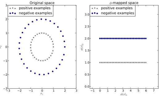
strat-Figure 1.1 – Left: An example dataset for an SVM. Right: The same dataset transformed by (x), where is conversion to polar coordinates.
can reduce both overfitting and underfitting. However, it can be difficult to explicitly design good functions . Feature learning refers to learning the feature mapping . All of the work in this thesis employs this strategy in one way or another.
As an example, consider fitting a linear SVM to the dataset depicted in Fig1.1. In the original space, the SVM cannot represent the right decision boundary. In the transformed space, it is easy to linearly separate the data.
In this example, was mostly helpful because it overcame a problem with the linear SVM’s representational capacity–even with infinite data, the SVM simply has no way of specifying the right decision boundary to separate the data. Most practical applications of feature learning also aim to improve statistical efficiency.
Many feature learning algorithms are based on unsupervised learning, and can learn a reasonably useful mapping without any labeled data. This allows hy-brid learning systems that can improve performance on supervised learning tasks by learning features on unlabeled data. One of the main reasons this approach is beneficial is that unlabeled data is usually more abundant. For example, an unsu-pervised learning algorithm trained on a large amount of images of cats and cars
“has wheels.” A classifier trained with these high-level input features then needs few labeled examples in order to generalize well.
Even when all of the available examples are labeled, training the features to model the input can provide some regularization.
Unsupervised feature learning is also useful because it allows the model to be split into pieces and trained one component at a time, even if each individual component cannot be meaningfully associated with an output target. For example, if we divide a 32⇥ 32 pixel image of a cat into a collection of small 6 ⇥ 6 pixel image patches, many of these patches do not contain any portion of the cat at all and those that do contain some portion of the cat probably do not contain enough information to identify it. We therefore cannot associate each image patch with a label, so supervised learning cannot make progress with the input divided up in this way. Unsupervised learning can still learn good descriptions of each image patch, allowing us to learn thousands of features per image patch. When extracted at all locations in the image, this corresponds to millions of features per image. Learning these millions of features on a per-patch basis greatly reduces the computational cost of training such a system. This patch-based learning approach has been used in several practical applications (Lee et al.,2009;Coates et al.,2011) and is exploited in this thesis.
A closely related idea to feature learning is deep learning (Bengio,2009). In deep learning, the feature extractor is formed by composing several simpler mappings:
(x) = (L)( (L 1)(. . . (1)(x)))
where L is the total number of mappings. Each mapping (i) is known as a layer.
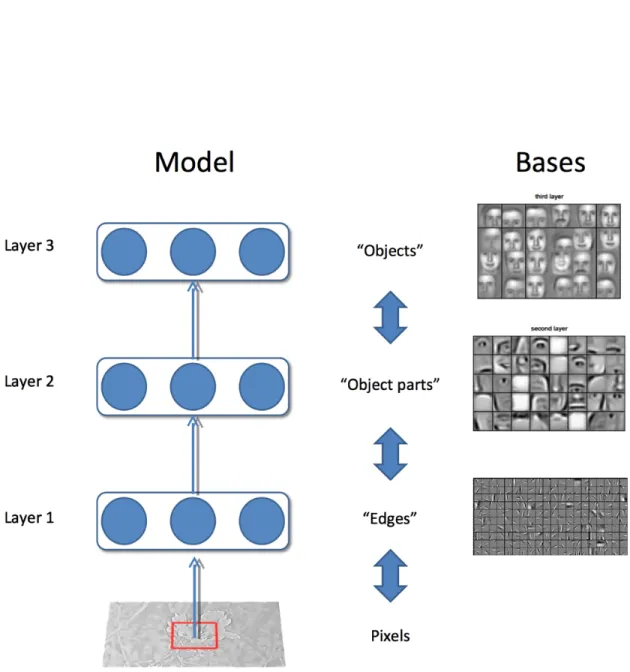
The composite feature extractor is considered “deep” because the computational graph describing it has several of these layers. Each layer of a deep learning system can be thought of as being analogous to a line of code in a program–each layer references the results of earlier layers, and complicated tasks can be accomplished by running multiple simple layers in sequence. For example, see Fig. 1.2.
Deep learning was popularized by the success of deep belief networks (Hinton et al., 2006), stacked autoencoders (Bengio et al., 2007), and stacked denoising autoencoders (Vincent et al.,2008). In these approaches to deep learning, each
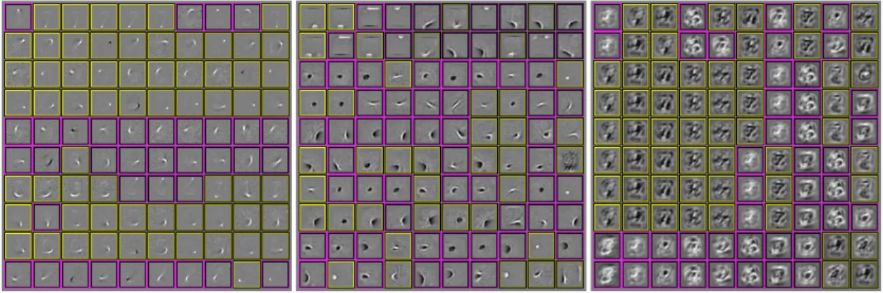
sub-Figure 1.2 – Deep learning example: When trained on images, the first layer of a deep learning system operates on the pixels and usually extracts some sort of edges from the image. The second layer operates on this representation in terms of edges and might extract small object parts that can be described as collections of small numbers of edges. The third layer operates on this representation in terms of object parts and might extract entire objects that can be described as collections of small numbers of object parts. The exact results depend on the algorithm employed, model architecture, and formatting of the dataset. (This image was joint work with Honglak Lee and Andrew Saxe, originally prepared for an oral presentation of (Goodfellow et al.,2009))
This pretraining is usually followed by joint fine-tuning of the entire system. Since this style of deep learning system is formed by composing shallow learn-ers, a popular form of deep learning research is devising new shallow learners. Some examples of recent work in developing shallow learners for feature learn-ing includes work with sparse codlearn-ing (Raina et al., 2007), restricted Boltzmann machines (RBMs) (Hinton et al., 2006; Courville et al., 2011a), the aforemen-tioned autoencoder-based methods, and hybrids of autoencoders and sparse cod-ing (Kavukcuoglu et al., 2010a). The spike-and-slab sparse coding work we intro-duce in chapter 5 can be seen as a continuation of this line of research.
Other approaches to deep learning involve training the entire deep learning system simultaneously. This is the approach we use in the remainder of this thesis.
2
Structured Probabilistic
Models
Chapter 1 presented some of the basic ideas of probabilistic modeling with maximum likelihood estimation. This chapter explores these ideas in greater depth, applying maximum likelihood estimation to more complicated models that require us to introduce approximations.
Sections2.1and2.2describe two ways of representing structure in a probabilistic model. Viewing probabilistic models as containing simplifying structure is a crucial cognitive tool that motivates design choices throughout the rest of this thesis. Section 2.3 explains a basic design choice about how to represent complicated interactions between multiple units.
Section 2.4 explains how to train models for which the likelihood cannot be computed using sampling-based approximations to the gradient of the log likeli-hood. Other approximate methods of training are possible for these models but the strategies detailed in this section are the ones that are used in this thesis.
Section2.5, demonstrates how models with an intractable posterior distribution over their latent variables can be trained using variational approximations. Again, other approximations are possible, so the presentation here focuses on the methods actually used in the present work.
Finally, I’ll discuss combining both forms of approximation in section 2.6.
2.1
Directed models
In general, a probability distribution over a vector-valued variable x repre-sents probabilistic interactions between all of the variables. Suppose that x 2 {1, . . . , k}n. To parameterize a fully general P (x) on discrete data like this is
of the outcome space, with the probability of the last entry determined by the constraint that a probability distribution sum to 1)
Fortunately, most probability distributions we actually work with in practice do not involve all possible interactions between all possible variables. Many variables interact with each other only indirectly. This allows us to greatly simplify our representation of the distribution.
Probabilistic models that exploit this idea are called structured probabilistic models, because they represent the variables as belonging to a structure that re-stricts their ability to interact directly. Structure enables a model to do its job with fewer parameters, thus reducing the computational cost of storing it and increas-ing its statistical efficiency. It also reduces the computational cost of performincreas-ing operations like computing marginal or conditional distributions over subsets of the variables (Koller and Friedman,2009).
A common form of structured probabilistic model is the Bayesian network (Pearl, 1985). A Bayesian network is defined by a directed acyclic graph G whose vertices are the random variables in the model, and a set of local conditional prob-ability distributions p(xi | PaG(xi)) where PaG(xi) returns the parents of xi inG.
The probability distribution over x is given by p(x) = ⇧ip(xi | PaG(xi)).
So long as each variable has few parents in the graph, the distribution can be represented with very few parameters. Simple restrictions on the graph structure can also guarantee that operations like computing marginal or conditional distri-butions over subsets of variables are efficient.
2.2
Undirected models
Some interactions between variables may not be well-captured by local con-ditional probability distributions. For example, when modeling the pixels in an image, there is no clear reason for one pixel to be a parent of the other; their
A Markov network (Kindermann,1980) is a structured graphical model defined on an undirected graphG. For each clique C in the graph, a factor (C) measures the affinity of the variables in that clique for being in each of their possible states. The factors are constrained to be non-negative. Together they define an unnormalized probability distribution
˜
p(x) = ⇧C2G (C).
The unnormalized probability distribution is efficient to work with so long as all the cliques are small.
Obtaining the normalized probability distribution may be costly. To do so, one must compute the partition function Z (though Z is conventionally written without arguments, it is in fact a function of whatever parameters govern each of the functions). Since
Z = Z
x
˜ p(x)dx
it may be intractable to compute for high-dimensional x, depending on the structure of G and the functional form of the s.
Many interesting theoretical results about undirected models depend on the assumption that 8x, ˜p(x) > 0. A convenient way to enforce this to use an energy-based model (EBM) where
˜
p(x) = exp( E(x))
and E(x) is known as the energy function. This can still be interpreted as a standard Markov network; the exponentation makes each term in the energy func-tion correspond to a factor for a di↵erent clique. The sign isn’t strictly necessary from a computational point of view (and some machine learning researchers have tried to do without it, e.g. (Smolensky, 1986)). It is a commonly used conven-tion inherited from statistical phyiscs, along with the terms “energy funcconven-tion” and “partition function.”
Some results in this chapter are presented in terms of energy-based models. For these results, the theory doesn’t hold if ˜p(x) = 0 for some x. Note that a directed graphical model may be encoded as an energy-based model so long as this condition
2.2.1
Sampling
Drawing a sample x from the probability distribution p(x) defined by a struc-tured model is an important operation. We briefly describe how to sample from directed models and EBMs here. For more detail, see (Koller and Friedman,2009). Sampling from a directed model is straightforward, assuming that one can sam-ple from each of the conditional probability distributions. The procedure used in this case is called ancestral sampling. One simply draws samples of each of the variables in the network in an order that respects the network topology, i.e., before sampling a variable xi from P (xi | Paxi), sample each of the members of Paxi. This
defines an efficient means of sampling all variables with a single pass through the network.
Sampling from an EBM is not straightforward. Suppose we have an EBM defining a distribution p(a, b). In order to sample a, we must draw it from p(a| b), and in order to sample b, we must draw it from p(b | a). This “chicken and egg” problem means we can no longer use ancestral sampling. Since G is no longer directed and acyclical, we don’t have a way of ordering the variables such that every variable can be sampled given only variables that come earlier in the ordering.
It turns out that we can sample from an EBM, but we can not generally do so with a single pass through the network. Instead we need to sample using a Markov chain. A Markov chain is defined by a state x and a transition distribution T (x0 | x). Running the Markov chain means repeatedly updating the state x to a value x0 sampled from T (x0 | x).
Under certain distributions, a Markov chain is eventually guaranteed to draw x from an equilibrium distribution ⇡(x0), defined by the condition
8x0, ⇡(x0) = X
x
T (x0 | x)⇡(x).
This condition guarantees that repeated applications of the transition sampling procedure don’t change the distribution over the state of the Markov chain. Run-ning the Markov chain until it reaches its equilibrium distribution is called “burRun-ning in” the Markov chain.
same distribution, they are highly correlated with each other, so to obtain multiple independent samples one should run the Markov chain for several steps between collecting each sample. Markov chains tend to get stuck in a single mode of ⇡(x) for several steps. The speed with which a Markov chain moves from mode to mode is called its mixing rate. Since burning in a Markov chain and getting it to mix well may take several sampling steps, sampling correctly from an EBM is still a somewhat costly procedure.
Of course, all of this depends on ensuring ⇡(x) = p(x) . Fortunately, this is easy so long as p(x) is defined by an EBM. The simplest method is to use Gibbs sampling, in which sampling from T (x0 | x) is accomplished by selecting one variable x
i and
sampling it from p conditioned on its neighbors in G. It is also possible to sample several variables at the same time so long as they are conditionally independent given all of their neighbors.
2.3
Latent variables
Most of this thesis concerns models that have two types of variables: observed or “visible” variables v and latent or “hidden” variables h. v corresponds to the variables actually provided in the design matrix X during training. h consists of variables that are introduced to the model in order to help it explain the structure in v. Generally the exact semantics of h depend on the model parameters and are created by the learning algorithm. The motivation for this is twofold.
2.3.1
Latent variables versus structure learning
Often the di↵erent elements of v are highly dependent on each other. A good model of v which did not contain any latent variables would need to have very large numbers of parents per node in a Bayesian network or very large cliques in a Markov network. Just representing these higher order interactions is costly–both in a computational sense, because the number of parameters that must be stored in memory scales exponentially with the number of members in a clique, but also in a statistical sense, because this exponential number of parameters requires a wealth
There is also the problem of learning which variables need to be in such large cliques. An entire field of machine learning called structure learning is devoted to this problem . Most structure learning techniques involve fitting a model with a specific structure to the data, assigning it some score that rewards high training set accuracy and penalizes model complexity, then greedily adding or subtracting an edge from the graph in a way that is expected to increase the score. See (Koller and Friedman, 2009) for details of several approaches.
Using latent variables mostly avoids the problem of learning structure. A fixed structure over visible and hidden variables can use direct interactions between visible and hidden units to impose indirect interactions between visible units. Using simple parameter learning techniques we can learn a model with a fixed structure that imputes the right structure on the marginal p(v). Of course, one still has the problem of determining the amount of latent variables and their connectivity, but it is usually not as important to determine the absolutely optimal model architecture when using latent variables as when using structure learning on fully observed models. Usually, in the context of deep learning and latent variable models, the architecture is controlled by a small number of hyperparameters, which are searched relatively coarsely.
2.3.2
Latent variables for feature learning
Another advantage of using latent variables is that they often develop useful semantics. As discussed in section 1.3, the mixture of Gaussians model learns a latent variable that corresponds to which category of examples the input was drawn from. Other more sophisticated models with more latent variables can create even richer descriptions of the input. Most of the approaches mentioned in section 1.4 accomplish feature learning by learning latent variables. Often, given some model of v and h, it turns out that E[h | v] or argmaxhp(h, v) is a good feature mapping
2.4
Stochastic approximations to maximum
likelihood
Consider an energy-based model p(v, h) = 1
Zexp( E(v, h)).
Suppose that the partition function Z cannot be computed. This model may still be useful. As explained in section 2.2.1, one can still draw samples from this model, perhaps even efficiently. One might also be able to compute the ratio of the probability of two events, p(v, h)/p(v0, h0), or the posterior p(h| v), which as shown in 2.3 could be useful as a set of features to describe v.
Given that such a model is useful, learning one is a desirable capability. How-ever, our primary method of learning models is maximum likelihood estimation. As seen in section 1.1.3, this involves computing
r✓log p(v).
Unfortunately, if we expand the definition of p(v), we see that this expression contains Z:
r✓log ˜p(v) r✓log Z.
Since Z is intractable, there doesn’t seem to be much hope of computing r✓log Z.
Fortunately, so long as Leibniz’s rule applies, a sampling trick can approximate the gradient:
@ @✓i log Z = @ @✓i log Z v Z h ˜ p(v, h)dhdv = @ @✓i R v R hp(v, h)dhdv˜ R v R hp(v, h)dhdv˜ = 1 Z Z v Z h @ @✓i exp( E(v, h))dhdv = 1 Z Z v Z h exp( E(v, h)) @ @✓i E(v, h)dhdv = Ev,h[ @ @✓i E(v, h)]
The expectation can be approximated by drawing samples of v and h, but this of course raises the question of how to set up the Markov chain in a way that yields a good approximation and is efficient.
The naive approach is to initialize a new Markov chain and run it to its equilib-rium distribution on every step of stochastic gradient ascent. Unfortunately, that is too expensive.
One solution to this problem is contrastive divergence (CD-k) (Hinton, 2002). This approach makes use of several Markov chains in parallel, one per example in the minibatch. At each learning step, each Markov chain is initialized with the corresponding data example and run for k steps. Typically k = 1. Clearly this approach only explores parts of space that are near the data points. This procedure generally results in the model’s distribution having about the right shape near the data points, but the model may inadvertently learn to represent other modes far from the data.
Another approach is known alternatively as stochastic maximum likelihood (SML) (Younes,1998) or persistent contrastive divergence (PCD) (Tieleman, 2008). This approach also makes use of parallel Markov chains but each is initialized only once, at the start of training. The state of each chain is sampled once per gradient
h
1
h
2
h
3
v
1
v
2
v
3
h
4
Figure 2.1 – An example RBM drawn as a Markov network
even though that equilibrium distribution is continually changing. The advantage of SML over CD is that each Markov chain is updated for several steps, and con-sequently should explore all of the model’s modes. This enables SML to suppress modes that are far from the data that CD might overlook.
2.4.1
Example: The restricted Boltzmann machine
The restricted Boltzmann machine (RBM) (Smolensky,1986) is an example of a model that has intractable Z (Long and Servedio,2010) yet may be trained using the techniques described in this section (Hinton, 2002).
It is an energy-based model with binary visible and hidden units. Its energy function is
E(v, h) = b>v c>h v>Wh
where b, c, and W are unconstrained, real-valued, learnable parameters. The model is depicted graphically in Fig. 2.1. As this figure makes clear, an important aspect of this model is that there are no direct interactions between any two visible units or between any two hidden units (hence the “restricted”; a general Boltzmann machine may have arbitrary connections).
The restrictions on the RBM structure yield the nice properties
p(v | h) = ⇧ip(vi | h).
The individual conditionals are simple to compute as well, for example p(hi = 1| v) = v>Wi+ bi
where is the logistic sigmoid function.
Together these properties allow for efficient block Gibbs sampling, alternating between sampling all of h simultaneously and sampling all of v simultaneously.
Since the energy function itself is just a linear function of the parameters, it is easy to take the needed derivatives. For example,
@ @Wij
E(v, h) = vihj.
These two properties–efficient Gibbs sampling and efficient derivatives– make it possible to train the RBM with stochastic approximations tor✓log Z.
2.5
Variational approximations
Another common difficulty in probabilistic modeling is that for many models the posterior distribution p(h| v) is infeasible to compute or even represent. Alter-nately, it may be infeasible to take expectations with respect to this distribution.
This poses problems for our goal outlined in section 2.3.2 of using E[h | v] as features. It also usually means that maximum likelihood estimation is infeasible. As shown in (Neal and Hinton,1999), maximizing p(v) is equivalent to maximizing
Eh⇠P (h|v)log P (v, h).
Fortunately, variational approximations provide a solution to both of these dif-ficulties.
2.5.1
Variational learning
For any distribution Q(h), the log likelihood may be decomposed (Neal and Hinton,1999) into two terms.
log p(v) = DKL(Q(h)kp(h | v)) + L(v, Q).
Here, DKL is the Kullback-Leibler (KL) divergence (Kullback and Leibler,1951)
and L is the negative variational free energy. The KL divergence is guaranteed to be non-negative, so this decomposition proves
log p(v) L(v, Q).
L(v, Q) is thus a lower bound on the log likelihood. The KL divergence measures the di↵erence between two distributions, and goes to 0 when the two distributions are the same. Thus this lower bound is tight when Q(h) = P (h| v). Consequently, one can maximize L(v, Q) as a proxy for log p(v). Note that this maximization will involve modifying both the distribution Q (to make the lower bound tighter) and the parameters controlling p (to optimize the model using the bound).
In order to maximize L, let’s examine its functional form:
L(v, Q) = Eh⇠Q[log P (v, h)] + HQ(h)
where HQ(h) is the Shannon entropy (Cover,2006) of h under Q.
Since computingL(v, Q) involves taking an expectation with respect to Q, it is necessary to restrict Q in order to make the expectation tractable. A particularly elegant way to restrict Q is to require it to take the form of a graphical model with a specific graph structure G (Saul and Jordan, 1996). A common approach is to use the mean field approximation
Q(h) = ⇧iQ(hi)
which corresponds to aG with no edges. So long as inference in Q remains tractable, one can obtain better approximations by using a more complicated G. This ap-proach is known as structured variational approximation.
2.5.2
Variational inference
A common operation is to compute the Q that minimizes DKL(Q(h)kP (h | v)).
This is necessary for extracting featuresE[h | v]. It is also a common inner-loop to variational learning algorithms which alternate between optimizing L(v, Q) with respect to Q and optimizing it with respect to the model parameters.
This operation is called variational inference (Koller and Friedman, 2009) be-cause in the general case it involves solving a calculus of variations problem. Calcu-lus of variations is the study of optimizing functionals. A functional is a mapping much like a function, except that a functional takes a function as its input. In variational inference, the functional being minimized is the KL divergence. The function being optimized is the distribution Q. Note that in the special case where none of the h variables is continuous, Q is merely a vector and may be optimized with traditional calculus techniques.
Usually variational inference involves using calculus of variations to find the functional form of Q, followed by an iterative procedure to find the parameters of Q. Consider the following example from (Bishop, 2006).
Suppose h2 R2 and p(h| v) = N (h | µ, 1) (for the purpose of simplicity, in
this example, the hidden units do not actually interact with the visible units). Constrain Q with the mean field assumption Q(h) = Q(h1)Q(h2). Using
calcu-lus of variations one may then show
Q(hi) = N (hi | ˆhi, 1/ i,i).
In other words, the fact that p(h | v) is jointly Gaussian implies that the correct Q is also Gaussian. We never assumed that Q was Gaussian, only that it was factorial. The Gaussian nature of Q had to be derived via calculus of variations. There is still an unknown: the mean of Q, ˆh. This is an example of a variational parameter, a parameter controlling Q that cannot be found analytically. These parameters must be obtained by an iterative optimization procedure. Gradient descent would work, but is a slow and expensive procedure to use in the inner loop of a learning algorithm. Typically it is faster to optimize these parameters by iterating between fixed point equations.