HAL Id: hal-01887266
https://hal.archives-ouvertes.fr/hal-01887266v2
Submitted on 24 Dec 2018
HAL is a multi-disciplinary open access
archive for the deposit and dissemination of sci-entific research documents, whether they are pub-lished or not. The documents may come from teaching and research institutions in France or
L’archive ouverte pluridisciplinaire HAL, est destinée au dépôt et à la diffusion de documents scientifiques de niveau recherche, publiés ou non, émanant des établissements d’enseignement et de recherche français ou étrangers, des laboratoires
Polynomial-time Recognition of 4-Steiner Powers
Guillaume Ducoffe
To cite this version:
Guillaume Ducoffe. Polynomial-time Recognition of 4-Steiner Powers. [Research Report] University of Bucharest, Faculty of Mathematics and Computer Science; National Institute for Research and Development in Informatics, Romania. 2018. �hal-01887266v2�
Polynomial-time Recognition of 4-Steiner Powers
Guillaume Ducoffe1,2,3
1National Institute for Research and Development in Informatics, Romania
2The Research Institute of the University of Bucharest ICUB, Romania 3University of Bucharest, Faculty of Mathematics and Computer Science, Romania
Abstract
The kth-power of a given graph G “ pV, Eq is obtained from G by adding an edge between
every two distinct vertices at a distance ď k in G. We call G a k-Steiner power if it is an induced subgraph of the kth-power of some tree. Our main contribution is a polynomial-time recognition algorithm of 4-Steiner powers, thereby extending the decade-year-old results of (Lin, Kearney and Jiang, ISAAC’00) for k “ 1, 2 and (Chang and Ko, WG’07) for k “ 3.
A graph G is termed k-leaf power if there is some tree T such that: all vertices in V pGq are leaf-nodes of T, and G is an induced subgraph of the kth-power of T. As a byproduct of our main result, we give the first known polynomial-time recognition algorithm for 6-leaf powers.
1
Introduction
A basic problem in computational biology is, given some set of species and a dissimilarity measure in order to compare them, find a phylogenetic tree that explains their respective evolution. Namely, such a rooted tree starts from a common ancestor and branches every time there is a separation between at least two of the species we consider. In the end, the leaves of the phylogenetic tree should exactly represent our given set of species. This problem was brought to Graph theory under several disguises but, unfortunately, several of these formulations are NP-hard to solve [BFW92, Ste92]. We here study a related problem whose complexity status remains open. Specifically, a common assumption in the literature is that our dissimilarity measure can only tell us whether the separation between two given species has occurred quite recently. Let G “ pV, Eq be a graph whose vertices are the species we consider and such that an edge represents two species with a quite “close” common ancestor according to the dissimilarity measure. Given some fixed k ě 1, we ask whether there exists some tree T whose leaf-nodes are exactly V and such that there is an edge uv in E if and only if the two corresponding nodes in T are at a distance ď k. This is called the k-Leaf Power problem [NRT02].
The structural properties of k-leaf powers (i.e., graphs for which a tree as above exists) have been intensively studied [BPP10, BH08, BHMW10, BL06, BLS08, BLR09, WB09, CFM11, DGHN06, DGHN08, DGN05, KLY06, KKLY10, Laf17, NR16, Rau06]. From the algorithmic point of view, k-leaf powers are a subclass of bounded clique-width graphs, and many NP-hard problems can be solved efficiently for these graphs [FMR`08, GW07]. However, the computational complexity
of recognizing k-leaf powers is an open problem. Very recently, parameterized algorithms were proposed for every fixed k on the graphs with degeneracy at most d, where the parameter is
k ` d [EH18]. Without this additional restriction on the degeneracy of the graphs, polynomial-time recognition algorithms are known only for k ď 5 [BL06, BLS08, CK07]. It is noteworthy that every algorithmic improvement for this problem has been incredibly hard to generalize to larger values of k. We contribute to this frustrating chain of improvements by providing the first known polynomial-time recognition algorithm for 6-leaf powers.
Theorem A. There is a polynomial-time algorithm that given a graph G “ pV, Eq, correctly decides whether G is a 6-leaf power (and if so, outputs a corresponding tree T).
Several variations of k-leaf powers were introduced in the literature [BLR10, BW10, CK07, HT10, JKL00]. In this work, we consider k-Steiner powers: a natural relaxation of k-leaf powers where the vertices in the graph may also be internal nodes in the tree T. Interestingly, for every k ě 3, the notions of k-leaf powers and pk ´ 2q-Steiner powers are equivalent for a twin-free graph. The latter implies a linear-time reduction from k-Leaf Power to pk´2q-Steiner Power [BLS08]. Furthermore, there exist polynomial-time recognition algorithms for k-Steiner powers, for every k ď 3 [CK07, JKL00]. As our main contribution in the paper we obtain the first improvement on the recognition of k-Steiner powers in a decade. Specifically we prove that there is a polynomial-time recognition algorithm for the 4-Steiner powers.
Theorem B. There is a polynomial-time algorithm that given a graph G “ pV, Eq, correctly decides whether G is a 4-Steiner power (and if so, outputs a corresponding tree T).
Note that Theorem A follows from the combination of Theorem B with the aforementioned reduction from k-Leaf Power to pk ´ 2q-Steiner Power [BLS08]. Hence, the remaining of this paper is devoted to a polynomial-time solution for 4-Steiner Power. We think that our general approach (presented next) could be generalized to larger values of k. However, this would first require to strenghten the structure theorems we use in this paper (and probably to find less intricate proofs for some of our intermediate statements).
Before we can introduce our technical contributions in this paper, we must explain in Sec. 1.1 the dynamic programming approach behind the k-Steiner power recognition algorithms, for k ď 3, and why it is so hard to apply this approach to 4-Steiner Power. Doing so, we identify Obstacles O1 and O2 as the two main issues to fix in order to prove Theorem B. Then in Sec. 1.2, we briefly summarize our proposed solutions for Obstacles O1 and O2 while presenting the organization of the technical sections of this paper.
1.1 The difficulties of a dynamic programming approach
We refer to Sec. 2 for any undefined graph-theoretic terminology in this introduction. In what follows we give a high-level overview of our approach, that we compare to prior work on k-Steiner Power and k-Leaf Power. As our starting point we restrict our study to chordal graphs and strongly chordal graphs, that are two well-known classes in algorithmic graph theory of which k-Steiner powers form a particular subclass [ABNT16]. Doing so, we can use various properties of these classes of graphs such as: the existence of a tree-like representation of chordal graphs, that is called a clique-tree [BP93] and is commonly used in the design of dynamic programming algorithms on this class of graphs; and an auxiliary data structure which is called “clique arrangement” and is polynomial-time computable on strongly chordal graphs [NR16]. Roughly, this clique arrangement encodes all possible intersections of a subset of maximal cliques in a graph. It is worth noticing
that clique arrangements were introduced in the same paper as leaf powers, under the different name of “clique graph” [NRT02].
Our first result is that every maximal clique, minimal separator and, more generally, any inter-section of maximal cliques in a k-Steiner power must induce a subtree with very specific properties – detailed next – of the tree T we aim at computing. This result – that extends to any k the struc-tural results that were presented in [CK07] for k ď 3 – is a prerequisite for the design of a dynamic programming algorithm on a clique-tree. Unfortunately, as the value of k increases it becomes more and more difficult to derive from such structural results a polynomial-time recognition algorithm for k-Steiner powers. Our proposed solutions for k “ 4 are quite different from those used in the previous works on k-Steiner powers [CK07, JKL00] which results in an embarrassingly long and intricate proof.
To give a flavour of the difficulties we met, we consider the following common situation in a dynamic programming algorithm on chordal graphs. Given a graph G “ pV, Eq, let S be a minimal separator of G and C be a full component of GzS (i.e., such that every vertex in S has a neighbour in C). If G is a k-Steiner power then, so must be the induced subgraph GrC Y Ss. We want to store the partial solutions obtained for GrC Y Ss, as at least one of them should be extendible to all of G (otherwise, G is not a k-Steiner power). However, for doing so efficiently we must overcome the following two obstacles:
- There may be exponentially many partial solutions already when GrC Y Ss is a complete subgraph and k ě 3. Therefore, we cannot afford to store all possible solutions explicitly. Nevertheless it seems at the minimum we need to keep the part of these solutions which contains S: in order to be able to check later whether the solutions found for GrC Y Ss can be extended to all of G. We will prove in this paper that such a part TxSy of the partial solutions is a subtree of diameter at most k ´ 1, and so, there may be exponentially many possibilities to store whenever k ě 4.
Obstacle O1. Decrease the number of possibilities to store for TxSy to a polynomial. - Furthermore, since there can be no edge between C and V z pC Y Sq, the tree T that we want
to compute for G must satisfy that all vertices in C stay at a distance ě k ` 1 from all vertices in V zpS Y Cq. In order to ensure this will be the case, we wish to store a “distance profile” pdistTpr, CqqrPV pTxSyq in the encoding of all the partial solutions found for GrC Y Ss.
Storing this information would result in a combinatorial explosion of the number of possible encodings, even if there are only a few possibilities for the subtree TxSy. Chang and Ko proposed two nice “heuristic rules” in order to overcome this distance issue for k “ 3 [CK07]. Unfortunately, these rules do not easily generalize to larger values of k.
Obstacle O2. For any fixed TxSy, decrease the number of possibilities to store for the “dis-tance profiles” to a polynomial.
In order to derive a polynomial-time algorithm for the case k “ 4, we further restrict the structural properties of the “useful” partial solutions we need to store. This is done by carefully analysing the relationships between the structure of these solutions and the intersections between maximal cliques in the graph. Perhaps surprisingly, we need to combine these stronger properties on the partial solutions with several other tricks so as to bound the number of partial solutions that we need to store by a polynomial (e.g., we also impose local properties on the clique-tree we use, and we introduce a new greedy selection procedure based on graph matchings).
1.2 Organization of the paper
We give the required graph-theoretic terminology for this paper in Section 2. We emphasize on Section 2.3: where we also provide a more detailed presentation of our algorithm, as a guideline for all the other sections.
Given a k-Steiner power G, let us call k-Steiner root a corresponding tree T. In Sections 3 and 4 we present new results on the structure of k-Steiner roots that we use in the analysis of our algorithm. Specifically, we show in Section 3 that any intersection of maximal cliques in a graph G must induce a particular subtree in any of its k-Steiner roots T where no other vertex of G can be present. Furthermore, the inclusion relationships between these “clique-intersections” in G are somewhat reflected by the diameter of their corresponding subtrees in T. An intriguing consequence of our results is that, in any k-Steiner power, there can be no chain of more than k minimal separators ordered by inclusion. This slightly generalizes a similar result obtained in [NRT02] for k-leaf powers.
Then, we partly complete this above picture in Section 4 for the case k “ 4. For every clique-intersection X in a chordal graph G, we classify the vertices in X into two main categories: “free” and ”constrained”, that depend on the other clique-intersections these vertices are contained into. Our study shows that “free” vertices cause a combinatorial explosion of the number of partial solutions we should store in a naive dynamic programming algorithm. However, on the positive side we prove that there always exists a “well-structured” 4-Steiner root where such free vertices are leaves with very special properties. This result will be instrumental in ruling out Obstacle O1. Sections 5, 6, 7 and 8 are devoted to the main steps of the algorithm. We start presenting a constructive proof of a rooted clique-tree with quite constrained properties in Section 5. Roughly we carefully control the ancestor/descendant relationships between the edges that are labelled by different minimal separators of the graph. These technicalities are the cornerstone of our approach in Section 3 in order to bound the number of “distance profiles” which we need to account in our dynamic programming (cf. Obstacle O2).
Then in Section 6, we completely rule out Obstacle O1 — in fact, we solve a more general subproblem. For that, let TG be the rooted clique-tree of Section 5. Recall that the maximal
cliques and the minimal separators of G can be mapped to the nodes and edges of TG, respectively.
We precompute by dynamic programming, for every node and edge in TG, a family of all the
potential subtrees to which the corresponding clique-intersection of G could be mapped in some “well-structured” 4-Steiner root of G. Of particular importance is Section 6.1, where we give a polynomial-time algorithm in order to generate all the candidate subtrees any minimal separator of the graph can induce in its 4-Steiner roots. The result is then easily extended to the maximal cliques that appear as leaves in our clique-tree (Section 6.2). Correctness of these two first parts follows from Sec. 4. Finally, in Section 6.3 we give a more complicated representation of a family of potential subtrees TxKiy for all the other maximal cliques Ki. This part is based on a careful
analysis of clique-intersections in Ki and several additional tricks. Roughly, our representation in
Sec. 6.1 is composed of partially constructed subtrees and of “problematic” subsets that need to be inserted to these subtrees in order to complete the construction. The exact way these insertions must be done is postponed until the very end of the algorithm (Sec. 8).
Section 7 is devoted to the “distance profiles” of partial solutions and how to overcome Ob-stacle O2. Specifically, instead of computing partial solutions at each node of the clique-tree and storing their encodings, we rather pre-compute a polynomial-size subset of imposed encodings for
each node. Then, the problem becomes to decide whether given such an imposed encoding, there exists a corresponding partial solution. We formalize our approach by introducing an intermediate problem where the goal is to compute a 4-Steiner root with additional constraints on its structure and the distances between some sets of nodes.
Finally, we detail in Section 8 the resolution of our intermediate problem using an ad hoc data structure, thereby completing the presentation of our algorithm. An all new contribution in this part is a greedy procedure, based on Maximum-Weight Matching, in order to ensure some distances’ constraints are satisfied by the solutions we generate during the algorithm. Interestingly, this procedure is very close in spirit to the implementation of the alldifferent constraint in constraint programming [R´eg94].
Due to the intricacy of our proofs we gave up optimizing the runtime of our algorithm. We will only provide enough arguments in order to show it is polynomial.
We end up this paper in Section 9 with some ideas for future work.
2
Preliminaries
We refer to [BM08] for any undefined graph terminology. All graphs in this study are finite, simple (hence, with neither loops nor multiple edges), unweighted and connected – unless stated otherwise. Given a graph G “ pV, Eq, let n :“ |V | and m :“ |E|. The neighbourhood of a vertex v P V is defined as NGpvq :“ tu P V | uv P Eu. By extension, we define the neighbourhood of a set S Ď V
as NGpSq :“ p
Ť
vPSNGpvqq zS. The subgraph induced by any subset U Ď V is denoted by GrU s.
For every u, v P V , we denote by distGpu, vq the minimum length (number of edges) of a
uv-path. The eccentricity of vertex v is defined as eccGpvq :“ maxuPV distGpu, vq. The radius
and the diameter of G are defined, respectively, as radpGq :“ minvPV eccGpvq and diampGq :“
maxvPV eccGpvq. We denote by C pGq the center of G, a.k.a. the vertices with minimum eccentricity.
2.1 Problems considered
The kth-power of G, denoted Gk has same vertex-set V as G and edge-set Ek :“ tuv | 0 ă
distGpu, vq ď ku. We call G a k-Steiner power if there is some tree T such that G is an induced
subgraph of Tk. Conversely, T is called a k-Steiner root of G. If in addition, G has a k-Steiner root where all vertices in V are leaves (degree-one nodes) then, we call G a k-leaf power.
Problem 1 (k-Steiner Power). Input: A graph G “ pV, Eq. Output: Is G a k-Steiner power? Problem 2 (k-Leaf Power). Input: A graph G “ pV, Eq. Question: Is G a k-leaf power?
Theorem 2.1 ( [BLS08]). There is a linear-time reduction from k-Leaf Power to pk´2q-Steiner Power for every k ě 3.
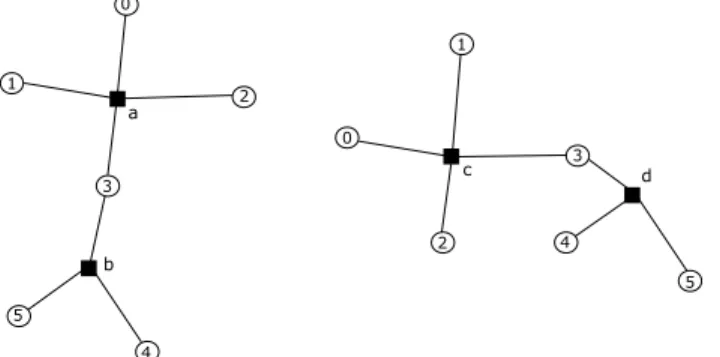
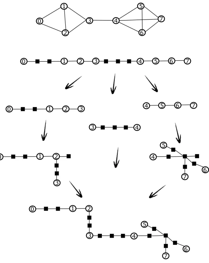
0 0 1 1 2 2 3 3 4 4 5 5 a b c d
Figure 1: Two Steiner-equivalent trees. Cycles and rectangles represent real and Steiner nodes, respectively.
If T is any k-Steiner root of G then, nodes in V pGq are called real, whereas nodes in V pTqzV pGq are called Steiner. We so define, for any S Ď V pTq (for any subtree T1
Ď T, resp.): RealpSq :“ S X V pGq and SteinerpSq :“ SzV pGq
(we define RealpT1
q :“ RealpV pT1qq and SteinerpT1q “ SteinerpV pT1qq, resp.).
Note that throughout all this paper we consider two (sub)trees being equivalent if they are equal up to an appropriate identification of their Steiner nodes, namely (see also Fig. 1):
Definition 2.1. Given G “ pV, Eq, we call any two trees T, T1Steiner-equivalent, denoted T ” GT1,
if and only if RealpTq “ RealpT1q “ S and there exists an isomorphism ι : V pTq Ñ V pT1q such that
ιpvq “ v for any v P S.
Finally, given a node-subset X Ď V pTq, TxXy is the smallest subtree of T such that X Ď V pTxXyq. Note that for a vertex-subset X Ď V , this is the smallest subtree of T such that X Ď RealpTxXyq. Furthermore we observe T rXs Ď TxXy, with equality if and only if T rXs is connected.
2.2 Algorithmic tool-kit: (Strongly) Chordal graphs
Given G “ pV, Eq, we call it a chordal graph if every induced cycle in G is a triangle. If in addition, for every cycle of even length in G, there exists a chord between two vertices at an odd distance (ą 1) apart from each other in the cycle then, G is termed strongly chordal. Chordal graphs and strongly chordal graphs can be recognized in Opmq-time and Opm log nq-time, respectively [PT87, RTL76].
The following property is well-known:
Theorem 2.2 ( [ABNT16]). For every k ě 1, every k-Steiner power is a strongly chordal graph. Minimal separators and Clique-tree. Our main algorithmic tool in this paper is a clique-tree of G, defined as a tree TGwhose nodes are the maximal cliques of G and such that for every v P V ,
the maximal cliques containing v induce a subtree of TG.
Theorem 2.3 ( [BP93]). A graph G “ pV, Eq is chordal if and only if it has a clique-tree. Moreover if G is chordal then, we can construct a clique-tree for G in Opmq-time.
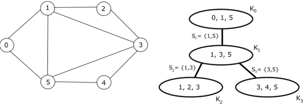
1 0 2 3 4 5 1, 2, 3 3, 4, 5 1, 3, 5 0, 1, 5 K K K K 0 1 2 3 S = {1,5} S = {1,3} S = {3,5} 1 2 3
Figure 2: A chordal graph G (left) and a rooted clique-tree TG (right).
An uv-separator is a subset S Ď V ztu, vu such that u and v are disconnected in GzS. If in addition, no strict subset of S is an uv-separator then, S is a minimal uv-separator. A minimal separator of G is a minimal uv-separator for some u, v P V . It is known that any minimal separator in a chordal graph G is the intersection of two distinct maximal cliques of G. Specifically, the following stronger relationship holds between minimal separators and clique-trees:
Theorem 2.4 ( [BP93]). Given G “ pV, Eq chordal, any of its clique-trees TGsatisfies the following
properties:
• For every edge KiKj P EpTGq, KiX Kj is a minimal separator;
• Conversely, for every minimal separator S of G, there exist two maximal cliques Ki, Kj such
that KiKj P EpTGq and KiX Kj “ S.
Based on the above theorem, we can define ESpTGq :“ tKiKj P EpTGq | KiX Kj “ Su. The
cardinality |ESpTGq | of this subset does not depend on TG [BP93]. We sometimes say that edges
in ESpTGq are labeled by S.
A rooted clique-tree of G is obtained from any clique-tree TGby identifying an arbitrary maximal
clique K0 as its root. Let pKq, Kq´1, . . . , K1, K0q be a postordering of TG (obtained by depth-first
search). For any i ą 0, we define Kppiq as the father node of Ki. The common intersection of Ki
with its father node is the minimal separator Si:“ KiX Kppiq. By convention, we set S0:“ H. We
refer to Fig. 2 for an illustration.
We define TGi as the subtree rooted at Ki, and let Gi be the subgraph induced by all the maximal
cliques in V pTGiq. In particular, we have TG0 “ TG and G0 “ G. We also define Vi :“ V pGiq and
Wi :“ VizSi as shorthands. We will use these above notations for rooted clique-trees throughout
the remaining of our paper.
Clique arrangement. We introduce a common generalization of both maximal cliques and min-imal separators, that will play a key role in our analysis. Specifically, a clique-intersection in G is the intersection of a subset of maximal cliques in G. The family of all clique-intersections in G is denoted by X pGq. For strongly chordal graphs, it is known [NR15] that every clique-intersection is the intersection of at most two maximal cliques. In particular, a (nonempty) clique-intersection of a given strongly chordal G is either: a maximal clique; or a minimal separator; or a weak minimal separator – i.e., whose removal strictly increases the distance between two vertices that remain in
the graph (see [McK11]). We denote by K pGq , S pGq and W pGq the subfamilies of all the maximal cliques, minimal separators and weak minimal separators of G, respectively.
The clique arrangement of G is the inclusion (directed) graph of the clique-intersections of G. That is, there is a node for every clique-intersection, and there is an arc from X to X1 if and only
if we have X Ď X1.
Theorem 2.5 ( [NR15]). Given G “ pV, Eq strongly chordal, the clique arrangement of G can be constructed in Opm log nq-time.
2.3 Highlights of the algorithm
The remaining of the paper is devoted to the proof of Theorem B. By Theorem 2.1, this will also imply Theorem A. We start sketching our algorithm below in order to guide the readers throughout the next sections. Its analysis is based on the structure theorems in Sections 3 and 4. Perhaps surprisingly, we need several tricks in order to keep the running time of this algorithm polynomial. S.0 (Initialization.) Given G “ pV, Eq, we check whether G is strongly chordal. If this is not the case then, by Theorem 2.2, G cannot be a k-Steiner power for any k ě 1, and we stop. Otherwise by Theorem 2.5 we can compute the clique-arrangement of G in polynomial time. Throughout all the remaining sections, we implicitly use the fact that we can access in polynomial time to the clique-arrangement of G. We will also assume in what follows that G is not a complete graph (otherwise, G is trivially a k-Steiner power for any k, and so we also stop in this case).
S.1 (Construction of the clique-tree.) We construct a clique-tree TG of G that we root in some
K0 P K pGq. This clique tree must satisfy very specific properties of which we postpone the
precise statement until Section 5. In order to give the main intuition behind this construction, let us consider an arbitrary maximal clique Ki that is not the root (i.e., i ą 0). Roughly,
we would like to minimize the number of minimal separators in Gi to which the vertices in
Si :“ Ki X Kppiq belong to. Indeed, doing so will help in bounding the number of possible
partial solutions that we will need to consider for processing its father node Kppiq. More
specifically, for every descendant Kj of Ki in TG we would like to impose Sj Ę Si and
Si Ę Sj. However, both objectives are conflicting and so, we need to find a trade-off. The
technical motivations behind our choices will be further explained in Sections 7 and 8. S.2 (Candidate set generation.) This step exploits a result of Section 3 which states that, for
any 4-Steiner root T of G and for any clique-intersection X, we have RealpTxXyq “ X. Equivalently, this result says that in the smallest subtree containing X there can be no other real nodes than those in X. Then, our goal is, for every X P X pGq, to compute a polynomial-size family TX of “candidate subtrees” whose real nodes are exactly X. Intuitively, TX should
contain all possibilities for TxXy in a “well-structured” 4-Steiner root T (such a root must satisfy additional properties given in Sec. 4). Note that in practice, we only need to compute this above family for minimal separators and maximal cliques.
• In Section 6.1 we present an algorithm for computing the collection pTSqSPSpGq for the
minimal separators. This algorithm serves as a brick-basis construction for computing all the other families.
• Then, we consider in Section 6.2 the maximal cliques Ki that are leaf-nodes of TG. We
use the well-known property that all vertices in KizSiare simplicial in order to generalize
the algorithm of the previous section to this new case.
• Finally, we consider the maximal cliques Ki that are internal nodes of TG (Section 6.3).
Unsurprisingly, several new difficulties arise in the construction of TKi. Our bottleneck
is solving the following subproblem: compute (up to Steiner equivalence) all possible central nodes and their neighbourhood in any subtree TxKiy of diameter four. We solved
this subproblem in most situations, e.g., when there is a minimal separator S Ď Ki such
that TxSy must be a bistar (diameter-three subtree). However in some other situations we failed to do so. That left us with some “problematic subsets” called thin branches: with exponentially many possible ways to include them in candidate subtrees. As a way to circumvent this combinatorial explosion, we also include in TKi some partially
constructed subtrees where the thin branches are omitted. We will greedily decide how to include the thin branches in these subtrees (i.e., how to complete the construction) at Step S.4.
Correctness of this part mostly follows from our structure theorem of Section 4.
S.3 (Selection of the encodings.) For the remaining of the algorithm, let pKq, Kq´1, . . . , K0q be
a post-ordering of the maximal cliques (i.e., obtained by depth-first-search traversal of TG).
We consider the maximal cliques Ki P K pGq sequentially, from i “ q downto i “ 0. Indeed if
G is a 4-Steiner power then (by hereditarity), so is the subgraph Gi“ pVi, Eiq that is induced
by all the maximal cliques in the subtree Ti
G rooted at Ki. Steps S.3 and S.4 are devoted to
the computation of a subset Ti of 4-Steiner roots for Gi. Specifically, for any 4-Steiner root
Ti of Gi we define the following encoding:
encodepTiq :“
”
TixSiy | pdistTipr, WiqqrPV pTixSiyq
ı .
During Step S.3 we compute a polynomial-size subset of allowed encodings for the partial solutions in Ti. That is, we only want to add in Tisome partial solutions for which the encoding
is in the list. Formally, we define an auxiliary problem called Distance-Constrained Root, where given an encoding as input, we ask whether there exists a corresponding 4-Steiner root of Gi. Our set of allowed encodings for Ti can be seen as a set of inputs for which we need to
solve Distance-Constrained Root.
We stress that in order to compute these encodings, we use: the families computed at Step S.2, some properties of the rooted clique-tree TG, and some pre-computed subsets Tj of
par-tial solutions for the siblings Kj of Ki. Specifically, if Kppiq P K pGq has children nodes
Ki1, Ki2, . . . , Kip, where ppiq ă i1 ă i2 ă . . . ă ip then, we impose that Si1, Si2, . . . , Sip
are ordered by decreasing size. Step S.3 can start for Kij only after that Steps S.3 and S.4
are completed for all of Kij`1, Kij`2, . . . , Kip. This means in particular that executions of
Steps S.3 and S.4 (for different maximal cliques) are intertwined.
S.4 (Greedy strategy.) After Step S.3 is completed, Ki received a polynomial-size subset of
con-straints (a.k.a., encodings) for the 4-Steiner roots of Gi we want to compute. For every such
constraints, we are left to decide whether there exists a 4-Steiner root of Gi which satisfies
• Case Ki is a leaf-node. In this situation, Vi “ Ki. After Step S.2 is completed, we are
given a family of all possible subtrees TxKiy. We are left verifying whether there exists
a solution in this family which satisfies all of the constraints.
• Case Ki is an internal node. Let Ki1, Ki2, . . . , Kip be the children nodes of Ki in
TG. We will construct Ti from the partial solutions in Ti1, Ti2, . . . , Tip. For that, we try
to combine all the possible subtrees TxKiy (computed during Step S.2) with the partial
solutions stored in the sets Tij by using a series of tests based on a maximum-weight
matching algorithm (Section 8). – We use the same strategy in order to incorporate the so called thin branches, so as to complete the construction of the subtrees TxKiy.– We
stress the intriguing relationship between our approach and the implementation of the alldifferent constraint in constraint programming [R´eg94].
S.5 (Output.) Overall since G0 “ G, we have G is a 4-Steiner power if and only if T0 ‰ H.
Furthermore, any tree T P T0 is a 4-Steiner root of G.
3
Playing with the root
Some general relationships between k-Steiner roots and clique-intersections are proved in Sec-tion 3.2, for any k. These structural results will be the cornerstone of our algorithm and its analysis. Before presenting all these properties, we establish several useful facts on trees in Section 3.1 (most of them being likely to be known).
3.1 General results on trees
We first recall the unimodality property for the eccentricity function on trees, as well as some other related properties:
Lemma 3.1 (folklore). The following hold for any tree T :
• (P-3.1.1.) For every node v P V pT q we have eccTpvq “ distTpv, CpT qq ` radpT q;
• (P-3.1.2.) Every diametral path in T contains all the nodes in CpT q (as its middle nodes); • (P-3.1.3.) CpT q is reduced to a node if diampT q is even, and to an edge if diampT q is odd; • (P-3.1.4.) radpT q “ rdiampT q{2s.
Based on the above, the following properties on subtree intersections can be derived:
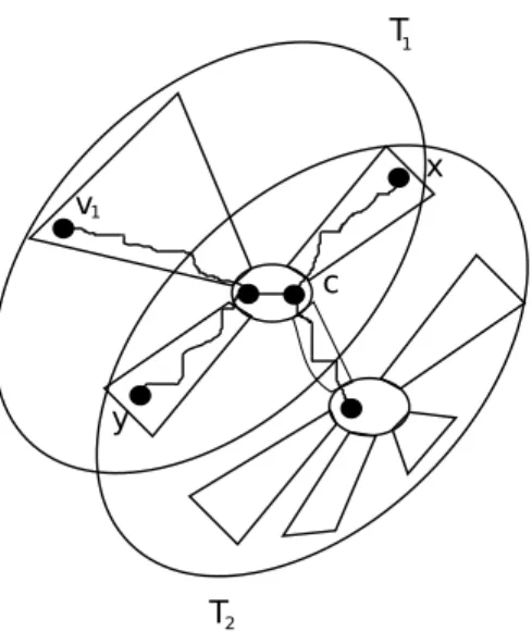
Lemma 3.2. Given a tree T let T1, T2 be two subtrees such that diampT1X T2q “ diampT1q. Then,
we have diampT1Y T2q “ diampT2q.
Proof. First we claim that CpT1X T2q “ CpT1q. Indeed, since T1X T2 and T1 are trees with equal
diameter, and we have T1X T2Ď T1, every diametral path for T1X T2 is also a diametral path for
T1. Furthermore, since on every diametral path in a tree, the middle nodes are exactly the center
nodes (Prop. P-3.1.2), we obtain as claimed that CpT1X T2q “ CpT1q.
Then, let x, y P V pT1X T2q be the two ends of a diametral path in the subtree T1X T2. We set
z P tx, yu maximizing distTpz, CpT2qq and we claim that, for every v1 P V pT1q, distTpv1, CpT2qq ď
v c x y 1 T T 1 2
Figure 3: To the proof of Lemma 3.2.
V pT1q is at a distance ď distTpz, CpT2qq`radpT2q from any node in V pT2q. By unimodality (Prop.
P-3.1.1), eccT2pzq “ distTpz, CpT2qq ` radpT2q ď diampT2q, and so, diampT1Y T2q “ diampT2q.
Finally, in order to prove this above claim there are two cases.
• First assume CpT1q Ď CpT2q. We recall that since the unique xy-path in T must contain all
of CpT1q (Prop. P-3.1.2), there can be no component of T zCpT1q that contains both x, y. In
particular, there exists z P tx, yu such that no component of T zCpT1q can both contain z and
intersect CpT2qzCpT1q. Then, distTpz, CpT2qq “ distTpz, CpT1qq. Furthermore by unimodality
(Prop. P-3.1.1) every node v1P V pT1q has eccentricity distTpv1, CpT1qq ` radpT1q. Since z is
an end in a diametral path of T1 it maximizes distTpz, CpT1qq, and so, for every v1 P V pT1q
we have distTpv1, CpT2qq ď distTpv1, CpT1qq ď distTpz, CpT1qq “ distTpz, CpT2qq.
• Otherwise, let c P CpT1q minimize distTpc, CpT2qq. Note that since we have CpT1q Ę CpT2q,
there is a unique possible choice for c. Furthermore, every v1 P V pT1q satisfies distTpv1, CpT2qq ď
distTpv1, cq ` distTpc, CpT2qq ď radpT1q ` distTpc, CpT2qq, and we will show this upper-bound
is reached for at least one of x or y. Specifically, we can refine one observation from the previous case as follows: there exists z P tx, yu such that no component of T zCpT1q can both
contain z and intersect CpT2qzCpT1q; and in the special case where CpT1q is an edge, c is not
the closest central node to z. In this situation, distTpz, cq “ radpT1q and the path between z
and CpT2q goes by c. See Fig. 3 for an illustration.
In both cases we obtain, as claimed, distTpv1, CpT2qq ď distTpz, CpT2qq for every v1 P V pT1q.
Lemma 3.3. Given a tree T let T1, T2 be two subtrees such that CpT1q Ď CpT2q. Then, we have
that diampT1Y T2q “ maxtdiampT1q, diampT2qu.
Proof. Since CpT1q Ď CpT2q we have for every v1 P V pT1q:
By the unimodality property (Property P-3.1.1) we have that distTpv1, CpT1qq “ eccT1pv1q ´
radpT1q ď diampT1q ´ radpT1q, and so by Property P-3.1.4:
distTpv1, CpT1qq ď tdiampT1q{2u ď maxttdiampT1q{2u , tdiampT2q{2uu.
In the same way, Property P-3.1.4 implies that:
maxtradpT1q, radpT2qu “ maxtrdiampT1q{2s , rdiampT2q{2su.
We so obtain that eccT1YT2pv1q ď maxtdiampT1q, diampT2qu.
Then, for every v2 P V pT2q:
eccT1YT2pv2q ď distTpv2, CpT2qq ` maxtradpT2q, diampCpT2qq ` radpT1qu
ď distTpv2, CpT2qq ` maxtradpT2q, 1 ` radpT1qu.
We may assume radpT1q ě radpT2q since otherwise, eccT1YT2pv2q ď distTpv2, CpT2qq ` radpT2q “
eccT2pv2q ď diampT2q by unimodality (Property P-3.1.1). In particular we claim that it implies
diampT1q ě diampT2q. Indeed, by Property P-3.1.4 we must have rdiampT1q{2s ě rdiampT2q{2s,
and so diampT1q ě diampT2q ´ 1. Moreover since by the hypothesis we also have CpT1q Ď CpT2q, by
Property P-3.1.3 we obtain as claimed diampT1q ě diampT2q (otherwise, diampT1q and diampT2q
must be even and odd, respectively, and so we cannot have rdiampT1q{2s ě rdiampT2q{2s, a
con-tradiction). There are now two cases to consider:
• Case diampT1q “ diampT2q. Then, CpT1q “ CpT2q and we can strengthen our previous
inequality as follows: eccT1YT2pv2q ď distTpv2, CpT2qq ` maxtradpT2q, radpT1qu ď diampT2q.
• Case diampT1q ą diampT2q. Recall that distTpv2, CpT2qq ď tdiampT2q{2u. In particular,
either diampT1q ě diampT2q ` 2, and so, distTpv2, CpT2qq ď tdiampT1q{2u ´ 1; or diampT1q “
diampT2q ` 1 but then, since by the hypothesis we have CpT1q Ď CpT2q, by Property P-3.1.3
diampT1q must be even, and so, distTpv2, CpT2qq ď tdiampT1q{2u ´ 1 also in this case. Overall:
eccT1YT2pv2q ď distTpv2, CpT2qq ` maxtradpT2q, diampCpT2qq ` radpT1qu
ď tdiampT1q{2u ´ 1 ` radpT1q ` 1 “ diampT1q.
Therefore, in both cases we obtain diampT1Y T2q ď maxtdiampT1q, diampT2qu.
3.2 A structure theorem
We are now ready to state the main result in this section:
Theorem 3.4. Given G “ pV, Eq and T any k-Steiner root of G, the following properties hold for any clique-intersection X P X pGq:
• (P-3.4.1.) We have RealpTxXyq “ X and diampTxXyq ď k;
• (P-3.4.2.) If T1
X Ą TxXy then, either X “ RealpTX1 q or diampTX1 q ą diampTxXyq;
• (P-3.4.3.) If C pTxXyq Ď C pTxX1
Proof. We prove each property separately.
(Proof of Property P-3.4.1.) First assume X P K pGq to be a maximal clique. Since all leaves of TxXy are in X, diampTxXyq “ maxu,vPXdistTpu, vq. By the hypothesis T is a
k-Steiner root of G, and so, since X is a clique of G, maxu,vPXdistTpu, vq ď k. In particular,
diampTxXyq ď k, that implies in turn the vertices of RealpTxXyq must induce a clique of G. We can conclude that RealpTxXyq “ X by maximality of X. More generally, let X “ Ş`i“1Ki, for
some family K1, K2, . . . , K` P K pGq. Clearly, TxXy Ď
Ş`
i“1TxKiy, and so, X Ď RealpTxXyq Ď
Ş`
i“1RealpTxKiyq. As we proved before, RealpTxKiyq “ Ki for every 1 ď i ď `, and so,
RealpTxXyq ĎŞ`
i“1Ki“ X. Altogether combined, we obtain that RealpTxXyq “ X.
(Proof of Property P-3.4.2.) Let T1
X Ą TxXy be such that diampTX1 q “ diampTxXyq. We
claim RealpT1
Xq “ X, that will prove the second part of the theorem. Indeed, for any maximal
clique Kj that contains X, we have diampTxKjy X TX1 q ě diampTxXyq “ diampTX1 q, and so,
diampTxKjy Y TX1 q “ diampTxKjyq ď k by Lemma 3.2. It implies RealpTX1 q Ď Kj. Furthermore,
since X P X pGq, X is exactly the intersection of all the maximal cliques Kj that contains it,
thereby proving the claim.
(Proof of Property P-3.4.3.) Finally, assume C pTxXyq Ď C pTxX1yq. By Lemma 3.3 we obtain
that diampTxXy Y TxX1
yq “ maxtdiampTxXyq, diampTxX1yqu ď k. In particular, X Y X1 must be a clique of G.
Before ending this section, we slightly strenghten Property P-3.4.3 of Theorem 3.4, as follows: Lemma 3.5. Given G “ pV, Eq and T any 2k-Steiner root of G, we have C pTxKiyqXC pTxKjyq “ H
for any two different maximal cliques Ki, Kj P K pGq.
Proof. Suppose for the sake of contradiction C pTxKiyq X C pTxKjyq ‰ H, and let r P C pTxKiyq X
C pTxKjyq. By Theorem 3.4 (Prop. P-3.4.1), maxtdiampTxKiyq, diampTxKjyq ď 2k. Thus, any
vertex of TxKiy Y TxKjy is at a distance ď k from r in T (this follows from Prop. P-3.1.4 of
Lemma 3.1). In particular, diampTxKiy Y TxKjyq ď 2k, and so, KiY Kj is a clique of G. The
latter contradicts the fact that Ki, Kj are maximal cliques.
4
Well-structured 4-Steiner roots
We refine our results in the previous Section when k “ 4. Let us start motivating our approach. Given G “ pV, Eq we recall that one of our intermediate goals is to compute, by dynamic program-ming on a clique-tree, subsets Ti of 4-Steiner roots for some collection of subgraphs Gi, with the
following additional property: assuming G is a 4-Steiner power, there must be a partial solution in Ti which can be extended to a 4-Steiner root for G (cf. Sec. 2.3, Step S.3). Ideally, one should store
all the possible 4-Steiner roots for Gi, however this leads to a combinatorial explosion. In order to
(partly) overcome this issue, we introduce the following important notion:
Definition 4.1. Given G “ pV, Eq and X P X pGq, a vertex v P X is called X-constrained if it satisfies one of the following two conditions:
1. either there is another clique-intersection X1
Ă X such that v P X1 and |X1
| ě 2 (we call v internally X-constrained);
2. or there exist X1, X2 P X pGq such that X Ă X1 and X X X2 “ tvu Ă X1 X X2 (we call v
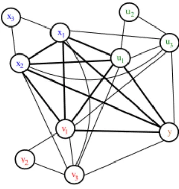
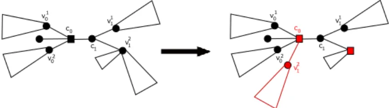
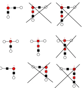
A vertex v P X that is not X-constrained is called X-free. v v v 1 2 3 u u u 1 2 3 x x x 1 2 3 y
Figure 4: Five maximal cliques K1 “ tx1, x2, x3u, K2 “ tu1, u2, u3u, K3 “ tv1, v2, v3u, K4 “
ty, x1, x2, u1, v1, u3u and K5 “ ty, x1, x2, u1, v1, v3u. In the clique-intersection X “ ty, x1, x2, u1, v1u
both vertices x1, x2 are internally X-constrained (for X1 “ X X K1), vertex u1 is pX, K4, K2
q-sandwiched, vertex v1 is pX, K5, K3q-sandwiched and vertex y is X-free.
We refer to Fig. 4 for an illustration of all possibilities. Our study reveals on the one hand that X-constrained vertices have a very rigid structure. It seems on the other hand that X-free vertices are completely unstructured and mostly responsible for the combinatorial explosion of possibilities for TxXy. As our main contribution in this section we prove that we can always force the X-free vertices to be leaves of this subtree TxXy, thereby considerably reducing the number of possibilities for the latter. Specifically:
Theorem 4.1. Let G “ pV, Eq be a 4-Steiner power. There always exists a 4-Steiner root T of G where, for any clique-intersection X P X pGq:
• (P-4.1.1.) all the X-free vertices are leaves of TxXy with maximum eccentricity diampTxXyq; • (P-4.1.2.) there is a node c P C pTxXyq such that for every X-free vertex v, except maybe one,
distTpv, cq “ distTpv, C pTxXyqq;
• (P-4.1.3.) all the internal nodes on a path between C pTxXyq and a X-free vertex are Steiner nodes of degree two;
• (P-4.1.4.) and if X P K pGq and it has a X-free vertex then, diampTxXyq “ 4.
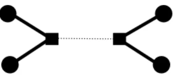
Theorem 4.1 is proved by carefully applying a set of operations on an arbitrary 4-Steiner root until it satisfies all of the desired properties. We give two examples of such operations in Fig. 6 and 7 (see the proof of Theorem 4.1 in order to better understand these two examples). It is crucial for the proof that in any 4-Steiner root of G all the minimal separators yield subtrees of diameter at most three.
In the remaining of the paper, we call a 4-Steiner root with the above properties well-structured. It will appear in Sec. 6, 7, and 8 that we only add partial solutions in the subsets Ti which are in
some sense “close” to the subset of well-structured partial solutions. We first prove Theorem 4.1 for maximal cliques (Section 4.1). This first part of the proof looks easier to generalize to larger values of k. Then, we prove the result in its full generality in Section 4.2.
4.1 The case of (Almost) Simplicial vertices
Let Ki P K pGq be fixed. We start giving a simple characterization of Ki-free vertices in terms of
simplicial vertices and cut-vertices. Then, we prove Theorem 4.1 in the special case when X is a maximal clique.
Lemma 4.2. Given G “ pV, Eq and Ki P K pGq, a vertex v P Ki is Ki-free if and only if:
• either it is simplicial;
• or it is a cut-vertex, and there is no other minimal separator of G contained into Ki that can
also contain v.
Proof. By maximality of Ki, a vertex v P Kican only be either Ki-free or internally Ki-constrained.
In particular, v is Ki-free if and only if for any other Kj P K pGq we have either v R Kj or
KiX Kj “ tvu. As an extremal case, a vertex v P Ki is Ki-free if is not contained into any other
maximal clique, and that is the case if and only if v is simplicial. Thus, from now on assume v is not simplicial. If v P Ki X Kj then, in any clique-tree TG of G, the vertex v and more generally,
all of KiX Kj, is contained into all the minimal separators that label an edge of the KiKj-path
in TG. This implies that there is always a largest clique-intersection X Ă Ki containing v that is
a minimal separator. Hence a non simplicial v P Ki is Ki-free if and only if it is a cut-vertex and
there is no other minimal separator in Ki that contains this vertex.
Lemma 4.3. Let G “ pV, Eq be a 4-Steiner power. There exists a 4-Steiner root T of G such that the following hold for any maximal clique Ki:
• If there is at least one Ki-free vertex then, diampTxKiyq “ 4;
• every Ki-free vertex v is a leaf of TxKiy. Moreover distTpv, C pTxKiyqq “ 2 and the internal
node onto the unique vC pTxKiyq-path is a degree-two Steiner node.
Proof. We give an illustration of the proof in Fig. 5. First we pick an arbitrary 4-Steiner root T of G, that exists by the hypothesis. Define S1 to be the set of all the cut-vertices in G that are
Ki-free for some KiP K pGq. We now proceed by induction on |S1|.
Assume S1 “ H for the base case. For every maximal clique Ki, by Lemma 4.2, the Ki-free
vertices are exactly the simplicial vertices in Ki. We consider all the simplicial vertices v P Ki
sequentially, and we proceed as follows. Let ci P C pTxKiyq minimize distTpv, ciq (possibly, v “ ci).
We first replace v by a Steiner node α. In doing so, we get a 4-Steiner root T1 for Gzv. Then,
let c1
i be either ci (if ci ‰ v) or α (if ci “ v). We connect v to c1i via a path of length exactly
4 ´ maxuPKiztvudistT1pc1i, uq of which all internal nodes are Steiner. In doing so, we obtain a tree
T2 such that RealpT2
q “ V . By construction, maxuPKiztvudistT1pc
1
i, uq ď eccTxKiypciq ď 2 (since
diampTxKiyq ď 4). It implies:
distTpv, ciq ď eccTxKiypciq ď 4 ´ max
uPKiztvu
distT1pc1i, uq “ distT2pv, c1iq.
As a result, the distances between real nodes can only increase compared to T, and this new tree T2 we get keeps the property of being a 4-Steiner root of G. Furthermore, diampT2
xKiyq “ 4 and
the unique central node in C pT2
0
1
2
3
4
5
6
7
0
1
2
3
4
5
6
7
0
1
2
3
3
4
5
6
7
0
1
2
3
4
5
6
7
0
1
2
4
5
6
7
3
4
and v cannot falsify the properties of the lemma at any further loop. Overall, after this first phase is done we may assume that all the simplicial vertices v are contained into some maximal clique Ki such that: diampTxKiyq “ 4, v is a leaf of TxKiy such that distTpv, C pTxKiyqq “ 2, and the
internal node onto the vC pTxKiyq-path is Steiner.
From now on we assume S1‰ H. Let v P S1and let C1, C2, . . . , C`be the connected components
of Gzv. For every i P t1, 2, . . . , `u, the graph Gi :“ GrCi Y tvus is a 4-Steiner power as this is a
hereditary property. Specifically, given a fixed 4-Steiner root T for G, we obtain a 4-Steiner root Tpiq for G
i by replacing every vertex in V pGqzV pGiq by a Steiner node. By induction, we can
modify all the subtrees Tpiq into some new subtrees Tpi,2q that satisfy the properties of the lemma
w.r.t. Gi. Overall, by identifying all the Tpi,2q’s at v, one obtains a tree T1. We claim that T1
satisfies the two properties of the lemma. Indeed, it follows from the characterization of Lemma 4.2 that, for any maximal clique Kj Ď CiY tvu, the Kj-free vertices in G are still Kj-free vertices in
Gi. – Note that in particular, if v is Kj-free in G then, v is simplicial in Gi. – Therefore, the
claim is proved. It remains now to show that T1 is indeed a 4-Steiner root of G. This is not the
case only if there exist x P Cp, y P Cq such that p ‰ q and distT1px, vq ` distT1pv, yq ď 4. Our
construction implies distT1px, vq ě distTpx, vq and distT1py, vq ě distTpy, vq. But then, we should
already have distTpx, yq ď 4 in the original root T. Thus, since T is a 4-Steiner root of G, this case
cannot happen and T1 is also a 4-Steiner root of the graph G.
4.2 The general case
We are now ready to prove Theorem 4.1 in its full generality:
Proof of Theorem 4.1. Let T be such that the result holds for maximal cliques (such a T exists by Lemma 4.3). For any X P X pGq zK pGq with at most two elements, the properties of the theorem always hold (for any T). We so only consider the clique-intersections X P X pGq zK pGq with at least three elements. Then, diampTxXyq ď 3 by Theorem 3.4 – Prop P-3.4.2 (i.e., because X is strictly contained into some maximal clique K and so, diampTxXyq ă diampTxKyq). In what follows, we will often use properties of the subtree TxXy that only hold if diampTxXyq ď 3; namely:
• TxXyzC pTxXyq is a collection of leaf-nodes;
• there are at least two leaf-nodes (i.e., because |X| ě 3), and there is at least one leaf-node adjacent to every central node in C pTxXyq;
• (as a direct consequence of the previous property) every central node in C pTxXyq has at least two neighbours in TxXy.
In particular, Property P-4.1.3 is now implied by Property P-4.1.1 as there can be no internal node on the path between a leaf and the closest central node. In the same way, Property P-4.1.1 can be slightly simplified as every leaf has maximum eccentricity; hence, we only need to ensure that X-free vertices are leaves. Finally, this also implies that SteinerpTxXyq Ď C pTxXyq, as all leaves of TxXy must be in X(i.e., by the very definition of TxXy).
The proof follows from different uses of a special operation on the tree T that we now introduce: Operation 1. Let X P X pGq zK pGq have size at least three and let v P X. We define Rv to be
the forest of all the subtrees in TzTxXy that contain one node adjacent to v and have no real node at a distance ď 4 from Xztvu in T. Let Qv be the subtree of T that is induced by RvY tvu.
1. We remove Rv and we replace v by a Steiner node αv. In doing so, we obtain an intermediate
tree denoted by Tv. Note that Tv contains the subtree TvX: that is obtained from TxXy by
replacing v with αv (and so, is isomorphic to TxXy);
2. In order to obtain T1 from T
v, we add a copy of Qv and an edge vc between v and a center
node of TvX (possibly, c “ αv).
We refer to Fig. 6 and 7 for some particular applications of Operation 1. Furthermore in what follows we prove that under some conditions of use, this above Operation 1 always outputs a 4-Steiner root T1 that is closer to satisfy all the properties of the theorem than T. Specifically:
Claim 4.3.1. Assume that v is X-free and that every center node of TxXy is adjacent to a real node in Xztvu. Then, T1 keeps the property of being a 4-Steiner root of G if and only if the following
conditions hold:
• (Condition 4.3.1.a) either distTpRealpRvq, vq ě 4 or c is Steiner;
• (Condition 4.3.1.b) if c ‰ αv then, distTvpc, V zNGrvsq ą 3.
Moreover, for any X1
P X pGq ztXu, if any of Properties P-4.1.1, P-4.1.2, P-4.1.3 or P-4.1.4 is satisfied for X1 in T then, this stays so in T1.
Proof. First we prove that all the real vertices in Rv are at a distance ą 4 from V pGqzV pQvq in
the original tree T (Subclaim 4.3.1.1). This will help us in better understanding the structure of T in the remaining of the proof.
Subclaim 4.3.1.1. distTpRealpRvq, V pGqzV pQvqq ą 4.
Proof. Suppose for the sake of contradiction that there exist x P RealpRvq, y R V pQvq such that
distTpx, yq ď 4. Then, v is onto the unique xy-path in T. Furthermore, recall that by definition
of Rv, distTpx, Xztvuq ą 4. By the hypothesis every central node of C pTxXyq is adjacent to a
vertex of Xzv, and so we have distTpv, Xztvuq ď 2. As a result, we obtain distTpv, xq “ 3 and
distTpv, yq “ 1. But then, y is at a distance ď diampTxXyq ` 1 ď 4 from any vertex in X, that
implies the existence of a clique-intersection X1 Ě X Y tyu. Let X2 be any clique-intersection
that contains all of x, y, v. Since we assume distTpx, Xztvuq ą 4, X X X2 “ tvu and in particular,
X1‰ X2. It implies that v is pX, X1, X2q-sandwiched, a contradiction. ˝
It follows from Subclaim 4.3.1.1 that in order for T1 to be a 4-Steiner root for G, one must
ensure distT1pRealpRvq, V zV pQvqq ą 4. We then prove that this above condition is
equiva-lent to Condition 4.3.1.a. Indeed, note that we always have distT1pRealpRvq, V zV pQvqq ą 4 if
distTpv, RealpRvqq ě 4. Otherwise, by the hypothesis every center node of C pTxXyq is adjacent
to a real node in Xztvu, thereby implying distTpv, V zV pQvqq ď distTpv, Xztvuq ď 2, and so,
distTpv, RealpRvqq “ 3. Then, a necessary and sufficient condition for having that
distT1pRealpRvq, V zV pQvqq ą 4 is that c is Steiner.
In the same way, Condition 4.3.1.b implies the necessary condition distT1pu, vq ą 4 for every
u R NGpvq. However, the above does not prove that T1 is a 4-Steiner root of G yet, as we also need
to ensure distT1pu, vq ď 4 for every u P NGpvq. In order to prove this is the case, and to also prove
the second part of the claim, we now consider the clique-intersections X1
P X pGq ztXu such that v P X1. (Note that if v R X1 then, TxX1y “ T1xX1y and so, the result of our claim trivially holds for
such a X1). Since we have dist
TpRealpRvq, V zV pQvqq ą 4 (Subclaim 4.3.1.1), there are only two
possibilities: either TxX1y is fully contained into Q
v – in which case it is not modified –; or it does
not intersect Rv. We then consider two different cases:
• Assume X Ă X1. In particular, TxX1
y X Rv “ H. It implies that T1xX1y is obtained from
TxX1y by replacing v by a Steiner node (only if it were an internal node of TxX1y) then,
making of v a leaf.
Subclaim 4.3.1.2. diampT1
xX1yq “ diampTxX1yq. Proof. We divide the proof into two parts:
– In order to prove diampT1
xX1yq ď diampTxX1yq, we consider an auxiliary subtree T2xX1y: obtained from the original TxX1
y by adding a leaf v1 to some arbitrary central node c1
in C pTxXyq. Note that T1xX1y is isomorphic to a subtree of T2xX1y for the choice of
c1
“ c. Furthermore since c1 has at least two neighbours in TxXy Ď TxX1
y we have: diam`TxX1y X pNTxX1yrc1s Y tv1uq
˘
“ diampNTxX1yrc1sq “ 2 “ diampNTxX1yrc1s Y tv1uq.
We so deduce from Lemma 3.2 that:
diampT2xX1yq “ diampTxX1y Y pNTxX1yrc1s Y tv1uqq “ diampTxX1yq.
In particular, diampT1
xX1yq ď diampT2xX1yq “ diampTxX1yq. – For the converse direction, it suffices to prove, if TxX1
y ‰ T1xX1y, the existence of a diametral path in TxX1
y of which v is not an end. Since the ends of a diametral path must be leaves, we can restrict our study to the case where: v is a leaf of TxXy, and there is no subtree of TxX1yzTxXy that contains a neighbour of v in T. In particular, TxXy ‰ T1xXy
(otherwise TxX1
y “ T1xX1y, and so we are done). We deduce from the above that v is adjacent to a central node c1 P C pTxXyq, and c1 ‰ c (otherwise TxXy “ T1xXy,
a contradiction). Then, C pTxXyq “ tc, c1u and so, TxXy is a bistar (diameter-three
subtree). Recall that both c, c1have a neighbour in Xztvu by the hypothesis. This implies
that node c1 must have at least two neighbours in TX
v ; moreover each such neighbour
must be on the path between c1 and a real node in Xztvu. But then, since there are
at least three branches in TxX1
yztc1u, we obtain as desired the existence of a diametral path in TxX1
y of which v is not an end. As a result, diampT1xX1yq ě diampTxX1yq. Altogether combined, the above proves the subclaim that diampT1xX1yq “ diampTxX1yq. ˝
By Subclaim 4.3.1.2, we cannot change diampTxX1
yq and so, it immediately implies that we cannot break Property P-4.1.4. The proof of this subclaim is actually more precise as it also shows that if T1xX1y ‰ TxX1y then, these two subtrees have a common diametral pair px, yq,
for some x, y ‰ v. In particular (Prop. P-3.1.2 of Lemma 3.1), we also have that: C`T1 xX1y˘“ # C pT xX1 yq if v R C pT xX1yq pC pT xX1yq ztvuq Y tαvu otherwise.
Furthermore, for any u P X1
ztvu, if Pudenotes the uC pTxX1yq-path in T then, the uC pT1xX1
yq-path in T1 can be obtained from P
u by replacing v with αv. – This above analysis
above mapping implies that we cannot break Properties P-4.1.2 and P-4.1.3. It also im-plies distT1pu, C pT1xX1yqq “ distTpu, C pTxX1yqq and so, by unimodality (Prop. P-3.1.1 of
Lemma 3.1) we did not change the eccentricity of any vertex u P X1
ztvu. Altogether com-bined, every X1-free vertex that was a leaf of TxX1
y is also a leaf of T1xX1y with same eccentricity (Property P-4.1.1 cannot be broken).
Finally, we also obtain distT1pu, vq ď 4 for every u P X1 (i.e., T1 is a 4-Steiner root of G).
• Otherwise, X Ę X1 and we prove TxX1
y “ T1xX1y. To see that, suppose for the sake of contradiction TxX1y ‰ T1xX1y. We first note this may be the case only if TxX1y is not fully
contained into Qv.
Subclaim 4.3.1.3. TxX1y must intersect TxXyztvu.
Proof. Suppose by contradiction that TxX1
y X TxXy “ tvu. As we also assume TxX1y is not fully contained into Qv, we have TxX1y X Rv “ H. Then, TxX1y must intersect some subtree
Tpsubq of TzTxXy that is not in R
v. Let x P X1X Tpsubq. By the definition of Rv, there must
exist x1
P RealpTpsubqq such that: distTpx1, Xztvuq ď 4 (possibly, x “ x1). In particular,
note that there exists a xx1-path that does not go by v in T (otherwise, x, x1 would be in
different subtrees of TzTxXy). On one hand as we assume v to be X-free, there must exist a clique-intersection X1 Ě X Y tx1u. It implies distTpx1, vq ď 2 because eccTxXypvq ě 2. On
the other hand, we also know that distTpx, vq ď 4. By considering the median node of the
triple x, x1, v we so obtain dist
Tpx, x1q ď 4. Let X2 be a clique-intersection that contains all
of x, x1, v (possibly, X
2 “ X1). There are two cases:
– If X Ę X2 then, X X X2 “ tvu (otherwise, v would be internally X-constrained). But
in this case, v is pX, X1, X2q-sandwiched, a contradiction.
– Otherwise, X Ď X2. However by the hypothesis X Ę X1, and so X X X1 “ tvu
(otherwise, v would be internally X-constrained). It implies v is pX, X2, X1q-sandwiched,
a contradiction. As a result, TxX1
y must intersect TxXyztvu. ˛
Finally, since v is X-free any node β P V pTxX1
yqXpV pTxXyqztvuq must be Steiner. This leaves β P C pTxX1
yq ztvu as the only possibility. Furthermore, since β is Steiner there must exist y P X1such that the unique vy-path in T goes by β. However, this implies diampTxX1YN
Trβsyq “
diampTxX1
yq. We recall that there exists at least one leaf node u P RealpNTpβqqztvu by the
hypothesis. Thus, by Property P-3.4.2 of Theorem 3.4 we have u, v P X X X1, thereby
contradicting that v is X-free.
The claim directly follows from this above case analysis. ˛
The proof is now divided into two main phases.
Phase 1: Transformation into leaves (see Fig. 6 for an illustration). Let X P X pGq zK pGq , |X| ě 3 be fixed. We first transform T so that all the X-free vertices are leaves in TxXy. Assume the existence of a X-free vertex v P X that is not a leaf. Note that we have v P C pTxXyq because
v
Qv
v
Qv
B B
Figure 6: Forcing the X-free vertices as leaves.
diampTxXyq ď 3. In particular, every node in C pTxXyq is adjacent to a leaf in Xztvu. We apply Operation 1 with c “ αv (i.e., the Steiner node substituting v in the intermediate tree Tv). Since
c “ αv and so, in particular c is Steiner, both Conditions 4.3.1.a and 4.3.1.b of Claim 4.3.1 must
hold. Overall, by Claim 4.3.1 we can repeat the above transformation until all the X-free vertices are leaves of TxXy.
c c v v v v 0 0 0 1 1 1 1 1 2 2 c c v v v v 0 0 0 1 1 1 1 1 2 2
Figure 7: Grouping the X-free vertices on a same side.
Phase 2: Grouping the X-free vertices (see Fig. 7 for an illustration). After Phase 1, the properties of the theorem are true for any X P X pGq such that TxXy is a star. Thus, from now on assume TxXy is a bistar (diameter-three subtree). Write C pTxXyq “ tc0, c1u and assume that
each cj is adjacent to two X-free vertices, denoted vj1, vj2. For any i P t1, 2u, there is no vertex
xi P RealpRvi
jq such that distTpxi, v
i
jq ď 2 (otherwise, distTpxi, Xztvijuq ď distTpxi, v3´ij q ď 4,
a contradiction). More specifically, either distTpvij, RealpRvi
jqq ě 4, or distTpv
i
j, RealpRvi jqq “ 3
but then cj must be Steiner (otherwise, distTpxi, Xztvjiuq ď distTpxi, cjq ď 4, a contradiction).
Furthermore, we can have distTpu, cjq ď 3 only if X Ď NGrus (i.e., because cj is adjacent in T to
at least two X-free vertices).
W.l.o.g., assume either distTpvji, RealpRvi
jqq ě 4 for any i, j or c0 is Steiner. If in addition both
c0, c1 are Steiner nodes (real nodes, resp.) then, we further assume w.l.o.g. c0 is adjacent to more
X-free vertices than c1. We apply Operation 1 for v “ v11 and c “ c0. Note that by construction,
c0 always satisfies Condition 4.3.1.a of Claim 4.3.1. Since we also have distTpu, c0q ď 3 ùñ X Ď
NGrus, Condition 4.3.1.b of Claim 4.3.1 is satisfied. Overall, we can repeat this transformation
until X satisfies all the properties stated in the theorem, that does not impact the properties of the other clique-intersections X1 by Claim 4.3.1.
5
Step S.1: Construction of the clique-tree
Our main result in this section is that every chordal graph has a polynomial-time computable rooted clique-tree where some technical conditions must hold on the minimal separators that can
label an edge (Theorem 5.4). We will use these special properties of our rooted clique-tree in order to ensure that our main algorithm runs in polynomial time.
We start digressing on the motivations behind our construction. Given a rooted clique-tree TG of G and an arbitrary maximal clique Ki, recall that Gi is the subgraph induced by all the
maximal cliques in the subtree TGi rooted at Ki. Assume that TxSiy: the subtree induced by the
minimal separator Si :“ KiX Kppiq, is fixed. We ask for the number of possible distance profiles
pdistTipr, VizSiqqrPV pTxSiyq over all possible well-structured 4-Steiner roots of Gi that contain TxSiy.
By Theorem 4.1, one way to bound this number would be to force most vertices in Si to be Ki-free
in the subgraph Gi. Guided by this intuition, our construction aims at preventing Si to contain,
or to be contained, in a minimal separator of Gi. Since both objectives are conflicting, this results
in a technical compromise.
We present a first, simpler construction in Section 5.1 that only reaches half of the goal. Then, we introduce the new notion of (weak) convergence, and we show its relationship with 4-Steiner powers (Section 5.2). We end up proving the main result of this part in Section 5.3.
5.1 A flat clique-tree
We start with an intermediate construction.
Theorem 5.1. Given G “ pV, Eq chordal, we can compute in polynomial time a rooted clique-tree TG such that, for any Si “ KiX Kppiq and for any child Kj of Kppiq, there is no minimal separator
of Gj that is contained into Si.
Proof. We modify an arbitrary clique-tree TG of G until the property of the theorem is satisfied.
Specifically, root TGat some arbitrary maximal clique K0. We consider all the minimal separators
S P S pGq by decreasing size. Let KS be incident to an edge in
Ť
S1,SĎS1ES1pTGq and the closest
possible to the root. We observe that KS is the least common ancestor of all maximal cliques that
are incident to an edge inŤ
S1,SĎS1ES1pTGq. Furthermore all edges in ESpTGq can be made incident
to KS, as follows. Assume there exists KiKppiqP ESpTGq such that KS R tKi, Kppiqu. By the above
observation, Ki, Kppiq are into the subtree rooted at KS. Since S Ď KSX Ki, S is contained into
all the maximal cliques on the KSKi-path. In particular, we still obtain a clique-tree of G if we
replace KiKppiq by KiKS and in doing so, S Ď KSX KiĎ KppiqX Ki “ S. Furthermore after this
transformation, KS became the new father node of the maximal clique Ki in TG.
It now remains to prove that the gotten clique-tree TG satisfies the conditions of the theorem.
Suppose for the sake of contradiction that there exist i ą 0 and Sk Ď Si a minimal separator
of Gj, where Kj is a child of Kppiq (possibly, i “ j). We observe that after we processed Si, all
edges in ESipTGq must label an edge between KSi “ Kppiq and its children nodes. Therefore, our
transformation ensures Sk‰ Si, i.e., SkĂ Si. Since the subtree rooted at Kj is a rooted clique-tree
of Gj, there must exist some edge KkKppkq in this subtree such that KkX Kppkq “ Sk. However,
since we consider minimal separators by increasing size, the edge KiKppiqshould already exist when
we process Sk. It implies that the maximal clique KSk to which we connected all edges in ESkpTGq
should be an ancestor of Kppiq, that is a contradiction.
5.2 Weak convergence
Unfortunately, the “flat” clique-tree of Theorem 5.1 does not prevent the case when a minimal sep-arator Si is contained into a minimal separator of Gi. As a new step toward our final construction,
we now introduce the following notions:
Definition 5.1. Given a clique-tree TG of G “ pV, Eq, we say that a minimal separator S is
weakly TG-convergent if there exists some maximal clique KS that is incident to all edges in
Ť
S1,SĂS1ES1pTGq. S is termed TG-convergent if it is weakly TG-convergent and the maximal clique
KS is also incident to all edges in ESpTGq.
In order to motivate Definition 5.1, in what follows are two observations on the relationships between clique-trees, minimal separators and 4-Steiner roots:
Lemma 5.2. Given G “ pV, Eq and T any 4-Steiner root of G, let Ki P K pGq and let X Ă Ki be
a clique-intersection. If TxXy is a bistar then, C pTxKiyq Ă C pTxXyq.
In particular, there are exactly two maximal cliques that contain X.
Proof. We have by Theorem 3.4 diampTxKiyq ą diampTxXyq, and so, diampTxKiyq “ 4. In
particular, write C pTxKiyq “ tciu. Every component in TxKiyztciu has diameter at most two,
thereby implying ci P V pTxXyq. Furthermore since eccTxXypciq ď radpTxKiyq “ 2, ci cannot be a
leaf of TxXy. Equivalently, ci P C pTxXyq. By Lemma 3.5, there can be no two maximal cliques
Ki, Kj P K pGq such that C pTxKiyq “ C pTxKjyq. Therefore, the above implies that X can only be
contained in at most two maximal cliques. Finally, since X is not a maximal clique, it is contained into exactly two maximal cliques.
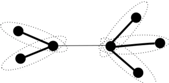
Lemma 5.3. Given G “ pV, Eq and T any 4-Steiner root of G, let S P S pGq. If TxSy is a non-edge star then, S is weakly TG-convergent for any clique-tree TG of G.
Proof. We may assume that S is strictly contained into at least one minimal separator S1 for
otherwise there is nothing to prove. By Theorem 3.4, TxS1y is a bistar and S1 must be inclusion
wise maximal in S pGq. This implies C pTxSyq Ă C pTxS1yq. Furthermore, it follows from Lemma 5.2
that S1 must be contained into exactly two maximal cliques K
i, Kj and C pTxKiyq Y C pTxKjyq “
C pTxS1
yq. In particular, we may assume w.l.o.g. that C pTxSyq “ C pTxKiyq. But then, still by
Lemma 5.2, any minimal separator S2 that strictly contains S must be contained into K i and
exactly one other maximal clique KS2. By Theorem 2.4, the latter implies KiKS2 P EpTGq and
KiX KS2 “ S2.
Roughly, in order to prove Theorem 5.4 we will slightly modify the construction of Theorem 5.1 so as to force weak convergence to imply convergence. In doing so we will obtain that for a fixed minimal separator S, we may encounter some “inclusion issue” between S and another minimal separator S’ at most once. We will show in Sec. 7 that this above “local” property of our clique-tree is enough in order to bound the number of possible distance profiles at each node of the clique-tree by a polynomial.
5.3 The final construction
The remaining of this section is now devoted to prove the following technical result:
Theorem 5.4. Given G “ pV, Eq chordal, we can compute in polynomial time a rooted clique-tree TG where the following conditions are true for any Si :“ KiX Kppiq, i ą 0:
• (Prop. P-5.4.2.) Any minimal separator of Gi that is contained into Si is TG-convergent, it
has at least three vertices and it is strictly contained into at least one minimal separator of Gi.
We stress that in the above two statements, 3 can be replaced by any positive integer q. However, please note that such a change would affect both properties of the theorem.
Proof. We start describing the algorithm before proving its correctness. In what follows, the mini-mal separators of G are considered in the same order for every phase of the algorithm.
Phase 1 Let TGbe an arbitrary unrooted clique-tree. We consider all the minimal separators S P S pGq
by decreasing size. Let S1, S2, . . . , Spbe the list of all minimal separators containing S ordered by decreasing size. – In particular, Sp “ S, and if several such minimal separators Si have equal size then, we break ties according to the ordering in which they are considered. – For every maximal clique K, we can define a binary vector ÝÑvSpKq “ pδSK1, δSK2, . . . , δSKpq: where
δSKi “ 1 if and only if K is incident to an edge in ESipTGq. Then, we choose KS1 P K pGq such
that ÝvÑSpKS1q is lexicographically maximal. While there exists an edge KK1 P ESpTGq such
that KS1 R tK, K1u, we do as follows. W.l.o.g., K is on the KS1K1-path. We replace the edge
KK1 by K1
SK1. Doing so, all edges in ESpTGq are now incident to KS1.
Phase 2 We root TG at some arbitrary maximal clique K0. Then, we consider all the minimal
sepa-rators S P S pGq by decreasing size. Let KS2 be, under the following conditions, the closest possible to the root:
• K2
S is incident to an edge in
Ť
S1,SĎS1ES1pTGq;
• and if |S| ě 3 and S is TG-convergent then, KS2 is incident to all edges in
Ť
S1,SĂS1ES1pTGq.
Note that KS2is always an ancestor of KS1. In particular if |S| ě 3 and S is TG-convergent then,
KS2 is either KS1 or its parent node (with the latter being possible only if |Ť
S1,SĂS1ES1pTGq | ď
1). Then, we use the same operation as in the proof of Theorem 5.1 in order to make all edges in ESpTGq incident to KS2.
Phase 3 We end up considering all the minimal separators S P S pGq by decreasing size. If |S| ě 3 and S is not TG-convergent then, we search for a child KS3 of KS2 that is incident to all edges
inŤS1,SĂS1ES1pTGq. For simplicity of our analysis, we will also set KS3 “ KS2 when |S| ď 2,
or S is already TG-convergent, or there is no child node of KS2 which satisfies the desired
property. Then, we consider all the children K of K2
S, K ‰ KS3, such that K X KS2 “ S. We
replace the edge KKS2 by KKS3.
Before proving correctness of this above algorithm, we want to emphasize two of its main invariants. In what follows, let S P S pGq be of size at least three.
• (Inv. I1) Assume that at the time we considered S during Phase 2, S was TG-convergent. We observe that our choice for KS2 preserved this property. In particular, S is TG-convergent in
the final clique-tree TG that we output.
• (Inv. I2) If K3
S ‰ KS2 (or equivalently, we modify ESpTGq during Phase 3) then, we also claim
that S is TG-convergent in the final clique-tree TGthat we output. For that, by the definition