HAL Id: hal-01236488
https://hal.inria.fr/hal-01236488v2
Submitted on 13 Apr 2016
HAL is a multi-disciplinary open access
archive for the deposit and dissemination of
sci-entific research documents, whether they are
pub-lished or not. The documents may come from
teaching and research institutions in France or
abroad, or from public or private research centers.
L’archive ouverte pluridisciplinaire HAL, est
destinée au dépôt et à la diffusion de documents
scientifiques de niveau recherche, publiés ou non,
émanant des établissements d’enseignement et de
recherche français ou étrangers, des laboratoires
publics ou privés.
Distributed under a Creative Commons Attribution - NonCommercial - NoDerivatives| 4.0
Nonsmooth simulation of dense granular flows with
pressure-dependent yield stress
Gilles Daviet, Florence Bertails-Descoubes
To cite this version:
Gilles Daviet, Florence Bertails-Descoubes.
Nonsmooth simulation of dense granular flows with
pressure-dependent yield stress. Journal of Non-Newtonian Fluid Mechanics, Elsevier, 2016, 234,
pp.15-35. �10.1016/j.jnnfm.2016.04.006�. �hal-01236488v2�
Nonsmooth simulation of dense granular flows
with pressure-dependent yield stress
Gilles Daviet
Florence Bertails-Descoubes
∗April 13, 2016
Abstract
Understanding the flow of granular materials is of utmost importance for numerous industrial applications includ-ing the manufacturinclud-ing, storinclud-ing and transportation of grain assemblies (such as cement, pills, or corn), as well as for natural risk assessing considerations. Discrete Element Modeling (DEM) methods, which explicitly represent grain-grain interactions, allow for highly-tunable and precise simulations, but they suffer from a prohibitive computational cost when attempting to reproduce large scale scenarios. Continuum models have been recently investigated to over-come such scalability issues, but their numerical simulation still poses many challenges. In this work we propose a novel numerical framework for the continuous simulation of dilatable materials with pressure-dependent (Coulomb) yield stress. Relying upon convex optimization tools, we show that such a macroscopic, nonsmooth rheology can be interpreted as the exact analogous of the solid frictional contact problem at the heart of DEM methods, extended to the tensorial space. Combined with a carefully chosen finite-element discretization, this new framework allows us to avoid regularizing the continuum rheology while benefiting from the efficiency of nonsmooth optimization solvers, mainly leveraged by DEM methods so far. Our numerical results successfully compare to analytic solutions on model problems, and we retrieve qualitative flow features commonly observed in reported experiments of the literature.
1
Introduction
1.1
Motivation
Granular media are common both naturally and in indus-trial processes, and understanding their flow is crucial to several applications, such as studying the evolution of the pressure in a silo discharge or predicting the run-out of avalanches. Consequently, the past decades have yielded extensive bodies of research dedicated to the modeling of such materials. However, to this day their numerical simulation remains a challenging problem.
In this work we focus on a continuum model for granular-like materials satisfying two key properties. First, we assume that the material cannot be compacted, while it is allowed to dilate as desired, i.e., the divergence of the velocity field is non-negative everywhere, but not necessarily equal to zero. Second, we consider that the material behaves as a viscoplastic fluid whose yield stress depends linearly on the local pressure. Intuitively, this comes from the assumption that grain-grain interactions mostly involve rigid-body contacts with Coulomb fric-tion.
∗INRIA Grenoble Rhône-Alpes and Laboratoire Jean Kuntz-man, 655 avenue de l’Europe, 38334 Saint- Ismier, France. {gilles.daviet,florence}[email protected]
1.2
Related work
1.2.1 Discrete Elements Modeling
A natural way to model granular materials is to proceed at the grain level.
Stemming from the seminal work of Jean-Jacques Moreau, nonsmooth methods for simulating frictional contacts between discrete bodies have been the sub-ject of extensive research in the last three decades. Alart and Curnier [Alart and Curnier, 1991] proposed one of the first formulation of Coulomb friction that is well-suited for nonsmooth optimization methods. Using an operator-splitting scheme, Jean and col-leagues [Jourdan et al., 1998, Jean, 1999] managed to make it scale to very large number of contacts. Their work became known as the Nonsmooth Contact
Dy-namics (NSCD) method. As it will be of great rele-vance in the technical content of this paper, we also point out the change of variable introduced by De Saxcé and Feng [De Saxcé and Feng, 1998] who refor-mulated the discrete-time contact problem as a (non-linear) Second-Order Cone complementarity problem. Cadoux [Cadoux, 2009] used this point of view to formu-late a criterion for the existence of solutions, as well as an algorithm for finding one solution, relying on a series of Second-Order Cone Quadratic Programs.
Those grain-level methods are still the subject of exten-sive work in the context of granular materials, in regard
of both their computational efficiency [Alart et al., 2012, Kleinert et al., 2014] and their ability to describe specific materials [Lim et al., 2014].
However, since they have to take into account ev-ery contact between grains, the cost of DEM meth-ods increases tremendously when considering scenar-ios where the particles are very small w.r.t. the computational domain. This motivates the need for a continuum description of the material. Some au-thors have also developed hybrid methods which at-tempt to retain the precision of DEM while tackling larger computational domains [Bardenhagen et al., 2000, Wellmann and Wriggers, 2012]. In this case, an efficient way to solve the dynamics of the continuous part of the model is still required.
1.2.2 Continuous modeling of granular materials
In the last decade, the introduction of the µ(I) rhe-ology [Jop et al., 2006, GDR MiDi, 2004] contributed to the growth of a large body of research on continuous mod-els for dry granular materials. In particular, the µ(I) rhe-ology was validated against Discrete Element Modeling simulations on complex scenarios such as the collapse of a granular column [Lagrée et al., 2011] or the discharge of silos [Kamrin, 2010,Staron et al., 2014].
In a very recent work, Ionescu et al.
[Ionescu et al., 2015] were able to reproduce experi-mental collapses of granular columns using either the full µ(I) rheology, or a constant friction coefficient µ and a constant Newtonian viscosity. Here we shall focus on the latter case of a constant µ, though we show in Section 6.2.2 that our method may accommodate more complex rheologies with little modification.
Several works have focused on the simulation of such a model, most of them considering the flow to be incompressible [Lagrée et al., 2011, Chambon et al., 2011, Staron et al., 2014, Ionescu et al., 2015,Chauchat and Médale, 2014]. How-ever, this choice may prove unfortunate in certain config-urations, such as the wake of an obstacle, where special care has to be taken to ensure that the rheology remains well-defined [Chauchat and Médale, 2014]. In contrast, Dunatunga and Kamrin [Dunatunga and Kamrin, 2015] recently used an explicit Material Point Method to model compressible granular flows. In a similar manner, our method does not preclude the expansion of the flow. However, we consider a purely rigid solid regime instead of an elastic one, and focus our analysis on the dense limit. Compared to prior art, the main novelty of our approach is to propose to solve the rheology constraints in an implicit manner, by leveraging tools from nonsmooth optimization. This allows us to capture directly the steady-state of non-inertial flows.
1.2.3 Numerical simulation of yield-stress flows
Yield-stress fluids, especially those exhibiting Bingham or Herschel–Bulkley rheologies, have been widely in-vestigated experimentally and numerically, due to their
numerous industrial applications. Due to the non-differentiability of their rheology, simulating yield-stress fluids using an explicit scheme requires the use of very small time-steps; on the other hand, devising implicit methods pose theoretical difficulties. Such implicit ap-proaches are usually instances of either:
• Regularizing methods, which employ diverse nu-merical artifacts to smooth out the singularities of the rheology (see, e.g., [Frigaard and Nouar, 2005] for a review). The main benefit of a regular-izing strategy is the use of classical numerical schemes dedicated to differential equations. How-ever such methods may lead to stiff equations, mak-ing them unable to capture fully rigid zones prop-erly [Saramito and Roquet, 2001];
• Augmented Lagrangian methods, based on the framework of [Fortin and Glowinski, 1982]. Their main drawback is the slow convergence rate often observed in practice.
Very recently, Bleyer et al. [Bleyer et al., 2015] proposed a method for Herschel–Bulkley fluids based on the non-smooth convex optimization theory, which they claim benefits from much faster convergence properties than Augmented Lagrangian methods. In a similar spirit, our approach builds a nonsmooth model for the class of di-latable and pressure-dependent yield stress flows (such as granular materials), and leverages the efficiency of optimization-based solvers for making the numerical solv-ing tractable.
1.3
Contributions
More specifically, our contributions include:
• A viscoplastic rheology for dense granular flows with a Drucker-Prager yielding criterion and an unilateral incompressibility constraint;
• A finite-element formulation that exhibits at the dis-crete level a strong similarity with disdis-crete inelastic contact mechanics;
• Algorithms for solving these equations based on the framework of [Cadoux, 2009];
• A numerical validation of the overall method, includ-ing the retrieval of qualitative experimental features.
1.4
Organization
In Section 2 we introduce the main notations used throughout the paper. Section 3 presents our granular rheology and shows how it can be conveniently reformu-lated as the exact analogous of the solid frictional contact law. In Section4, a finite element approximation of the flow equations is proposed for the creeping case, yielding a discrete problem which turns out to be very similar to the one encountered in DEM. Nonsmooth optimization based algorithms developed in the solid frictional con-tact community are then leveraged to solve our problem
efficiently. Those results are extended to inertial flows in Section5. Finally, we present in Section 6 our main simulation results as well as some validation against ex-perimental and numerical studies, before discussing the merits and limitations of our approach in Section7.
2
Notation
Let d be the dimension of the space (in practice d= 2 or
d= 3). Let Sd be the space of symmetric d× d tensors.
Let σ∈ Sd and τ ∈ Sd, and σ∶ τ = ∑i,jσi,jτi,j ∈ R be
the twice-contracted product between σ and τ . In the following we shall use the scalar product< σ, τ >∶= σ∶τ2 on Sd and its associated norm∣σ∣ ∶=√< σ, σ >.
The trace of σ is a scalar denoted as Tr(σ). The traceless (or deviatoric) part of σ is a symmetric d× d tensor defined as Dev(σ) ∶= σ − 1dI Tr(σ), such that
Tr(Dev(σ)) = 0.
Let u be the velocity field of the fluid, that is a function from Rd× R to Rd such that u(x, t) is the macroscopic velocity of the fluid that is passing through x at time
t. The velocity gradient of the fluid is a d× d tensor
denoted ∇u, which contains on its jth row the gradient vector of the jthcomponent of u. The symmetric part of the velocity gradient, which will be our main variable of interest throughout the paper, is a symmetric d×d tensor defined as D(u) ∶= 12(∇u + ∇uT). We have Tr(D(u)) = ∇ ⋅ u and Dev(D(u)) = D(u) −1
dI∇ ⋅ u.
Finally, we introduce the symmetric tensor Db(u) ∶= D(u) + b−1d I∇ ⋅ u, where b is a non-negative scalar. We
have D0(u) = Dev(D(u)) and D1(u) = D(u).
3
Rheology DP (µ, σ
0)
3.1
Definition
3.1.1 Pressure-dependent yield-stress fluid
We consider a rheology combining a constant Newtonian viscosity η with a yield-stress κµ,σ0(p) that linearly
de-pends on the pressure p,
κµ,σ0(p) = σ0+ µp,
similarly as in [Ionescu et al., 2015]. The total stress tensor σtotis defined as1
σtot∶= 2η Db(u) + τ − pI,
where τ is a traceless symmetric tensor satisfying ⎧⎪⎪⎪ ⎪⎪⎪⎪⎪ ⎨⎪⎪ ⎪⎪⎪⎪⎪ ⎪⎩ τ = κµ,σ0 ⎛ ⎝ √ d 2p ⎞ ⎠ D0(u)
∣ D0(u)∣ if D0(u) ≠ 0 (1a)
∣τ ∣ ≤ κµ,σ0 ⎛ ⎝ √ d 2p ⎞ ⎠ if D0(u) = 0, (1b)
1Using the more general Db
(u) rather than the usual D0(u) for the Newtonian viscosity allows us to model a possibly non-zero bulk viscosity.
We chose to incorporate the factor √
d
2 in the above
definition in order to lighten the notations in the following sections. Note that in the 2D case, µ coincides with the usual Mohr-Coulomb definition of the friction coefficient:
µ∶= sin ϕ, with ϕ the angle of friction.
Remark 1. We used ∣τ ∣ in (1b) instead of the usual
∣ Dev(σtot)∣. But since Dev(σtot) = 2ηb D0(u) + τ , in
the non-flowing case (1b) where D0(u) = 0, we have
∣ Dev(σtot)∣ = ∣τ ∣.
3.1.2 Dilatability
Most continuum-based models for granulars consider the fluid to be perfectly incompressible. In contrast, we want to take into account the typically asymmetric yielding behavior of granulars by allowing the fluid to expand as much as desired, while strictly preventing compaction.
Dense flow hypothesis Dunatunga et al. [Dunatunga and Kamrin, 2015] model such an anisotropic behavior by considering two regimes; an elastoplastic regime when the density of the flow is above a critical value, and a free-flowing regime otherwise. They keep track of this density field over time thanks to a set of Lagrangian particles. However, here we will consider simpler scenarios, and make the assumption that the flow is always dense – i.e., everywhere at its maximal density. As such, we consider the density to be constant over the domain and over time.
The main advantage of this hypothesis is that it avoids having to couple the momentum and mass conservation equations, side-stepping several technical difficulties and allowing for a much more concise exposition of our im-plicit numerical method, which is our main contribution. Moreover, by carefully choosing the temporal and spa-tial discretization of a constraint enforcing a maximum density, we could adapt the framework presented in this article to accommodate arbitrary flows. We keep such investigations for future work.
Note however that the constant density assumption means that mass conservation will not hold inside the dilating zones. Fortunately, this inconsistency will have little effect on the predicted flow inside the dense regions. As validated in our Results section, our simplified model still remains applicable to a variety of relevant scenarios.
Complementarity condition With this dense flow hypothesis, the unilateral compressibility constraint can be expressed simply as ∇ ⋅ u ≥ 0. We set the pressure p to enforce this inequality, i.e.,
{ pp≥ 0= 0 ifif∇ ⋅ u = 0∇ ⋅ u > 0
or, using an equivalent complementarity notation,
0≤ p ⊥ ∇ ⋅ u ≥ 0, (2)
where the notation α ⊥ β with α ∈ R and β ∈ R means that at least one of the two scalars should vanish. If they
are furthermore requested to be nonnegative, which is our case here, it means that α and β cannot both be strictly positive at the same time.
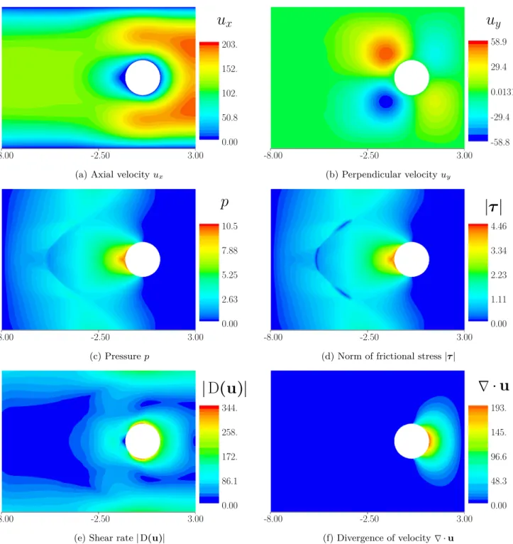
In our results section, we shall see that relaxing the common incompressibility assumption ∇ ⋅ u = 0 pre-vents the arising of an ill-defined rheology in some typ-ical scenarios such as the flow in the wake of an obsta-cle [Chauchat and Médale, 2014]. Moreover our comple-mentarity constraint (2) naturally fits in with our nu-merical framework, without adding any computational cumbersomeness.
3.1.3 Cases covered by our choice of rheology
Much like in [Ionescu et al., 2015], our set of parameters allows us to explore an interesting range of constitutive laws. When µ= 0, we retrieve the viscoplastic Bingham rheology, while when taking η= 0 and σ0 = 0, we get a purely Coulomb plastic flow — or, in other terms, the
µ(I) rheology with a constant inertial number I.
The numerical method for the quasistatic simulation presented in Section4will require a non-zero η to obtain a well-posed system. However, this constraint will be alleviated in Section5 when using temporal schemes. In our numerical experiments, we were also able to simulate the complete µ(I) rheology by explicitly computing the inertial number I at each time step.
Note also that the σ0 coefficient should not be assim-ilated to the usual cohesion term. Indeed, in our case the additional stress due to this coefficient will always be tangential, and may be non-zero when∇ ⋅ u > 0. In this regard, σ0should rather be used to model effects related to the geometry of grains. If we were to model proper co-hesion c, we could do so by defining κ(p) ∶= µ(p + c), and the pressure unilateral constraint as 0≤ p + c ⊥ ∇ ⋅ u ≥ 0. However in the framework presented below, thanks to a change of variable this would be strictly equivalent to adding a positive confining pressure to the right-hand side of the conservation of momentum equation. In the following, we shall thus free ourselves from modeling such a cohesion effect explicitly.
3.1.4 Solution set DP (µ, σ0)
Let us introduce the symmetric tensor λ∶= 2η Db(u) −
σtot= pI − τ . Using the identities p = 1dTr(λ) and τ = − Dev λ, and the definition of D(u), our Drucker-Prager rheology (1—2) can be directly rewritten as
⎧⎪⎪⎪ ⎪⎪⎪⎪⎪ ⎪⎪⎪⎪⎪ ⎪⎨ ⎪⎪⎪⎪⎪ ⎪⎪⎪⎪⎪ ⎪⎪⎪⎪ ⎩ Dev(λ) = −κµ,σ0( Tr(λ) √ 2d ) Dev(D(u)) ∣ Dev(D(u))∣ if Dev(D(u)) ≠ 0, (3a) ∣ Dev(λ)∣ ≤ κµ,σ0( Tr(λ) √ 2d ) if Dev(D(u)) = 0, (3b) 0≤ 1 dTr(λ) ⊥ Tr(D(u)) ≥ 0. (3c)
In the remainder of this paper, we shall denote by DP (µ, σ0) ⊂ Sd2 the set of tensors (λ; D(u)) ∈ Sd× Sd
satisfying (3).
3.2
Analogy with solid frictional contact
3.2.1 Solid Signorini-Coulomb law
(B) (A)
uN u
uT
e
Figure 1: Local contact basis, with normal and tangent subspaces.
We briefly recall the Signorini-Coulomb friction law in the case of two solid objects (A) and (B) with a single contact point, as illustrated in Figure 1. Let u∈ Rd be
the relative velocity between the two colliding objects,
u∶= uA− uB, and r∈ Rdbe the reaction force applied by
object (B) onto object (A). We suppose that the surface of contact is sufficiently smooth so that the normal e∈ Rd at the contact point can be uniquely defined.
Disjunctive formulation The Signorini-Coulomb law for contact with dry friction states that the couple(r, u) has to satisfy at least one of the following cases,
⎧⎪⎪⎪ ⎪⎪⎪⎪ ⎨⎪⎪ ⎪⎪⎪⎪⎪ ⎩ r= 0 and uN≥ 0 (Take-off) ∥rT∥ ≤ µ rN and u= 0 (Sticking) ∥rT∥ = µ rN and { uN= 0 ∃α > 0, uT= −αrT (Sliding) (4) where xN ∈ R and xT∈ R
d−1 are the normal and
tangen-tial components of vector x ∈ Rd, respectively, µ is the
coefficient of friction at contact point, and∥ ⋅ ∥ is the Eu-clidean norm on Rd. Let us denote by C (µ) ⊂ Rd× Rd the set of (r, u) satisfying (4).
Functional formulations Though classical, the dis-junctive formulation (4) is not always the most conve-nient to work with in a numerical setup. Typically, one may prefer to express the Signorini-Coulomb law as a root-finding problem, i.e., in the form
(r, u) ∈ C (µ) ⇐⇒ f(r, u) = 0, (5) where f is a nonsmooth function from Rd× Rd
to Rd.
One classical example of such a nonsmooth function was notably provided by Alart and Curnier [Alart and Curnier, 1991], and defined as
fAC ∶ R d× Rd Ð→ Rd (r, u) z→ ( ΠR+(rN− ξNuN) − rN ΠBd−1(µrN)(rT− ξTuT) − rT ) ,
where ΠC is the orthogonal projection operator on the
convex spaceC, ξTand ξNare positive real numbers, and
Bd−1(a) ⊂ Rd−1is the ball of radius a≥ 0 centered at the
origin.
Another well-known function satisfying (5)
may be derived based upon De Saxcé and
Feng [De Saxcé and Feng, 1998]’s work. Indeed, thanks to their proposed change of variable, ˆu = u + µ∥uT∥ e,
the Coulomb law may be written compactly as Kd
1
µ ∋ ˆu ⊥ r ∈ K
d
µ, (6)
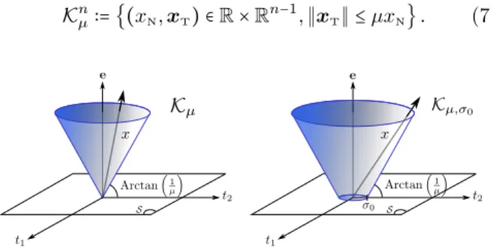
where the complementarity notation refers to the stan-dard orthogonality in Rd, and where Kµd ⊂ Rd is the second-order cone (SOC) of aperture µ (see Figure 2, left), generally defined on Rn (n≥ 2) as
Kn
µ∶= {(xN, xT) ∈ R × R
n−1,∥x
T∥ ≤ µxN} . (7)
Figure 2: The second-order cone (left) and the truncated second-order cone (right) represented in 3D (n= 3).
Now, let us recall the definition of the normal cone to a convex setC ⊂ Rn at point x∈ Rn,
NC(x) ∶= {y ∈ R n , y⊺(z − x) ≤ 0 ∀z ∈ C} if x∈ C NC(x) ∶= ∅ if x∈ R n− C. (8) Note that for an interior point x ∈ Int C, we have NC(x) = {0}. Moreover, in the particular case when
C has a smooth boundary, then on each point x of
the boundary BdC, the normal cone is spanned by the outward normal nC(x) to C at x, i.e., NC(x ∈ Bd C) =
{α nC(x), α ∈ R+}.
Let ξ be a positive scalar, x ∈ Rn and
y ∈ Rn. From the projection theorem (see, e.g., [Hiriart-Urruty and Lemaréchal, 2001, Proposition A.5.3.3]), we have
ΠC(x − ξy) = x ⇐⇒ y ∈ −NC(x) . (9)
In the particular case where C= Knµ, we have moreover
y∈ −NC(x) ⇐⇒ K n 1 µ ∋ y ⊥ x ∈ K n µ. (10)
Based on (6), (9) and (10), one may then derive the so-called De Saxcé function satisfying (5),
fDS ∶ R
d× Rd Ð→
Rd (r, u) z→ ΠKdµ(r − ξ ˆu) − r,
where ξ is a positive real number.
In Section 3.2.3 we will show that extended versions of both the Alart-Curnier and De Saxcé functions will play a similar role for our continuum granular rheol-ogy DP (µ, σ0). But since the above contact problem only involves the canonical Euclidean space Rd, we first need to introduce some mathematical tools in order to transpose it to the space of symmetric tensors.
3.2.2 Preliminary tools
Recall that Sd is the space of d× d symmetric tensors.
Let s(d) ∶= dim Sd = d(d+1)
2 . The dimension of the
hy-perplane of traceless tensors in Sd is t(d) ∶= s(d) − 1 =
(d − 1)(1 + d
2).
Definition 1. Let us introduce the morphism χ,
χ∶ R × Rt(d)→ Sd (a; b, c) ↦ ( bc −b ) +c a I if d= 2 (a; b, c, d, e, f) ↦ ⎛⎜⎜ ⎝ b−√c 3 d e d −b −√c 3 f e f √2c 3 ⎞ ⎟⎟ ⎠ + √ 2 √ 3a I if d= 3.
The morphism χ satisfies the following two properties, whose corresponding proofs are given inA.1.
Property 1. χ is an orthonormal isomorphism between
the two Euclidean spaces (Rs(d);⋅⊺⋅) and (S
d;< ⋅, ⋅ >).
This means
∀(x, y) ∈ Rs(d)× Rs(d)x⊺
y=< χ(x), χ(y) > , (11)
where x⊺
y is the usual scalar product on Rm, m≥ 1 and
< σ, τ >= σ∶τ
2 is our scalar product on Sd.
Property 2. Let us use the notation (σN; σT) ∶= σ ∶=
χ−1(σ) to decompose a symmetric tensor σ ∈ S
d or its
preimage by χ, σ∈ Rs(d), into a normal component σ
N∈ R and a tangential component σT∈ Rt(d). We have
1 √ 2dTr(σ) = σN and ∣ Dev(σ)∣ = ∥σT∥. (12a) (12b)
3.2.3 Reformulation of our rheology DP (µ, σ0) on Rs(d)
Thanks to our isomorphism χ, our Drucker-Prager rhe-ology DP (µ, σ0) (see Section 3.1.4), initially expressed on the tensorial space Sd, can be reformulated on Rs(d).
Theorem 1. Using the notations of Property2, the rhe-ology DP (µ, σ0) can be equivalently expressed as
⎧⎪⎪⎪ ⎪⎪⎪ ⎨⎪⎪ ⎪⎪⎪⎪ ⎩ λT= −κµ,σ0(λN) D(u)T ∥ D (u)T∥ if D(u)T≠ 0 (13a) ∥λT∥ ≤ κµ,σ0(λN) if D(u)T= 0,(13b) 0≤ λN⊥ D(u)N≥ 0, (13c) that is, (λ; D(u)) ∈ DP (µ, σ0) ⇐⇒
(λ; D(u)) satisfies Problem (13). (14) Problem (13), which now depends on vector variables, looks very similar to the disjunctive formulation (4) of the Coulomb friction lawC (µ) between discrete bodies, where λ plays the role2of the reaction force r, and D(u) that of the relative velocity u. Actually we shall see in the following section that in the special case where our fluid rheology is considered to be bidimensional (d= 2) and where σ0 = 0, Problem (13) then becomes exactly equivalent to the tridimensional discrete lawC (µ).
3.2.4 Functional formulations of our rheology
DP (µ, σ0) on Rs(d)
In this section, we show that similar functional formula-tions as those introduced in Section3.2.1for the solid con-tact lawC (µ) do apply to our fluid rheology DP (µ, σ0). The corresponding proofs are given inA.2.
Extended Alart-Curnier formulation
Definition 2. Let us introduce the following extension
of the Alart-Curnier function f⋆
AC, Rs(d)× Rs(d) → Rs(d)
(λ, D(u)) ↦ ( ΠR+(λN− ξND(u)N) − λN ΠBt(d)(κ(λ
N))(λT− ξTD(u)T) − λT )
where ξTand ξNare positive real numbers, andBt(d)(a) ⊂
Rt(d) is the ball of radius a≥ 0 centered at the origin.
Theorem 2. The following equivalence holds,
(λ; D(u)) ∈ DP (µ, σ0) ⇐⇒ fAC⋆(λ, D(u)) = 0. (15)
Extended De Saxcé formulation Let n ≥ 2. Let Kn
µ,σ0 be the truncated version of the SOCK
n µ already defined in (7), Kn µ,σ0∶= {(xN, xT) ∈ R+× R n−1,∥x T∥ ≤ σ0+ µxN} . (16)
See Figure2, right, for an illustration in the case when
n= 3. Note that similarly to Knµ, the setKnµ,σ0 is convex, and for σ0= 0 we recover Kµ,σn 0= K
n µ.
2Note however that the tangential counterparts of λ and r, and of D(u) and u respectively, do not share the same dimension. For instance, when d = 3, λT∈R5 and D (u)T∈R5 while rT∈R2 and
uT∈R2.
Let us apply a similar change of variable to De Saxcé’s [De Saxcé and Feng, 1998] on our symmetric velocity gradient tensor D(u), ˆD (u) ∶= D(u) + √
2
dµ∣ Dev(D(u))∣ I. Using (12) and the linearity of the
trace operator on the one hand, the linearity of the ()T operator and the fact that IT = 0 on the other hand, we
get
ˆ
D(u)N= D(u)N+ µ∥ D (u)T∥ ˆ
D(u)T= D (u)T.
(17a) (17b) Similarly to the modified solid velocity ˆu∈ Rdintroduced in Section3.2.1, which automatically lies in the polar cone Kd
1
µ
when uN≥ 0, our quantity ˆD (u) ∈ R1+dT has an
un-changed tangential component and a normal component that is modified such that ˆD(u) ∈ Ks(1d)
µ
when D(u)N≥ 0 (see Equivalence (47a)).
Definition 3. Let us introduce the following extension
of the De Saxcé function, f⋆
DS ∶ Rs(d)× Rs(d) Ð→ Rs(d)
(λ, D(u)) z→ ΠKs(d)
µ,σ0(λ − ξ ˆD (u)) − λ
(18)
where ξ is a positive real number.
Theorem 3. The following equivalence holds,
(λ; D(u)) ∈ DP (µ, σ0) ⇐⇒ fDS⋆(λ, D(u)) = 0. (19)
Corollary 1. When σ0= 0, the rheology DP (µ, σ0) can
be expressed as a Second-Order Cone Complementarity Problem (SOCCP), (λ; D(u)) ∈ DP (µ, 0) ⇐⇒ Ks(d) µ ∋ λ ⊥ ˆD (u) ∈ K s(d) 1 µ , where the ⊥ notation refers to Euclidean orthogonality in
Rs(d).
4
Creeping flow
4.1
The continuous setting
In this first section we assume that the flow is slow enough for its inertia to be neglected, and solve for its steady state. This case is relevant since the structure of the equations for each time-step of the fully dynamic case will be similar (see Section5).
Let us consider a domain Ω ⊂ Rd and decompose its boundary as ∂Ω ∶= BD∪ BN, with Dirichlet boundary
conditions on BD and homogeneous Neumann on BN,
u= uD on BD
Db(u) nΩ= 0 on BN
(20a) (20b) where nΩ is the outward-pointing normal to Ω on each point of its boundary.
Moreover, let σext gather all external stresses applied
onto the Neumann boundary of the domain. We thus have
−λ nΩ= σextnΩ on BN (21)
Conservation of momentum gives
−∇ ⋅ ⎡⎢ ⎢⎢ ⎢⎢ ⎢⎢ ⎣ 2η Db(u) − λ ´¹¹¹¹¹¹¹¹¹¹¹¹¹¹¹¹¹¹¹¹¹¹¹¹¹¹¹¹¹¹¹¸¹¹¹¹¹¹¹¹¹¹¹¹¹¹¹¹¹¹¹¹¹¹¹¹¹¹¹¹¹¹¹¶ =σtot ⎤⎥ ⎥⎥ ⎥⎥ ⎥⎥ ⎦ = ρgeg on Ω (22)
with eg the “down” unit vector.
Dimensionless equations Let L be a characteristic dimension of the flow. We define U∶=√gL the
character-istic velocity and P ∶= ρgL the characteristic pressure of the flow. We consider dimensionless differential operators defined through ˜∇ ∶= L ∇. We furthermore introduce two dimensionless numbers, the Reynolds number Re∶= ρU Lη and the Bingham number Bi∶= σ0
ρgL= σ0
P.
Considering the dimensionless quantities ˜u∶= U1u, ˜τ∶=
1
Pτ , ˜λ∶= P1λ, and ˜uD∶= U1uD, Equations (20—22) can
be made dimensionless as ⎧⎪⎪⎪ ⎪⎪⎪⎪⎪ ⎨⎪⎪ ⎪⎪⎪⎪⎪ ⎪⎩ −˜∇ ⋅ [ 2 ReD̃ b(˜u) − ˜λ] = e g on Ω ˜ u = ˜uD on BD ̃ Db(˜u) nΩ = 0 on BN −˜λ nΩ = ˜σextnΩ on BN, (23)
with the dimensionless rheology
(˜λ; ˜D (˜u)) ∈ DP (µ, Bi) . (24)
Proof. By noting that ˜D(˜u) = LUD(u) and L2ηU2ρg = Re2,
Equations (23) can be obtained from (20 — 22) by di-rect calculation. As for the dimensionless granular rhe-ology (24), it directly follows from (13) by noting that
1
Pκµ,σ0(λN) = κµ,Bi(˜λN), and that, again,
complementar-ity is insensitive to positive scaling factors.
In the remainder of this article, unless otherwise men-tioned we shall use the dimensionless quantities and omit the tildes. In particular, from now we shall use the no-tation(λ; D(u)) ∈ DP (µ, Bi) for denoting our granular rheology.
4.2
Variational formulation
Let H1(Ω)d be the usual Sobolev space containing square-integrable functions from Rd × R to Rd, with square-integrable gradients. As in [Saramito, 2015, Ap-pendix A], we introduce the subspace V(uD) of H1(Ω)d
for which the Dirichlet boundary condition (20a) is sat-isfied, i.e.,
V(uD) = {u ∈ H1(Ω)d; u= uD on BD}
and the subspace V(0) of H1(Ω)d for which the
homo-geneous Dirichlet boundary condition is satisfied, i.e.,
V(0) = {v ∈ H1(Ω)d; v= 0 on BD}.
Let T(Ω) be the space of square-integrable symmetric tensor fields on Ω.
Proposition 1. A weak form of System (23 — 24) amounts to finding u ∈ V (uD), λ ∈ T (Ω), and γ ∈ T (Ω),
such that ⎧⎪⎪⎪ ⎪⎨ ⎪⎪⎪⎪ ⎩ a(u, v) = b(λ, v) + l(v) ∀v ∈ V (0) m(γ, τ ) = b(τ , u) ∀τ ∈ T (Ω) (λ; γ) ∈ DP (µ, Bi) , (25a) (25b) (25c)
where ∀x, y ∈ H1(Ω)d and ∀σ, τ ∈ T (Ω), a(x, y) and m(σ, τ ) are the symmetric positive-definite bilinear forms on H1(Ω)d×H1(Ω)dand T(Ω)×T (Ω), respectively,
a(x, y) = 2 Re ∫ΩD 0(x) ∶ D0(y) +b d(∇ ⋅ x) (∇ ⋅ y) m(σ, τ ) = ∫ Ωσ∶ τ ,
b(τ , x) is the bilinear form on T (Ω) × H1(Ω)d,
b(τ , x) = ∫
ΩD(x) ∶ τ , and l(x) is the linear form on H1(Ω)d,
l(x) = ∫
Ωeg⋅ x − ∫BN
(σextnΩ) ⋅ x
Proof. First, let us consider the stress boundary
condi-tion (21). One solucondi-tion would be to enforce it strongly, by discretizing λ over the subspace of T(Ω) which satisfy (21). However, this may lead to difficulties in the dis-cretization of the DP (µ, Bi) rheology. In our proposed implementation, we chose instead to allow in the inte-gration of the term∇ ⋅ σtotfor a possibly non-zero jump
JσtotK of the stress on BN.
Let us now derive the variational formulation for Sys-tem (23). We assume u∈ V (uD), and λ ∈ T (σext), and
let v ∈ V (0) be a test function. In this setting, mul-tiplying both sides of (23) by v and integrating over Ω yields − ∫Ω∇ ⋅ ( 2 ReD b (u) − λ) ⋅ v + ∫B N JσtotKnΩ⋅ v = ∫ Ωeg⋅ v. (26) Using the Green formula with the (20b) boundary con-dition for u and the homogeneous Dirichlet concon-dition for
v, a(u, v) = 2 Re ∫ΩD 0(u) ∶ D0(v) + b d(∇ ⋅ v) (∇ ⋅ u) = ∫ΩRe2 Db(u) ∶ D(v) = − ∫Ω(∇ ⋅ 2 ReD b(u)) ⋅ v (27)
and ∫Ω∇ ⋅ [λ] ⋅ v + ∫B N JσtotKnΩ⋅ v = − ∫ BN σextnΩ⋅ v − b(λ, v). (28) By combining (26 – 28) and the definition of l, we re-trieve (25a).
Let us now focus on the rheology DP (µ, Bi) given in (24), which contains inequalities that cannot be put directly under weak form. To circumvent this difficulty, we introduce an auxiliary variable γ∈ T (Ω) that weakly satisfies γ= D(u), i.e.,
∫ΩD(u) ∶ τ = ∫
Ωγ∶ τ ∀τ ∈ T (Ω), (29)
which is exactly equation (25b). We can thus express the rheologyDP (µ, Bi) under the weak form as (25b — 25c).
Remark Note that we do not include any additional equation ensuring the well-posedness of our system, such as the zero-average pressure condition which is commonly used for Stokes flows. Indeed, for a given velocity field, the DP (µ, Bi) rheology imposes the value of λ in the yielded regions, serving as an intrinsic boundary condi-tion for the stress field inside the rigid zones.
4.3
Discretization by Finite Elements
(FEM)
4.3.1 Discretization of the symmetric tensor fields
For the discretization of the space T(Ω), we shall make use of Lagrange FEM, that is all symmetric tensor fields will be expressed as functions of Ω, built as an interpola-tion of their values at the n degrees of freedom xi.
Let Qh be a finite-dimensional subspace of L2(Ω) of
dimension n. Let (αi)1≤i≤n be a basis of Qh, such that
αi(xj) = δi,j. Let (ej)1≤j≤s(d) be the canonical basis for
Rs(d). Then(αααs(kd))1≤k≤s(d) n, defined as
∀x ∈ Ω, αααs(d)
s(d) (i−1)+j(x) ∶= αi(x) ej for {
1≤ i ≤ n 1≤ j ≤ s(d) is a natural basis for Qs(hd). Finally, we may build a finite subspace Th⊂ T (Ω) from the basis (σσσk)1≤k≤s(d) ndefined
as
∀x ∈ Ω, σσσs(d) (i−1)+j(x) ∶= αi(x)χ(ej) for {
1≤ i ≤ n 1≤ j ≤ s(d) where our orthogonal isomorphism χ from Rs(d) to Sd
has been formerly introduced in Definition 1. We have the following relationship between the two bases(αααs(d))k
and(σσσ)k,
∀x ∈ Ω, χ (αααs(d)
k (x)) = σσσk(x) for 1≤ k ≤ s(d) n.
(30) Now, for λ and γ two symmetric tensor fields in T(Ω), let λh, γh ∈ Th be their corresponding discretized
func-tions built by interpolation at the n degrees of freedom
xi. Let ΛΛΛh and ΓΓΓh be the vectors of the (scalar)
co-efficients of the decomposition of λh and γh,
respec-tively, in the basis(σσσ)k. That is, λh(x) = ∑kΛΛΛh,kσσσk(x),
and γh(x) = ∑kΓΓΓh,kσσσk(x). Note that using (30),
functions λh and γh decompose on the basis (αααs(d))k
with exactly the same coefficients, that is λh(x) =
∑kΛΛΛh,kααα
s(d)
k (x), and γh(x) = ∑kΓΓΓh,kααα
s(d)
k (x). Thus,
since αααs(s(d)d) (m−1)+j(xi) = δi,mej, each vector of s(d)
coef-ficients ΛΛΛh[i] ∶= {ΛΛΛh,s(d) (i−1)+j, 1≤ j ≤ s(d)} corresponds
to the value λh(xi), and the decomposition of λh(x) on
the scalar basis(α)i reads λh(x) = ∑iΛΛΛh[i] αi(x).
Simi-larly, we have ΓΓΓh[i] = γh(xi) and γh(x) = ∑iΓΓΓh[i] αi(x).
From (19) and using the aforementioned properties, we may express our discrete granular rheology at each degree of freedom xi,1≤i≤n as
(λh(xi); γh(xi)) ∈ DP (µ, Bi) ⇐⇒ fDS⋆ (ΛΛΛh[i],ΓΓΓh[i]) = 0.
(31)
4.3.2 Discretization of the (bi)linear forms
Let Uh⊂ H1(Ω)d be a finite-dimensional vectorial space,
and Vh⊂ Uh its subspace satisfying the Dirichlet
bound-ary conditions
Vh(uD) ∶= {vh∈ Uh, vh= uDhon BD} ,
where uDhis the approximated (discrete) value of uDon
the FEM mesh. Let u∗
Dh∈ Uhbe the unique function such
that for any uh∈ Vh(uD), u∗Dh= uh− ΠVh(0)(uh), where
we recall that ΠC is the orthogonal projection operator
onto the convex setC.
Unlike for the space Th, here we make no specific
as-sumption regarding the structure of Vh(uD) or the
con-struction of a corresponding base. Let v∶= dimVh. Given
(vvvi)1≤i≤v a basis of Vh(0), we denote by A, B, and M
the matrices corresponding to the decomposition of the bilinear forms a, b, and m respectively, and by l the vector corresponding to the decomposition of the lin-ear form l. More precisely, we have Ai,j = a(vvvi, vvvj),
Mk,` = m(σσσk, σσσ`), Bk,j = b(σσσk, vvvj) and lj = l(vvvj).
Sim-ilarly, let Uh be the vector of scalar coefficients
corre-sponding to the decomposition of uh. We have, ∀x ∈ Ω,
4.3.3 FEM discrete system
Finally, at this point the discrete version of Equations (25a—25c) reads: Find uh∈ Vh(uD), (λh, γh) ∈ Th2,
⎧⎪⎪⎪ ⎪⎪⎪⎪⎪ ⎨⎪⎪ ⎪⎪⎪⎪⎪ ⎪⎩ A Uh= B⊺ΛΛΛh+ l − aD ´¹¹¹¹¹¸¹¹¹¹¶ ltot M ΓΓΓh= B Uh+ k (λh; γh) ∈ DP (µ, Bi) (32a) (32b) (32c) where for 1 ≤ i ≤ v, aD,i = a(u∗Dh, vvvi) and for 1 ≤ k ≤
s(d) n, kk= b(σσσk, u∗Dh).
4.3.4 Discretization of the rheology on quadra-ture points
In the discrete case, the nonsmooth rheologyDP (µ, Bi) will not hold at every point x∈ Ω, but only in the weak sense, i.e., on the space Th. That is, we replace (32c)
with
∫Ωf⋆
DS(λ, γ) ∶ τ = 0 ∀τ ∈ Th. (33)
We shall thus restrict ourselves to a discrete number of points ˘xj on which to enforce (λh(˘xj); γh(˘xj)) ∈
DP (µ, Bi). The remaining question is how to perform a good choice for this set of points ˘xj. In the sequel we
shall see that this choice has a direct impact onto the final form of the system to be solved, and thus on both the physical relevance of the discrete problem and the practical performance of available solving methods.
Discretization on Qh’s Lagrange degrees of
free-dom One obvious choice for (˘x)j is to consider the n degrees of freedom xi themselves, which served to define
the(α)i basis and thus the finite-dimensional spaces Qh
and Th. This way, using (31) we may replace (33) with
f⋆
DS(ΛΛΛh[i],ΓΓΓh[i]) = 0 for 1 ≤ i ≤ n.
Since A and M are positive-definite, we may first elim-inate the velocity variable Uh from (32a), and then get
a linear relationship between ΛΛΛh and ΓΓΓh from (32b),
Γ
ΓΓh ∝ M−1W ΛΛΛh where W = BA−1B⊺. Apart from the
presence of the matrix M which yields a modified De-lassus operator ˜W ∶= M−1W , we have thus obtained a
system which is very similar to the one appearing in dis-crete contact mechanics, and for which a plethora of ef-ficient solving methods exist [Cadoux, 2009]. However, the presence of the matrix M breaks the symmetry of the operator ˜W (M and W do not commute in the
gen-eral case). The discrete system (32) therefore lacks a fundamental symmetry property, which is key not only to guarantee physical consistency of our model, but also to design an efficient numerical solver.
From a physical point of view, such an asymmetry in our discrete frictional contact law typically implies that the maximum dissipation principle cannot be satisfied, meaning that some anisotropy is artificially introduced through the discretization.
From a purely numerical point of view, symmetry of the Delassus operator is not necessarily a prereq-uisite to common numerical solvers, but in our case it proves to be highly desirable for coming up with a tractable solving method. Indeed, among scal-able availscal-able solvers, we basically have the choice between operator-splitting algorithms (such as the well-known nonsmooth contact dynamics (NSCD) method [Jourdan et al., 1998]), and optimization-based algorithms (e.g. [Renouf and Alart, 2005, Cadoux, 2009]). On the one hand, operator-splitting methods do not assume W be symmetric, yet for˜
efficiency purposes they require the explicit knowledge of ˜W , especially when large systems are involved as it
is the case here. In our case A−1 is dense, and so is
˜
W . Making such an explicit assembly thus turns out to
be intractable. On the other hand, optimization-based methods do not require the explicit assembly of W ,˜
however they heavily rely upon its symmetry so as to identify ΓΓΓh as the gradient of a quadratic function in ΛΛΛh
with Hessian ˜W .
For these two reasons, we choose to discretize our con-straints on an alternative set of points (˘x)j that will allow us to eliminate the matrix M and thus retrieve symmetry of ˜W . This way we shall both recover
phys-ical consistency of our model, and benefit from efficient optimization-based solving methods.
Discretization on quadrature points As we are us-ing a Lagrange FEM discretization of the space T(Ω) with polynomial interpolating bases, each integral Mk,`=
∫ σσσk ∶ σσσ` can be computed exactly using Gaussian
quadrature3, i.e., as ∑qwq (σσσk(ˆxq) ∶ σσσ`(ˆxq)) where the
ˆ
xq,1≤j≤nQare the so-called quadrature points and wqtheir corresponding weights. As shown below, defining the set (˘x)q as the set of quadrature points ˆxq allows us to
retrieve a symmetric Delassus operator.
Recall that for λ a symmetric tensor field in T(Ω), λh∈
Thcorresponds to its discretized version interpolating the
values at the n degrees of freedom xm, with λh(xm) =
Λ Λ
Λh[m]. Let R be the (s(d) nQ× s(d) n) matrix mapping
those ΛΛΛh[m] to the interpolated values λh(˘xq) at the
quadrature points ˘xq. That is, R is such that
˘
ΛΛΛh= RΛΛΛh,
where ˘ΛΛΛh is the vector of size s(d) nQ concatenating the
nQ vector values ˘ΛΛΛh[q] ∶= λh(˘xq) for 1 ≤ q ≤ nQ, and ΛΛΛh
the vector of size s(d) n concatenating the n vector values Λ
Λ
Λh[m] = λh(xm) for 1 ≤ m ≤ n.
Matrix R contains nQ× n square blocks Rq,j of size
s(d) × s(d) with Rq,j= αj(˘xq) Is(d)for all 1≤ q ≤ nQ and
1 ≤ j ≤ n, where Is(d) is the s(d) × s(d) identity block.
This translates into the following elementwise expression
R(q−1)s(d)+p,(j−1)s(d)+`= αj(˘xq)δp,` for 1≤ p, ` ≤ s(d). 3Of course each coefficient M
k,`may alternatively be evaluated
by direct integration, since primitives of the integrand are easily calculable. However, the quadrature technique is mentioned here as it provides a judicious set of points on which to discretize our rheology.
Property 3. Let ˘ΛΛΛh ∶= RΛΛΛh and ˘ΓΓΓh ∶= RΓΓΓh, and R†
the Moore-Penrose pseudoinverse of R. Then Equations (25a— 25c) can be discretized as:
Find Uh∈ Rv, ˘ΛΛΛh, ˘ΓΓΓh∈ Rs(d) nQ, ⎧⎪⎪⎪ ⎪⎪⎪ ⎨⎪⎪ ⎪⎪⎪⎪ ⎩ A Uh= B⊺R†ΛΛΛ˘h+ ltot ˘ Γ Γ Γh= R†,⊺B Uh+ R†,⊺ktot ∀1 ≤ q ≤ nQ, fDS⋆ (˘ΛΛΛh[q], ˘ΓΓΓh[q]) = 0. (34a) (34b) (34c)
The corresponding proof is given inA.3.
This time we have obtained in (34) a system which pre-serves the symmetry of the new Delassus operator ˘W = R†,⊺B A−1B⊺R†. One remaining difficulty stems from
the presence of the matrix R†, which in the general case could increase substantially the cost of solving the sys-tem.
4.3.5 Considerations on R†
Trapezoidal quadrature rule The first observation is that if the quadrature points (˘xq) were to coincide
with the degrees of freedom (xi), R would boil down to
the identity matrix and the operator R†would not induce any additional cost. This is actually always the case for a piecewise constant (P0) approximation, for which both the degrees of freedom and the quadrature points are lo-cated at the barycenter of each element.
For higher-order polynomial basis functions, having the (˘x)q coincide with the (x)i amounts to computing
m(γ, τ ) using a trapezoidal integration rule. Obviously,
such an approximation induces a loss of precision — the integral being exact only for functions that are linear be-tween the degrees of freedom. This means that the order of convergence will not increase with that of the basis functions, and using high-order discretization space (P2
or higher-order polynomials) would be wasteful. How-ever, for piecewise linear (P1) polynomials, we found such approximation to be acceptable, and used it in practice.
Mixed finite elements In the case of piecewise-polynomial discontinuous basis functions, degrees of free-dom are not shared between adjacent elements. When considering such a discretization of the space T(Ω), the matrix R becomes block-diagonal, and consequently its pseudo-inverse has a similar structure and is easy to com-pute. The additional cost induced by the presence of the linear operator R†in Problem (34) is therefore once again negligible.
4.3.6 Final discrete system
For brevity of notation and since there are no more am-biguities, from now on we shall drop the decorations and capitalization of the variables, i.e., we shall consider Problem (34) written as:
Find u∈ Rv, λ, γ∈ Rs(d) nQ, ⎧⎪⎪⎪ ⎪⎪ ⎨⎪⎪ ⎪⎪⎪⎩ A u= B⊺R†λ+ l γ= R†,⊺B u+ R†,⊺k 0= f⋆ DS(λ, γ), (35a) (35b) (35c) where f⋆ DSis extended from R s(d) to RnQs(d) by concate-nation.
4.4
Solving (
35
) numerically in the case
Bi = 0
In the case when Bi = 0, from Corollary 1 the con-straint (35c) boils down to K1
µ ∋ ˆγ ⊥ λ ∈ Kµ. The re-sulting problem was extensively studied in the contact mechanics field, see e.g., [Cadoux, 2009] for a review.
4.4.1 Cadoux’s algorithm
Several methods have been proposed to decompose Problem (35) as a succession of optimization prob-lems depending on a varying parameter s, see e.g. [Haslinger and Tvrd`y, 1983, Renouf and Alart, 2005, Acary et al., 2011]. We recall in this section the fixed-point algorithm originally presented in [Cadoux, 2009, Acary et al., 2011], which allows us to rewrite our problem as a nested loop of Second-Order Cone Quadratic Problems (SOCQP). The advantage of this algorithm over most other iterative approaches is that the successive values of the parameter s depend only on the primal variable u; each intermediate SOCQP will have a unique solution in u, but may admit a continuum of solutions in the dual variable λ.
First, let us introduce the reduced (or dual) version of Problem (35), which is derived by eliminating the velocity variable u,
W λ+ w = γ λ, γ ∈ R2s(d) nQ
f⋆
DS(λ, γ) = 0,
(36)
where W = R†,⊺BA−1B⊺R† and w= R†,⊺(BA−1l+ k).
For any value of a parameter s ∈ RnQ
+ , we define the quadratic function Js(λ) ∶= 1 2λ ⊺ W λ+ λT(w + (s; 0))
and the SOCQP
min
λ∈Kµ
Js(λ). (37)
Corresponding optimality conditions readK1
µ ∋ ∇Js(λ) ⊥
λ∈ Kµ, i.e.,
K1
µ ∋ γ + (s; 0) ⊥ λ ∈ Kµ. (38) Let us introduce the mappings v ∶ RnQ
+ → R
s(d) nQ, s ↦
v(s) ∶= ∇Js(λ∗(s)) with λ∗(s) a solution to the
SOCQP (37), and F ∶ RnQ
+ → R
nQ
+ , s↦ µ∥v(s)T∥.
Acary et al., 2011] show that v and therefore F are uniquely defined.
Solving our problem amounts to finding a fixed-point
s∗ of F , thus setting λ= λ∗(s∗). Indeed s∗ = F (s∗) = µ∥γT+ (s∗; 0)
T∥ = µ∥γT∥, and therefore the KKT
condi-tions (38) yield K1
µ ∋ γ + (µ∥γT∥; 0) ⊥ λ ∈ Kµ. We identify ˆγ∶= γ + (µ∥γT∥; 0) and get f⋆
DS(λ, γ) = 0.
Data: λ initial guess Data: ε> 0 tolerance Result: (λ; γ) satisfying (36) Loop γ← W λ + w ; break if∣fAC(λ, γ)∣ < ε; s← µ∥γ∥ ; λ← solution of SOCQP (37) at s ; end
Algorithm 1: Fixed-point algorithm with
Alart-Curnier stopping criterion
F is not guaranteed to be a contraction; in
Sec-tion (4.4.5) we will present some sufficient condiSec-tions for the existence of a fixed point. In practice, we observe very good convergence of the fixed-point algorithm 1. More complex rules for iterating on s have been investigated in [Cadoux, 2009] but have not been found to perform significantly better.
4.4.2 Second Order Cone Programming
The easiest way to tackle the SOCQP (37) is to leverage the efficiency of out-of-the-box interior-points solvers for Second Order Cone Programs (SOCP), of which it is a subclass.
The first step consists in removing the quadratic part of the objective function by introducing a variable t∈ R subject to the constraint t≥12λ⊺
W λ. The new objective
is ˆJs(t, λ) = t + λT(w + (s; 0)).
Given a square root L of A, we have A = LL⊺ and W = (L−1BTR†)⊺L−1B⊺R†. With an auxiliary variable
y∈ Rvthat satisfies Ly= B⊺R†λ, the constraint on t now
reads 2t≥ y⊺y and may also be written as a rotated cone
constraint(1, t, y) ∈ RK. We obtain the SOCP
min t∈R,λ∈Rs(d) nQ t+ λ⊺(w + (s; 0)) Rz= λ Ly= B⊺ z λ∈ KnQ µ (1, t, y) ∈ K1. 4.4.3 Projected Gradient
The interior-point approach has some drawbacks: ar-guably, the reliance on a complex external code, but most importantly, the inability of interior-point solvers to be
warm-started. As our outer fixed-point loop converges, the quality of our initial guess increases and we would like the SOCQP solver to take advantage of this.
Another natural way to solve the SOCQP is to use an algorithm of the Projected-Gradient (or Projected Gra-dient Descent) families (PG). In its simplest form, such an algorithm reads:
Data: λ initial guess Data: Step length ξ> 0
Result: λ solution of SOCQP (37)
Loop y← W λ + w + (s; 0) ; x← ΠKµ(λ − ξy); break if∣x − λ∣ < ε; λ← x end
Algorithm 2: Projected Gradient Descent algorithm.
Since Algorithm (2) can converge quite slowly in prac-tice, several works have focused on finding ways to im-prove its speed, among which we note
• Performing a line-search of the step size ξ;
• The Accelerated Gradient Descent method from Nesterov [Nesterov, 1983], adapted to SOCQP in [Heyn, 2013];
• The Spectral Gradient method from Barzilai et al. [Barzilai and Borwein, 1988], adapted to
SOCQP in [Tasora, 2013].
Using such techniques, we found the PG method to be competitive with interior-points solvers on our problem, especially as the outer fixed-point loop converges and the quality of the initial guess increases. Numerical details are provided in Section 6.4.
4.4.4 Primal algorithm
In some situations, one may only be interested in the pri-mal variable u, and may not need the value of the dual variable λ. In this case, following [Cadoux, 2009] again, we can implement the fixed-point algorithm directly on the primal formulation, and avoid the need for some aux-iliary variables.
The insight is that the SOCQP (37) is the dual of another optimization problem, namely
min u∈C(s) J∗(u) (39) with J∗(u) ∶= 1 2u ⊺ Au− u⊺ l C(s) ∶= {u ∈ Rv, R†,⊺(Bu + k) + (s; 0) ∈ K1 µ} . In contrast to the dual (37), the SOCQP (39) is strictly convex, and therefore guaranteed to admit a unique so-lution as long as the feasible set is not empty.
Data: u initial guess Data: ε> 0 tolerance Result: u satisfying (35) Loop γ← R†,⊺(Bu + k) ; s← µ∥γ∥ ; u← solution of SOCQP (39) at s ;
break if successive iterates close enough; end
Algorithm 3: Primal version of the fixed-point
algo-rithm
Algorithm 1 can then be trivially adapted to use the primal minimization problem, as in Algorithm3. Due the to complex nature of the constraint, the SOCQP (39) is not suited for a Projected-Gradient algorithm, however it can be just as easily put under a SOCP form.
min t∈R,u∈Rvt− u ⊺ l R⊺ z= B u + k + R⊺(s; 0) y= L⊺ u z∈ KnQ 1 µ (1, t, y) ∈ K1 4.4.5 Existence of solutions
Criterions that ensure the existence of solutions to the discrete Coulomb friction problem, of which Prob-lem (35) is an instance, are given in [Cadoux, 2009, Acary et al., 2011]; we restate them below. Note that those criterions are only sufficient, and not necessary. First, the hypothesisH(µ),
H(µ) ∶= ∃u, R†,⊺(Bu + k) ∈ K1
µ, (40)
ensures the existence of a fixed-point s∗ of F , i.e., such
that s∗ = F (s∗). The velocity u is given by the unique
solution to the primal problem (39) at s∗, and the strain
rate tensor γ can be deduced from u. The existence of a corresponding stress field λ boils down to
∃λ ∈ Kµ, B⊺R†λ= A u − l and ˆγ⊺λ= 0
which is automatically satisfied under a stronger hypoth-esis,
H(µ) ∶= ∃u, R†,⊺(Bu + k) ∈ Int K1
µ. (41)
Proof. H(µ) yields directly that Int C(s) ≠ ∅. As u is a
solution of (39),−∇J∗(u) ∈ N
C(s)(u). We have
NC(s)(u) = ∂IC(s)(u) = ∂IK1
µ (R
†,⊺(Bu + k) + (s; 0))
whereIC(x) denotes the value of the characteristic
func-tion of the convex set C at x. As Int C(s) ≠ ∅, the latter subdifferential yields exactly
NC(s)(u) = BTR†∂IK1 µ (u) = B ⊺ R†NK1 µ (u) . Finally, we have NK1 µ(u) ⊂ −Kµ∩ {ˆγ} ⊥, and therefore A u− l = ∇J∗(u) ∈ B⊺R†(K µ∩ {ˆγ}⊥).
In the case µ= 0, the strong hypothesis H(µ) amounts to the existence of a velocity field with strictly positive divergence everywhere – this requires outward Dirich-let boundary conditions, or a Neumann boundary. The weakerH(µ) only requires that there exist a velocity field with nowhere strictly negative divergence.
Homogeneous Dirichlet boundary conditions only sat-isfy the latter, weaker criterion H(µ). However we can always exhibit a trivial solution in u, λ; for µ= 0, it cor-responds to the incompressible Stokes solution, and for
µ> 0, to the null velocity solution, u = 0.
Proof. By construction we have k= 0. Moreover, the
con-dition imposes ∫Ω∇ ⋅ u = ∫∂ΩuD⋅ n = 0. As the rheology
requires∇ ⋅ u ≥ 0, velocity solutions must have null diver-gence, which means in the discrete case(R†,⊺Bu)N= 0.
In the case µ = 0, s∗ = 0 is a fixed-point of F , and
the primal feasibility condition u ∈ C(0) boils down to (R†,⊺Bu)
N= 0. The optimality condition reads
−∇J∗∈ N
C(0)(u) = (Ker (R†,⊺B)N)
⊥= Im (R†,⊺ B)⊺N, so there exists λ with∇J∗= BTR†λ and λ
T= 0.
In the case µ> 0, u ∈ C(0) boils down to R†,⊺Bu= 0.
This means that the solution u∗(0) of the primal problem
at s = 0 satisfies ∥(B⊺R†u)
T∥ = 0, and therefore s ∗ = 0
is a fixed point of F . The optimality condition yields ∃λ, ∇J∗= BTR†λ.
In both cases, we define λ∗ ∶= λ + (∆
p; 0), with ∆p
constant over all discretization points. By construction,
λ−λ∗∈ Ker BTR†. We can choose ∆
psuch that λ∗∈ Kµ;
for µ= 0, it suffices to take ∆p∶= − min λN, and for µ> 0,
∆p ∶= − min(λN−µ1λT). We have then A u − l = ∇J ∗ = BTR†λ∗
, and it can be easily verified that ˆγ⊺
λ∗= 0.
4.5
Solving (
35
) numerically in the case
Bi > 0
The case Bi> 0, where the SOC Kµ is replaced with the
truncated one Kµ,Bi, has not been as extensively studied
in the literature. In the following sections, we show that we can extend the framework presented above to Bi > 0. Furthermore, a simple modification to the Projected-Gradient algorithm will be sufficient to solve our problem.
4.5.1 Duality
Theorem 4. We introduce a modification of the objective
function of the primal problem (39), J∗ Bi(u) ∶= J∗(u) + Bi nQ ∑ i=1 ∥(R†,⊺(Bu + k))i T∥,
and the two optimization problems,
min u∈C(s) J∗ Bi(u) min λ∈Kµ,Bi Js(λ). (42) (43)