A THESIS SUBMITTED IN PARTIAL FULFILMENT OF THE REQUIREMENTS FOR THE DEGREE
OF
DOCTOR OF PHYLOSOPHY IN ELECTRICAL ENGINEERING
By FANGHUI YIN
Modeling and Experimental Investigation of the Effects of Electric Field and Corona Discharge on Ice Accreted on High-Voltage Conductors
Modélisation et étude expérimentale des effets du champ électrique et des décharges de couronne sur l'accumulation de glace sur les conducteurs haute tension
Québec, Canada
ABSTRACT
Atmospheric icing affects a wide variety of man-made structures in many countries. It is generally well known to occur in countries like Japan, Canada, Iceland, Russia as well as China. When the power transmission lines are subject to icing, huge corona loss due to corona discharge or rupture of transmission lines may be caused because of the ice load. In the worst-case scenario, it would lead to power outage and collapse of tower.
The objective of this study is to investigate the effects of electric field and corona discharge on ice accreted on high-voltage conductor. The research was approached by two methods, experiments and simulations. To achieve this objective, experiments were carried out by means of a corona cage in a climate room at CIGELE laboratories, University of Quebec in Chicoutimi (UQAC) and the simulations were performed by a finite element software. Rime and glaze were considered in the present study as they are thought to be the most adverse conditions for power transmission lines.
The experimental results showed that the electric field has a significant influence on ice formation. Under both rime and glaze ice conditions, the weight of ice accreted on the surface of the conductor increased with electric field strength up to 20 kVrms/cm and then decreased as it is increased further. Without voltage applied on the conductor, about half of the total weight of glaze ice can be contributed by the icicle accretion. In the presence of electric field, the weight percentage of icicles could be lowered to 14%. When the water film was freezed right after they reached the bottom of the conductor, the icicle spacing was independent of electric field. If developed water pedants were formed before they were freezed, the icicle spacing decreased with an increase of electric field. Due to the repulsion force of the pendant drops at the icicle tip, the presence of electric field can result in an angle between adjacent icicles accreted on the conductor. This angle increased with an increase of conductor surface electric field.
The corona loss was mainly contributed by the fundamental component. The contribution of other harmonic components on corona loss can be neglected, except for the harmonic component which was already significant in the applied voltage. The power factor of the 3rd harmonics can be used to determine whether the
conductor is running below or above its corona onset voltage. If it was close to 0.5, the conductor was running near its corona onset voltage. If it was higher than 0.5, it can be expected that the conductor was operated beyond its corona onset voltage. According to the simulated results, it was found that when the electric field is no higher than 20 kVrms/cm, the ice accretion model works well. However, with the electric field increased further, the results diverged because of the generation of corona wind.
RÉSUMÉ
Le givrage atmosphérique affecte un éventail de structures dans beaucoup de pays, tels que le Japon, le Canada, l’Islande, la Russie et également la Chine. Les lignes de transport de l’énergie électrique soumises aux accumulations de glace peuvent subir d’importantes pertes d’énergie à la suite de décharges couronne ou de rupture des conducteurs. Dans le pire des cas, ceci peut dégénérer en coupures de courant et dans l’effondrement de pylônes.
L’objectif poursuivi par ce travail est l’étude des effets du champ électrique et des décharges couronne sur la glace accumulée sur les conducteurs à haute tension. Deux approches ont été utilisées dans cette recherche : l’approche expérimentale et la simulation numérique. Pour atteindre cet objectif, des expériences pratiques ont été effectuées en utilisant une configuration cylindrique montée dans une chambre climatique aux laboratoires de la CIGELE à l’université du Québec à Chicoutimi (UQAC). Quant aux simulations numériques, elles ont été réalisées par la méthode des éléments finis. Le givre lourd et le verglas ont été utilisés dans cette étude, car ces types de glace sont considérés comme les plus dangereuses pour les lignes de transport d’énergie électrique.
Les résultats expérimentaux ont montré que le champ électrique a un effet significatif sur la formation de la glace. Dans des conditions de givre ou de verglas, le poids de la glace accumulée à la surface du conducteur augmente avec l’intensité du champ électrique jusqu’à 20 kVrms/cm, pour ensuite diminuer si cette intensité augmente davantage. En l’absence de tension appliquée au conducteur, environ la moitié du poids total de verglas est attribuable à l’accumulation de glaçons. En présence d’un champ électrique, le pourcentage en poids des glaçons peut diminuer jusqu’à 14%. Lorsque le film d’eau gèle immédiatement après avoir atteint la surface inférieure du conducteur, l’espacement entre les glaçons devient indépendant du champ électrique. À cause de la force de répulsion des gouttes d’eau en suspension au bout des glaçons, la présence d’un champ électrique peut résulter en la formation d’un angle entre les glaçons adjacents accumulés sur le conducteur. Cet angle augmente avec l’accroissement du champ électrique à la surface du conducteur.
La perte en énergie due à l’effet couronne provient principalement de la composante fondamentale. La contribution des autres composantes harmoniques sur la perte couronne est négligeable, sauf pour la composante harmonique, qui était déjà significative dans la tension appliquée. Le facteur de puissance relatif à la 3e harmonique peut être utilisé pour déterminer si le conducteur est alimenté par une tension électrique plus basse ou plus élevé que la tension de seuil de l’effet couronne. Si le facteur de puissance est de 0.5, le conducteur est sous une tension près de la tension de seuil de l’effet couronne. S’il est supérieur à 0.5, on peut supposer que la conducteur est alimenté par une tension plus élevé que la tension de seuil de l’effet couronne. En se basant sur les résultats de la simulation, il a été observé que lorsque le champ électrique à surface du conducteur ne dépasse pas 20 kVrms/cm, le modèle d’accumulation de glace fonctionne adéquatement. Toutefois, si le champ électrique augmente davantage, les résultats divergent à cause de la génération de vent électrique.
TABLE OF CONTENTS
ABSTRACT ... ii
RÉSUMÉ ... iv
TABLE OF CONTENTS ... vi
LIST OF SYMBOLS ... ix
SYMBOL ... ix
CONCETP ... ix
DIMENSIONS ... ix
LIST OF TABLES ... xi
LIST OF FIGURES ... xii
ACKNOWLEDGMENTS ... xiv
CHAPTER 1 ... 1
INTRODUCTION ... 1
1.1
Definition of the problem ... 2
1.2
Research objectives ... 5
1.2.1 Experiments ... 5
1.2.2 Simulations ... 6
1.3
Methodology ... 6
1.4
Statement of the originality of the thesis ... 8
1.5
Thesis outline ... 8
CHAPTER 2 ... 10
REVIEW OF LITERATURE ... 10
2.1
Types of atmospheric icing accretion ... 11
2.1.1 Precipitation icing ... 11
2.1.2 In-cloud icing ... 14
2.1.3 Hoar frost ... 15
2.2
Corona loss ... 16
2.2.1 Electric power system ... 16
2.2.2 Conductor corona onset gradient ... 18
2.2.3 Conductor corona loss predication ... 19
2.3
Measurement methods for corona performance ... 21
2.3.2 Outdoor corona cage ... 25
2.3.3 Outdoor test lines ... 27
2.3.4 Operating lines ... 28
2.4
Development of numerical modelling for ice accretion ... 28
2.5
Conclusion ... 31
CHAPTER 3 ... 32
EXPERIMENTAL FACILITIES AND TEST PROCEDURES ... 32
3.1
Experimental facilities ... 33
3.1.1 Climate room ... 33
3.1.2 Corona cage ... 34
3.1.3 Data acquisition and processing system ... 37
3.2
Test procedure ... 39
CHAPTER 4 ... 46
THE INFLUENCE OF ELECTRIC FIELD STRENGTH ON ICE FORMATION ... 46
4.1
The influence of electric field strength on ice appearance ... 47
4.2
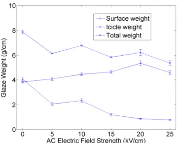
The influence of electric field strength on ice weight ... 49
4.3
The influence of electric field strength on icicle spacing ... 56
4.4
The influence of AC electric field strength and wind velocity on length of icicles ... 62
4.5
The influence of electric field strength on angle between adjacent icicles ... 64
4.6
Conclusion ... 68
CHAPTER 5 ... 69
THE INFLUENCE OF ELECTRIC FIELD STRENGTH ON CORONA
CHARACTERISTICS ... 69
5.1
The equivalent circuit representing the corona process ... 70
5.2
The influence of electric field strength on corona loss ... 72
5.3
The influence of electric field strength on corona onset voltage ... 81
5.4
The influence of electric field strength on leakage conductance ... 86
5.5
The influence of electric field strength on capacitance ... 88
5.6
The investigation of harmonics distortion ... 93
5.7
The effect of harmonics on corona loss ... 99
5.8
The dynamic characteristics of the 3
rdpower factor ... 103
CHAPTER 6 ... 113
ICE ACCRETION SIMULATION AND ITS EXPERIMENTAL VALIDATION ... 113
6.1
Ice accretion model ... 114
6.1.1 Model structure ... 114
6.1.2 Airflow computation ... 117
6.1.3 Droplet trajectory calculation ... 118
6.1.4 Collision efficiency calculation ... 122
6.1.5 Ice growth process... 124
6.2
Model simulation and validation ... 125
6.2.1 Comparison of accreted rime between experiments and simulations ... 126
6.2.2 The influence of wind velocity ... 135
6.2.3 The influence of water droplet diameter ... 136
6.3
Conclusion ... 137
CONCLUSIONS AND RECOMMENDATIONS ... 138
7.1
Conclusions ... 139
7.2
Recommendations ... 141
LIST OF SYMBOLS
SYMBOL CONCETP DIMENSIONS
a Droplet radius m
Cd Drag Coefficient
Cg Geometric capacitance F
Cn Non-linear capacitance F
Csc Stokes-Cunningham slip correction factor
CL Corona loss W/m
D Diameter of the conductor m
e Eccentricity
Ec Corona onset gradient kV/cm
Esurface Conductor surface gradient
f Frequency Hz
Fd Drag N
FDEP Dielectrophoretic force N
Gc Leakage conductance S
h Heat transfer coefficient W/(m2∙K)
i current A
IP Phase current A
m Conductor surface roughness
p Dipole moment (C∙m)
P Power per meter W/m
PRL Power of resistive loss W
rc Conductor radius m
rsc Sub-conductor radius m
R Radius of the outer cylinder m
Re Reynolds number
SD Standard deviation
THD Total harmonic distortion
u Votlage V
v Velocity m/s
V Voltage V
Vo Corona onset votlage V
w Liquid water content g/m3
Greek Symbols
ε Dielectric constant F/m
δ Relative air density
σ20 Water conductivity μS/cm
γ Surface tension N/m
η Fluid viscosity Pa∙s
ρ Density kg/m3
τ Relaxation time s
φ Bent angle of icicles
Φ Angle between adjacent icicles
σ Charge density C/m2
λ Mean free path m
LIST OF TABLES
Table 3-1: Temperature Coefficient at Different Temperatures ... 42
Table 3-2: Environmental Parameters... 42
Table 3-3: Surface Field Strength and Corresponding Voltage for the Tested Corona Cage Configuration .... 44
Table 4-1: Rime Weights on Conductor Surface at Different AC Electric Field Strengths with Wind Velocity of 2 m/s. ... 50
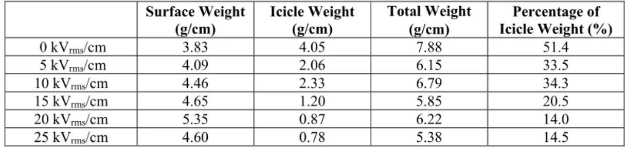
Table 4-2: Glaze Weights at Different AC Electric Field Strengths with Wind Velocity of 2 m/s. ... 50
Table 4-3: Distortion of Water Droplets by Background Electric Fields. ... 52
Table 4-4: Acceleration (m/s2) Component Induced by Electric Force at Various Distances from Conductor Surface. ... 54
Table 4-5: Spacings of Icicles (mm) at Different Electric Field Strengths. ... 57
Table 4-6: Diameters of Icicles at Root at Different Electric Fields. ... 61
Table 5-1: Comparison of Corona Losses after 40 Minutes of Rime Accretion at Different Wind Velocities. 74 Table 5-2: Comparison of Corona Losses after 40 Minutes of Glaze Ice Accretion at Different Wind Velocities... 75
Table 5-3: Comparison of Corona Losses Measured on a Transmission Line and Calculated Equivalent CLs Originated from Corona Cage. ... 78
Table 5-4: Corona Loss Conversion from Corona Cage to a 1000 kV AC test line when the side phase is subjected to various electric field strengths. ... 79
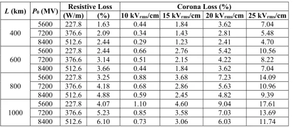
Table 5-5:. Resistive and Corona Loss Percentage of 1000 kV AC Single-circuit Three-phase Transmission Lines under glaze condition ... 80
Table 5-6: Comparison of Corona Onset Voltages (V0) after 40 Minutes of Rime Accretion. ... 83
Table 5-7: Comparison of Corona Onset Voltages (V0) after 40 Minutes of Glaze Accretion. ... 83
Table 5-8: Calculated Values of Surface Irregularity (m) after 40 Minutes of Rime Accretion (-15 ℃). ... 86
Table 5-9: Calculated Values of Surface Irregularity (m) after 40 Minutes of Glaze Accretion (-8 ℃). ... 86
Table 5-10: Comparison of Measured Guc under Different Icing Conditions. ... 88
Table 5-11: Icicle length after 40 minutes of glaze ice accretion when the wind velocity is 2 m/s at different conductor surface electric fields. ... 92
Table 5-12: Harmonic components to the corresponding fundamental (%) under rime and glaze ice conditions. ... 97
Table 5-13: THDV and THDC at different conductor surface electric field strengths under different weather conditions. ... 98
Table 6-1: Simulation Parameters of Rime Accretion ... 126
Table 6-2: Statistics for the meshes employed ... 126
Table 6-3: The Calculated Overall Collision Efficiency of Particles at Different Conductor Surface Electric Field Strengths with a Wind Velocity of 2 m/s. ... 129
LIST OF FIGURES
Figure 2-1: Glaze on a conductor in the experiment ... 12
Figure 2-2: Soft rime on a conductor in the experiment ... 12
Figure 2-3: Hard rime on a conductor in the experiment ... 13
Figure 2-4: Surface hoar plates on pine needle tips ... 15
Figure 2-5: Major AC systems in chronological order of their installations. ... 17
Figure 2-6: Schematic diagram of a corona cage. ... 23
Figure 2-7: An indoor corona cage at Tsinghua University. ... 24
Figure 2-8: Outdoor corona cage at Wuhan Bureau of China Electric Power Research Institute. ... 25
Figure 2-9: Outdoor corona cage at UHV DC Testing Site in Beijing. ... 26
Figure 2-10: Outdoor test line at UHV AC test base of China Electric Power Research Institute. ... 27
Figure 3-1: Climate room with corona cage ... 33
Figure 3-2: Spraying system ... 34
Figure 3-3: Schematic diagram of spray nozzle for ice accretion. ... 34
Figure 3-4: Schematic diagram of test circuit. ... 35
Figure 3-5: Laboratory corona cage. ... 36
Figure 3-6: The simulated conductor surface electric field distribution along the conductor. ... 37
Figure 3-7: Data acquisition board NI PCI-6251 ... 39
Figure 3-8: OMEGA HHF710 ... 40
Figure 3-9: Balance APX-1502 ... 40
Figure 3-10: Balance APX-1502 ... 41
Figure 3-11: Stabilization process of two different methods ... 43
Figure 4-1: Accreted rimes at different electric fields. ... 48
Figure 4-2: Icicles formed at different electric fields. ... 49
Figure 4-3: Weight of rime under various energized conditions. ... 50
Figure 4-4: Weight of glaze ice under various energized conditions. ... 51
Figure 4-5: Cross-section of a pendant drop. ... 58
Figure 4-6: Diameter measurement of icicles. ... 62
Figure 4-7: Icicle lengths at different electric fields and wind velocities when PR=15 mm/h. ... 63
Figure 4-8: Convective heat transfer coefficient vs. wind velocity. ... 64
Figure 4-9: Icicle deviation angle at different electric fields. ... 65
Figure 4-10: Diagram of icicles and force analysis of the icicle tip. ... 66
Figure 4-11: Angles between adjacent icicles at different electric fields ... 66
Figure 5-1: Appearance of accreted ice and its corona discharge. ... 71
Figure 5-2: The equivalent circuit representing the corona process from the conductor-cage configuration. .. 71
Figure 5-3: Corona losses at different electric field strengths during rime accretion with wind velocity of 2 m/s and conductivity of 50 μS/cm. ... 72
Figure 5-4: Corona losses at different electric field strengths during rime accretion with wind velocity of 3 m/s and conductivity of 50 μS/cm. ... 72
Figure 5-5: Corona losses at different electric field strengths during glaze accretion with wind velocity of 2 m/s and conductivity of 50 and 200 μS/cm (A and B stand for conductivities of 50 and 200 μS/cm). ... 75
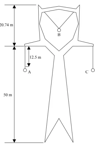
Figure 5-6: The schematic diagram of the test line tower ... 77
Figure 5-7: Corona losses vs. voltage at different electric field strengths for rime accretion. ... 81
Figure 5-8: Corona losses vs. voltage at different electric field strengths for glaze accretion. ... 82
Figure 5-9: Corona losses – quadratic analysis. ... 82
Figure 5-10: Measured Guc during rime accretion process at different conductor surface electric field strengths. ... 86
Figure 5-11: Measured Guc during glaze ice accretion process at different conductor surface electric field strengths. ... 87
Figure 5-12: Fundamental components of applied voltage and the induced corona current. ... 89
Figure 5-13: Measured Cuc during rime accretion at different conductor surface electric field strengths. ... 90
Figure 5-14: Measured Cuc during glaze ice accretion at different conductor surface electric field strengths. . 91
Figure 5-15: Radius of equivalent coronal conductor at different conductor surface electric field strengths. .. 92
Figure 5-16: Voltage and current harmonic spectrums and their composite waveforms after 40 minutes of rime accretion with V = 55.1 kV. ... 95
Figure 5-17: Voltage and current harmonic spectrums and their composite waveforms after 40 minutes of
glaze ice accretion with V = 137.7 kV. ... 96
Figure 5-18: Ratio of THDC and THDV at different conductor surface electric strengths under different weather conditions. ... 99
Figure 5-19: Power factors during the glaze ice accretion process with an applied voltage of 137.7 kV ... 100
Figure 5-20: Power factors during the rime accretion process with applied voltage of 137.7 kV. ... 101
Figure 5-21: Harmonic corona loss in percentage of total corona loss of the glaze ice accretion with an applied voltage of 137.7 kV. ... 101
Figure 5-22: The power factor vs. time and voltage under rime. ... 106
Figure 5-23: The power factor vs. time and voltage under glaze condition. ... 109
Figure 6-1: Model structure ... 115
Figure 6-2: Flow diagram of simulation ... 115
Figure 6-3: Reduced computational zone ... 116
Figure 6-4: Grazing trajectories of water droplets ... 122
Figure 6-5: Definition of local collision efficiency ... 123
Figure 6-6: Growth of ice surface ... 125
Figure 6-7: Mesh of the domain in the initial stage. ... 127
Figure 6-8: Airflow past the cylinder when the wind velocity is 2 m/s. ... 128
Figure 6-9: Water droplets captured and their impaction velocities (the water droplet is not to scale). ... 129
Figure 6-10: The definition of Y and L. ... 130
Figure 6-11: The relationship between Y and L. ... 130
Figure 6-12: The local collision efficiency curves along the conductor surface when the wind velocity is 2 m/s, droplet diameter is 59 μm, and conductor surface electric field is -25 kV/cm. ... 131
Figure 6-13: Rime accreted after 40 minutes of accretion with electric filed E = -5 kV/cm ... 132
Figure 6-14: Ice sample removed from conductor ... 132
Figure 6-15: Comparison of ice shape, V = 2 m/s, and D = 38 μm, LWC = 2.1 g/m3 ... 134
Figure 6-16: Comparison of ice weight ... 135
Figure 6-17: E = -20 kV/cm, V = 4 m/s, and D = 38 μm, LWC = 1.05 g/m3... 135
Figure 6-18: Rime accreted after 40 minutes of accretion, E = -10 kV/cm, V = 2 m/s, and ... 136
ACKNOWLEDGMENTS
This work was carried out within the framework of the NSERC/Hydro-UQAC Industrial Chair on Atmospheric Icing of Power Network Equipment (CIGELE), the Canada Research Chair on Atmospheric Icing Engineering of Power Networks (INGIVRE) at Université du Québec à Chicoutimi (UQAC), and also in collaboration with the National Basic Research Program of China (973 Program: 2009CB724501/502/503).
I would like to express my deepest gratitude and admiration to my supervisor, Prof. Masoud Farzaneh, for granting me the invaluable chance to pursue my Ph. D study, his supervision, encouragement, support, and especially patience during the entire research. Without his patience and continuous help, this research would not have been possible.
I want to deliver my sincere gratitude and respect to my co-supervisor Prof. Xingliang Jiang, for not only his guidance, valuable advices, but also human qualities and supports.
Special thanks go to Prof. William. A. Chisholm from Kinectrics for his insightful comments and constructive suggestions during my doctoral examination process. Many thanks also go to Prof. Issouf Fofana, Prof. Gelareh Momen, and Prof. Shamsodin Taheri for their constructive criticism which contributed to improve the quality of this thesis.
I would like to extend my thanks to Claude Damours, Pierre Camirand, and Xavier Bouchard at CIGELE Laboratory for their technical support and to Denis Masson for his help with administrative tasks.
Finally, I would like to take this opportunity to thank my son, Mingzhe Yin, for his unconditional love during these years.
CHAPTER 1
INTRODUCTION
CHAPITRE 1 INTRODUCTION
1.1 Definition of the problem
The study of ice and snow accretion on structures is of great interest to engineers and scientists. In cold regions, atmospheric icing affects a wide variety of man-made structures in many countries [1][2], including overhead transmission lines, telecommunication towers, and wind turbines. These structures are installed across mountains, making ice events more likely to happen.
Wet snow accretion, as reported by Colbeck et al [3], is known to be particularly troublesome since a large mass accumulation can occur in only a few hours. Snow accretion on overhead transmission lines and wires may thus be considered as a serious problem posing tremendous threats to existing power installations. As extra-high voltage (EHV, in the range of 230 kV and 800 kV [4]) and ultra-high voltage (UHV, referring to above ± 800 kV for DC and 1000 kV for AC [5]) power transmission lines are running not far away from their disruptive critical voltages, in unfavorable icing conditions, it can be expected that these lines will operate for considerable periods in the presence of corona discharges [6]. The existence of corona discharge can cause audible noise (AN), radio frequency interference (RFI), and corona loss (CL) which should be minimized for economic reasons [7][8]. In addition to corona losses induced by ice accretion, subsequent ice shedding tends to cause power outages and severe damage to power network structures, thereby leading to many serviceability, safety, and mechanical reliability issues. Many countries such as Canada, the United States, the United Kingdom, France, Germany, Norway, Iceland, and Japan experience wet snowfalls which affect the related overhead transmission networks.
The damage caused by a single wet snowstorm can necessitate the expenditure of sums on the order of 100 million dollars. Past records show that the occurrence of wet snow accretion is relatively more common and may be equally as catastrophic in Japan, Canada, United Kingdom, Iceland, Russia
and China every year. Two records of these ice storms were most destructive. One is the North American Ice Storm of 1998 which was a massive combination of five smaller successive ice storms which combined to strike a relatively narrow swath of land from eastern Ontario to southern Quebec to Nova Scotia in Canada, and bordering areas from northern New York to central Maine in the United States, in January 1998 [9]. It caused massive damage to trees and electrical infrastructure all over the area, leading to widespread long-term power outages. As a result, over 4 million people in Ontario, Quebec and New Brunswick were deprived of power. More than 1,000 power transmission towers were destroyed and 30,000 utility poles fell for an estimated loss of $5.4 billion dollars [6]. The other one is the 2008 Chinese Ice Storm, which struck the most populated and economically developed region of China and was even more damaging than the 1998 North American Ice Storm. There were 13 provincial grids (approximately 43% of the total power at the provincial level) affected, and the users of nearly 570 counties were subject to power outages. According to statistics released by the Ministry of Civil Affairs of China, the ice storm led to 107 deaths and the direct economic losses alone were about $22 billion and the indirect losses could be even greater [10].
Corona loss is one of the most important issues associated with EHV and UHV power transmission systems [11-13]. This problem is of great significance in Canada [14], especially in Quebec, Newfoundland, etc. which have as many as 80 snowy days a year with an annual average snowfall more than 300 centimeters based on weather data collected from 1981 to 2010. The influence of ice accretion on corona discharge has been investigated since the beginning of high voltage transmission. Initially, losses of energy were of primary interest and, as early as 1912, F. W. Peek stated that the effect of snow was greater than that of any other weather condition [15]. After that, many attempts were made to find some quantitative relations atmospheric conditions and corona losses. However, most of them were carried out on test lines and operating lines, with the atmospheric condition varying. In the present study, the corona investigation was performed in a climate room, with all ambient parameters constant during the tests.
Presently, there are mainly three methods to investigate the CL on the conductor, namely the corona cage [16-18], outdoor test lines [11, 19-20] and operating lines [21-24]. However, in the last two cases, the losses measured are composed of several components such as insulator loss, CL from conductor surface and some loss in the earth. It is very difficult to separate these losses from one another.
Ice accumulation coupled with the wind-on-ice load may lead to the failure of structures and their function. Typical outcomes are endangering for human life in aircraft or marine icing incidents, and in the loss of industrial resources due to faults on an overhead transmission line grid system. Regarding the latter, structural damage can be extensive, running up to millions of dollars and, moreover, the effects of power outages are known to be severe in both human and industrial terms. Thus, much progress has been made in understanding the physical process involved during ice accretion on structures. Three main methods of investigation are the following ones [2]:
1) Continuous field measurement of ice load and wind-on-ice load, allied with the simultaneous measurements of meteorological variables;
2) Simulations using icing wind tunnels for un-energized icing or corona cage for energized icing;
3) Construction of mathematical/computational icing models.
From the viewpoint of engineering design, the generation of an ice load database, with corresponding historical weather database, is of major importance. Furthermore, such databases are essential in the validation of experimental and theoretical simulations of the icing process. Obviously, this approach involves high cost in the installation of measurement sites, for a geographical location, and in the manning of such sites by icing engineers and meteorologists. The study of ice simulation employing an icing wind tunnel or corona cage has the advantage that the effects of changes in the flow and thermal conditions on the accretion process can be readily assessed and analyzed. A disadvantage
of this method is that due to the many physical and meteorological variables and the flow and thermal parameters controlling an accretion process, it is difficult to achieve a one-to-one correspondence between the icing wind tunnel/corona cage and field conditions. The third method involving theoretical models, based on the known physics of the accretion process, has obvious advantages especially when implemented in the form of mathematical models. In this project, an attempt will be made to develop the theory of ice accretion in a systematic way, based on principles of fluid mechanics, mass transfer, and electric field using mathematical and numerical techniques.
1.2 Research objectives
The main goal of this research work is to investigate the effect of electric field strength and corona discharge on ice accreted on high-voltage conductor. To achieve this aim, the research is approached by two methods, experiments and simulations. The specific objectives of this research are listed as follows.
1.2.1 Experiments
Investigating the effect of electric field strength on ice formation. Due to the Joule heat, the ice appearance will be affected by the existence of electric field. Moreover, as ice load is an important factor when designing the power transmission line, ice weight, icicle spacing, icicle length, and angle between adjacent icicles should also be investigated.
Investigating the effect of electric field strength on corona characteristics under icing conditions. To get detailed information about the influence of electric field on corona characteristics, the corona loss, corona onset voltage, harmonic distortion, leakage conductance, and capacitance of an energized conductor under icing conditions should be studied.
1.2.2 Simulations
Developing an applicable time-dependent numerical ice model for simulating the rime accretion process on fixed conductors under energized conditions. Many simulation models of ice accretion have been developed. However, all of these models deal with un-energized conditions. In reality, the transmission lines exposed to icing are subjected to electric field. Therefore, to investigate the ice accretion on transmission lines, it is appropriate to improve the existing numerical model by considering the influence of electric field.
Establishing a numerical technique for model application. Icing is a very complex phenomenon for which an analytical solution is not available. Also, the governing equations for modeling its behavior are non-linear and not easy to solve. Therefore, developing a technique which can deal with the non-linear equations is crucial.
Validating the simulation results with the experimental data. A good measurement of the reliability of the model would be a good agreement of its predicted results with the experimental data. For this reason, the developed model and the numerical results obtained from it should be validated by experimental data.
1.3 Methodology
To achieve the above objectives, experiments and simulations were carried out at CIGELE laboratories, University of Quebec in Chicoutimi (UQAC). The methodologies for them are described as follows:
As icing is a very complex process and its formation can be greatly influenced by the variation of environmental parameters, it is very important that the weather parameters are kept constant during the whole ice accretion process. Thus, the experiments were performed in a delicate climate room which is designed especially for atmospheric research. To apply an electric field on the conductor, a corona cage was adopted. One major advantage of using a corona cage is that the close distance between the tested conductor and grounded meshed cylinder can replicate the surface electric field of a practical transmission line at a much lower applied voltage. With careful control, the measurements carried out in the CIGELE climate room were found to be repeatable.
2) Simulations
For simplicity, simulation will be carried out on a smooth conductor. Numerical modeling of atmospheric ice accretion is based on the following steps:
Airflow computation. As the wind velocity investigated in this paper is less than Mach 0.3, the airflow can be assumed to be incompressible.
Droplet trajectory calculation. The trajectory of water droplets will be modeled based on the balance between aerodynamic force, gravity, buoyancy force and dielectrophoretic force.
Local collision efficiency. After the water droplet trajectory is calculated, the local collision efficiency can be obtained.
Updating the ice layer. With the local collision efficiency known, the mass accreted in each section on the surface of the ice conductor can be computed. In each iteration, the ice layer is updated.
1.4 Statement of the originality of the thesis
To the best of our knowledge, no systematic study has been done on the influence of electric field strength on corona discharge of ice accreted conductor. Also, previous ice accretion simulations were only focused on the conductor without high-voltage applied, in which the corona electric force were not considered. The main original contributions of this PhD project are summarized as follows:
1) The effect of electric field strength on ice formation was investigated.
2) A detailed analysis of electric field strength on corona characteristics was carried out.
3) A time-dependent numerical ice accretion simulation including the effect of electric field strength was developed.
1.5 Thesis outline
The structure of this dissertation is as follows:
Chapter 1 introduces the problem of ice accretion on power network, the necessity, research objectives, methodology, and originality of the present research.
Chapter 2 reviews the literature related to corona loss measurement. Moreover, a survey of numerical modelling for predicting the ice accretion is introduced.
Chapter 3 describes the experimental facilities and the test procedures for performing the experiments in the laboratory.
Chapter 4 presents the influence of electric field strength on ice formation. Laboratory results show that electric field strength has significant influence on ice appearance, ice weight, icicle spacing, icicle length, and also angle between adjacent icicles.
Chapter 5 focuses on the dynamic corona characteristics of an energized conductor during the ice accretion process.
Chapter 6 deals with the rime accretion simulation and its experimental validation in laboratory.
Chapter 7 provides general conclusions derived from the results and discussion covered in the previous chapters. Several recommendations for the future work are also presented.
CHAPTER 2
CHAPITRE 2 REVIEW OF LITERATURE
2.1 Types of atmospheric icing accretion
Atmospheric icing is a generic term for all types of accretion of frozen water substance [1] [25]. Various processes where water in various forms in the atmosphere freezes and adheres to objects exposed to the air. In general, the atmospheric icing accretion can be classified in the following types.
(1) Precipitation icing
(2) In-cloud icing
(3) Hoar frost
2.1.1 Precipitation icing
Precipitation icing occurs in several forms such as freezing rain (glaze or rime), wet snow and dry snow depending on how the precipitation is influenced by variations in temperature near the ground and up to a few hundred meters above ground. Such icing is experienced any place where precipitation, in combination with freezing temperatures, occurs. Different types of precipitation icing are described below:
Glaze: Glaze has a density higher than 900 kg/m3 [26]. Glaze grows in a clear, smooth structure with no air bubbles, as shown in Figure 2-1. It is usually formed from freezing precipitation, rain or drizzle, or from clouds with large liquid water content and large drop size. The freezing rate of droplets is less than the impingement rate, which causes part of the drop to splash or flow around the conductor
before freezing. While glaze contains no air bubbles as such, in strong wind situations it grows in irregular shapes incorporating pockets of air.
Figure 2-1: Glaze on a conductor in the experiment
Figure 2-2: Soft rime on a conductor in the experiment
Rime: Rime has a density of 300 - 900 kg/m3[27]. It is usually classified as soft rime or hard rime:
Soft rime has a density of less than 600 kg/m3. Figure 2-2 shows soft rime on a conductor in the experiments. It is a white ice deposition that forms when the water droplets in light freezing fog or mist freeze to the outer surfaces of objects, with calm or light wind. The fog freezes usually to the windward
side of tree branches, wires, or any other solid objects. Soft rime is similar in appearance to hoar frost; but whereas rime is formed by vapor first condensing to liquid droplets (of fog, mist or cloud) and then attaching to a surface, hoar frost is formed by direct deposition from water vapor to solid ice. Soft rime grows in a triangular or pennant shape pointed into the wind. The granular structure results from the rate of freezing of individual drops, each drop freezing completely before another one impinges on the surface. They are fragile and can be easily shaken off objects. Factors that favor soft rime are small drop size, slow accretion of liquid water, high degree of super-cooling, and fast dissipation of latent heat of fusion.
Hard rime has a density ranging from 600 to 900 kg/m3 and tends to grow in a layered structure with clear ice mixed with ice containing air bubbles [28]. In this case the freezing rate of the droplets is equal to the impingement rate. It is a white ice that forms when the water droplets in fog freeze to the outer surfaces of objects. It is often seen on trees at mountains and ridges in winter, when low hanging clouds cause freezing fog. This fog freezes to the windward (wind-facing) side of tree branches, buildings, or any other solid objects, usually with high wind velocities and air temperatures between -2 and -8 °C (28.4 and 17.6 °F). Hard rime formations are difficult to shake off; they have a comb-like appearance, unlike soft rime, which looks feathery or spiky, or clear ice, which looks homogeneous and transparent. Figure 2-3 shows hard rime accreted on a conductor.
Both rime types are less dense than glaze and cling less tenaciously, therefore damage due to rime is generally minor compared to glaze.
Wet snow: Wet snow has a density of 300 - 800 kg/m3. It is usually defined as snow which falls at temperatures equal to or above -5 . Under these conditions, the snow is sticky enough to adhere to surfaces easily and accumulate rapidly. Wet snow tends to build on tops and windward surfaces of structures and in cylindrical layers around conductors [1]. At temperatures below about -2 , snow particles are usually too dry to adhere to surfaces in appreciable quantities. If the temperature falls below 0 after the accretion of wet snow, the accumulation freezes into a dense hard layer with strong adhesion. Transmission line problems have occurred due to wet snow events.
Dry snow: Dry snow accretes at subfreezing temperatures [29-30]. This type of accretion appears only when wind speed is very low i.e. below 2 m/s. The density of dry snow is, in general, very low, not exceeding 100 kg/m3. Hence the accreted masses are, in most cases, much lower than the loads the power lines are designed for.
2.1.2 In-cloud icing
In-cloud icing occurs only within clouds consisting of super-cooled droplets, which are droplets that remain liquid at a temperature below 0 [31]. It is a process by which super-cooled water droplets in a cloud or fog freeze immediately upon impact on objects in the airflow, i.e. overhead lines in mountains above the cloud base. For the structures situated at mountain summits, exposure to super-cooled clouds or fog usually results in soft rime (300 - 600 kg/m3), however, precipitations resulting in hard rime (600 - 900 kg/m3) also occur and are most frequent in early winter. Sometimes very large in-cloud icing occurs on overhead lines.
2.1.3 Hoar frost
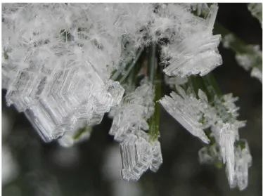
Hoar frost: Hoar frost has a density of less than 300 kg/m3. Figure 2-4 shows hoar frost that grows on pine needle tips [32]. Hoar frost is generally a deposit of interlocking ice crystals formed by direct sublimation of water vapor in the air onto objects. It forms when air with a dew point below freezing is brought to saturation by cooling. Hoar frost is featherlike in appearance and builds occasionally to large diameters with very little weight. Normally, hoar frost does not constitute a significant loading problem, however, it is a very good collector of super-cooled fog or cloud droplets and at subfreezing temperatures with light winds, fog conditions gradually become soft rime of significant volume and weight. Furthermore, its presence on the overhead transmission lines can still cause very significant energy losses due to corona discharge [33].
Figure 2-4: Surface hoar plates on pine needle tips
Of all the above-mentioned types of ice accretion, rime and glaze are most dangerous to the power system. Therefore, the present paper deals only with rime and glaze ice accretion.
2.2 Corona loss
2.2.1 Electric power system
Modern electric power systems are the result of over a hundred years of development in which the technical and economic feasibility of transmitting large blocks of power over long distances played an important role [34]. The first public power station was put into service in 1882 in London (Holborn). Soon a number of other public supplies for electricity followed in other developed countries. By 1890, the art in the development of an AC generator and transformer had been perfected to the point when AC supply was becoming common, displacing the earlier DC system. The first major AC power station was commissioned in 1890 at Deptford, supplying power to central London over a distance of 28 miles at 10 kV. Prior to this, electric power was generated and used locally in either a laboratory or industrial setting. Thomos Edison is generally regarded as the one sowing the seeds of modern power system by conceiving the Pearl Street station in New York [35], in which the generator was used to supply a number of his newly-invented incandescent lamps.
An important problem facing the early power systems was the efficiency of power distribution using metallic wires, usually copper, over distances of even a few kilometers [36]. In fact, the occurrence of heavy power losses in the resistance of the distribution wires at low voltages made these systems uneconomical, as the need for larger quantities of power and longer distances increased. For given quantity of power, the use of a higher transmission voltage results in a lower current in the conductors and therefore in lower power losses and higher efficiency.
High voltage transmission gave rise, not only the economic feasibility of transmitting large blocks of power over long distances, but also resulted in the development of large power networks in which geographically separated generating stations and load centers are interconnected [37]. Improved economy and reliability were the main factors pushing the evolution of large interconnected power system.
The rapidly increasing transmission voltage level in recent decades is a result of the growing demand for electrical energy, coupled with the development of large hydroelectric power stations at sites far remote from centres of industrial activity and the need to transmit the energy over long distances to the centres. Figure 2-5 lists some of the major AC transmission systems in chronological order of their installations [34]. 1 1890 10 kV Deptford 2 1907 50 kV Stadtwerke München 3 1912 110 kV Lauchhammer − Riesa 4 1926 220 kV N. Pennsylvania 5 1936 287 kV Boulder Dam 6 1952 380 kV Harspränget − Hallsberg 7 1959 525 kV USSR 8 1965 735 kV Manicouagan – Montreal 9 1989 1200 kV Soviet Union
10 2003 500 kV Three Gorges (China)
11 2009 1000 kV Jindongnan-Nanyang-Jingmen (China) Figure 2-5: Major AC systems in chronological order of their installations.
Corona losses upon transmission lines may reach values worthy of serious consideration of the designing and operating electrical engineer at or above potentials of 100 kV between wires [38], depending upon the size and spacing of wires, the weather conditions and the elevation of the line above sea level. Power loss due to corona atmospheric icing is very complicated and occurs in a variety of forms as a result of the interplay of numerous physical processes.
2.2.2 Conductor corona onset gradient
Atmospheric air is probably the most important insulating material used on high voltage transmission lines [39-40]. At sufficient high levels of conductor surface electric fields, complex ionization processes take place in the air surrounding high voltage transmission line conductors, resulting in discharge phenomena known as corona.
Onset voltage is defined as the initiation of a self-sustaining discharge near the conductor, and occurs when the conductor surface electric field strength exceeds a critical value [41-42]. The corona onset gradient is a function of the conductor diameter and its surface condition as well as of the ambient temperature and pressure [39] [43-47]. The corona onset gradient of cylindrical conductors has been studied experimental and empirical formulas have been developed for alternating and direct applied voltages. In general, the corona onset gradient Ec of a cylindrical conductor is given as [48]
0 (1 ) (2.1) c c K r E mE
where E0 and K are empirical constants depending on the nature of the applied voltage, δ is the relative air density factor. These values for AC, according to Peek, are E0 = 21.1 kVrms/cm and K = 0.308 for the case of concentric cylindrical geometry.
The empirical formula described above was derived from laboratory experiments on smooth conductors with diameters much smaller than those used on practical transmission lines. The diameter of the out cylinder was also small in these laboratory studies. However, it was found that this formula can be extrapolated to practical conductor sizes.
Conductor surface irregularity factor m is equal to 1 for ideally smooth and clean conductors [49]. Even microscopic imperfections on the conductor surface tend to reduce the value of m below 1 [50]. Practical transmission line conductors are generally of stranded construction, comprised of several layers of small diameter cylindrical strands. Experimental results have shown that the value of m may
vary between 0.75 and 0.85 for stranded conductors, depending on the ratio of strand to conductor diameter. Under the rain and icing conditions, the value of m may be reduced by the water drops, icing treeing, and icicles.
2.2.3 Conductor corona loss predication
The corona performance of a transmission line, as defined by the resulting effects such as corona loss (CL), radio interference (RI), and Audible noise (AN) [6], depends mainly on two sets of factors: a) line design; b) ambient weather conditions [39-40]. The line design factors of interest are the type and dimensions of the conductor, phase spacing in the case of AC lines and pole spacing for DC lines, and the height above ground of the conductors. The most important factor that influences the generation of corona, however, is the electric field distribution in the vicinity of the conductor surface [38]. The second set of factors, namely the ambient weather conditions, influence the corona performance in two ways: first, the temperature, pressure, and relative humidity of the ambient air affect the basic ionization processes involved in corona discharge; and second, any precipitation such as rain or snow deposited on the conductor surface distorts the electric field in the vicinity.
The design of transmission lines for acceptable corona performance generally results in the conductors or conductor bundles operating at conductor surface electric field strengths that are close to their corona onset gradient under normal fair weather conditions [51-52]. As a result of normal design considerations, the occurrence of corona discharges, at the nominal operating voltage and in fair weather, are limited. Under foul weather conditions, such as rain or icing, there is an intensive corona discharge, nearly uniform distributed, along the conductor [6].
Corona losses under heavy rain or icing conditions of practical transmission lines may reach the same order of magnitude as the I2R loss at full load on the line. In fair weather, corona loss are generally two or three orders of magnitude lower than those under heavy rain or glaze ice conditions. Under other weather conditions, such as fog, light rain, or snow, corona losses are somewhat lower than
those under heavy rain or glaze ice conditions, but much higher compared to fair weather losses [16] [15][22-23][53-54]. From a practical point of view, therefore, the corona loss under fair weather are negligible.
Form the point of view of transmission line design, the most useful corona loss parameter is the mean annual corona Pma, which can be defined as [55]
1 1 i i (2.2) ma a n PT T i P
where i ranges from 1 to N is the different weather categories for which the corona loss Pi is known, Ti is the time duration in hours of the ith weather category in a year, and Ta = 8760, is the total number of hours in a year.
To determine pma for a transmission line located in a given region, two sets of information should be given:
1) The generated corona loss for the actual conductor used, as a function of the conductor surface electric field strength under different categories of weather conditions.
2) The annual weather patterns occurring in the region where the line is located.
The first can be obtained through tests on the conductor or from empirical formulas and the second may be got from the nearby meteorological station.
Corona loss formulae were initiated by F.W. Peek Jr. in 1912 derived empirically from most difficult and painstaking experimental work [54]. Since then, a number of formulae have been derived by others, both from experiments and theoretical analysis [47] [56-58].
In 1961, Nigol put forward a corona loss equation for single and bundled conductors. The basic form is express as [20] 2 2 0 2
ln
(2.3) e e E E P Kfr E where P is the corona loss per conductor, in kW/mile, K is a dimensionless conditional constant for the given weather and conductor surface conditions, f is the frequency, r is the radius of the conductor, Ee is the effective surface electric field strength, in kVrms/cm, E0 is the critical surface electric field strength for given weather and conductor surface conditions, in kVrms/cm, and Δρ is the angular portion of conductor surface in corona, in radians. For a single conductor at normal phase spacings, the value Ee is almost constant over the conductor surface and is equal to the maximum surface electric field strength Em. Because of this, corona on single conductor is assumed to cover the entire surface, and the angle Δρ is equal to 2π. Therefore, the above equation for single conductor becomes
2 2 0 (2.4)
ln
e e E E P Kfr E For bundled conductors with non-uniform surface electric field strength, both the effective surface electric field strength and the portion of conductor surface in corona must be evaluated before the corona loss can be calculated.
Extending over the yeas 1967 and 1968, Clade carried out more than 20, 000 measurements using a corona cage [53]. The measured values were reduced to normalized values and then been plotted into a universal chart. After that, the corona loss on UHV lines under rain can be predicated with conductor surface state coefficients.
2.3 Measurement methods for corona performance
Theoretical considerations are necessary to provide a basic understanding of corona phenomena occurring on transmission line conductors and of the resulting corona effects [38]. However, the very complex nature of corona phenomena, combined with the large number of factors influencing corona
effects, making experimental studies essential for evaluating the corona performance of transmission lines. Good experimental data is a basic requirement for the development of accurate empirical and semi-empirical methods of calculation. The choice of instrumentation and measurement techniques, for the various parameters defining corona performance of a transmission line, plays an important role in planning and carrying out the experimental studies [38][59]. Different test methods, ranging from test in laboratory corona cage to measurements on operating transmission lines, may be used for obtaining the necessary data. In the early studies, it is economically impractical to construct long test lines and replace conductors of varying dimensions frequently for corona tests. Usually, the UHV test bases and similar research institutes obtain data from corona tests on short test lines and then convert them to equivalent data for long three-phase lines.
The main objective of experimental corona studies on conductors are: 1) to understand the physical mechanisms involved in corona discharge as well as the resulting corona effects, and 2) to generate experimental data that can be used to develop prediction methods for the corona performance of transmission lines. The principal corona test methods used and the aspects of corona performance that can be studied by each of them are described as follows
2.3.1 Laboratory corona cage
To understand the physics of corona discharges, laboratory studies have been carried out using a variety of electrode geometries, such as point-plane, sphere-plane, concentric-spherical etc. [7][40][61-65]. Most of the laboratory studies of corona on cylindrical conductors have been made, however, using what is commonly known as a “corona cage” configuration. In fact, the empirical formulas for determining corona onset on smooth and stranded conductors were obtained mainly from corona cage tests [48].
A corona cage usually has two layers as shown in Figure 2-6. The out layer is the shielding cage and the inner layer is used for the measurement of corona with a round or square cross-section. During
the test, test conductors are usually placed at the center of a corona cage. Because the conductors are placed near the corona cage, surface fields with strength comparable with those on an UHV transmission line conductor can be produced when a lower test voltage is applied to the conductor [41]. In general, high voltage is applied to the conductor, with the inner cage maintained at zero potential by connecting it to ground through a small measuring impedance. In special cases involving measurement of fast-rising corona current pulses, the situation may be reversed by applying high voltage to the cage and keeping the conductor at ground potential.
Figure 2-6: Schematic diagram of a corona cage.
For a corona cage of finite length, the electric field distribution in the longitudinal direction is uniform over the central section of the conductor and becomes non-uniform at both ends. By adding guard sections, the central section of the corona cage can be selected to obtain a fairly uniform electric field distribution along the length of the conductor. The central section of the corona cage is then used for the corona measurements by connecting it to ground through appropriate measuring impedance, while the two guard sections are connected directly to ground.
The main advantage of the corona cage test setup is that the conductor surface electric field distribution can be determined quickly and accurately from a knowledge of the voltage applied and the dimension of the test configuration. For round cross-section corona cage, the uniformly distributed conductor surface gradient Ec in kV/cm can be calculated quite accurately as [43]
(2.5) ln( / ) app surface c c U E r R r
where Uapp (kV) is the voltage applied to the conductor, rc is the conductor radius in cm, and R is the radius of the cage in cm. Different values of the conductor surface electric field strengths are obtained by varying the voltage applied.
Figure 2-7: An indoor corona cage at Tsinghua University.
The main criterion for the design of a corona cage test setup, for use either in a laboratory or outdoors, is to have an adequate margin between the breakdown and corona onset voltages. For the conductor to be tested, the cage diameter should be small enough to obtain corona onset at a sufficiently low voltage [66]. At the mean time, the air gap between the conductor and the cage should be large enough so that the breakdown voltage is higher than the corona onset voltage. Figure 2-7 shows an indoor corona cage at Tsinghua University [67].
2.3.2 Outdoor corona cage
To test conductor configuration generally used on transmission lines, the corona cages have to be much larger than those of laboratory cages, which is the main reason why they are built outdoors. Outdoor corona cages also permit experimental data to be obtained under some natural weather conditions.
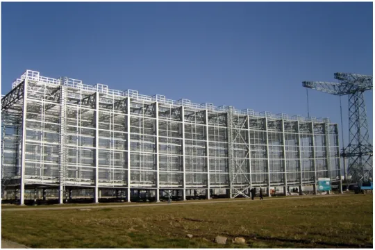
Figure 2-8: Outdoor corona cage at Wuhan Bureau of China Electric Power Research Institute.
An outdoor test corona cage arrangement consists essentially of conductor configurations placed at the center of a wire-mesh enclosure of either circular or square cross section [17]. The square cross section is usually preferred because of difficulties in fabricating cylindrical cage enclosures of large diameter. In some cases, the cage enclosure may simply consist of two vertical fences, with the ground acting as the lower panel and the top left open. As in the case of laboratory cages, outdoor corona cages are often built with an insulated central measuring section and two guard end sections. Outdoor cages have frequently been used mainly to determine the corona performance under heavy rain conditions, by equipping them with means for producing artificial rain, or at different altitudes [68-70]. Figure 2-8 shows an outdoor corona cage developed by Wuhan bureau of China Electric Power Research
Institute. It has the following features: (a) it incorporates a hybrid electronic current transformer that allows the safe and reliable measurement of the current through conductors in the corona cage; (b) by using an outdoor high-accuracy capacitive voltage divider, it is possible to accurately measure the voltage; and (c) the voltage signals are transmitted through coaxial cable and the current signals are transmitted through optical fiber. Based on the accurate voltage and current signals extracted, the system can measure the corona loss of conductors with the aid of the digital signal processing and virtual instrumentation technologies.
Figure 2-9: Outdoor corona cage at UHV DC Testing Site in Beijing.
In regions where snow accumulation on the ground in winter may be a problem. It is necessary to place the cage enclosure at a certain height above ground. If the cage length is more than about ten meters, the cage enclosure is made to follow the catenary shape of the conductor, so that the conductor is located at the center of the cage all along its length. Figure 2-9 shows the outdoor corona cage at UHV DC Testing Site in Beijing with a catenary shape, used for single pole and dual pole tests with maximum testing voltage up to ±1200kV [71]. It is the biggest outdoor cage so far, with a dimension of 70 m× 22m × 15 m (L×W×H).
2.3.3 Outdoor test lines
Although outdoor test cages provide a comparatively rapid and inexpensive means for evaluating the corona performance of conductor configurations, mainly in heavy rain, they cannot be used to obtain the all-weather statistical corona performance. Such statistical data in fair weather as well as foul weather can be obtained only from outdoor lines.
Figure 2-10: Outdoor test line at UHV AC test base of China Electric Power Research Institute.
Outdoor test lines are essentially short sections of full-scale transmission lines [19]. For AC corona studies, either single-phase or three-phase test lines may be used. Three phase test lines accurately reproduce the electric field conditions of normal transmission lines [60]. For this reason, most of the corona studies for the purpose of providing design data for transmission lines at new higher voltage level have been carried out on three-phase test lines [11][13][38][60]. In 1963, Laforest presented the corona loss and radio noise investigation from a EHV project at a heavily instrumented lest line with 4.3 miles of under fair and foul weather. Insulator loss and the dependence of corona loss on load current were also discussed [72]. Figure 2-10 shows an outdoor test line at UHV AC test base of China Electric Power Research Institute, used for AC corona studies with 8 towers and a length of 1084 m [73]. Corona loss tests were carried out at UHV AC test line under light, moderate, and heavy rain. The results show that
when it starts to rain, the corona loss increases rapidly. After the rain stops, the corona loss gradually decreases with the drying of conductors. Its attenuation time depends on the field strength on the conductor surface, wind speed, and air humidity. The corona loss increases with increasing rainfall intensity and is similar to a saturation curve. When the rainfall intensity is low, the corona loss increases rapidly with increasing rainfall intensity. As the rainfall intensity increases further, the corona loss increases at a reduced rate. When the rainfall intensity increases to a certain level, the corona loss will gradually become saturated.
2.3.4 Operating lines
Corona performance measured on operating AC transmission lines are very useful for developing methods to predict and check the validity of empirical methods. Svenska Kraftnät, the Swedish National Transmission System Operator, developed a corona losses supervision in the load dispatching system [74]. The supervision is used during foul weather conditions to decrease corona losses by a reduction of voltage level. The measurement of CL, however, is possible mainly in the corona cage and on test lines and is difficult on operating lines. On the operating lines carrying normal load, the joule losses in the conductor due to the load current are generally so high that it is difficult to get an accurate estimate of corona losses from measurement. Some measurements have been made on an unload transmission line. However, the interpretation of these measurements is difficult since the line, across long distance, may be subjected to different weather conditions along its length [23] [75-76].
2.4 Development of numerical modelling for ice accretion
Atmospheric icing is very complicated and occurs in a variety of forms as a result of the interplay of numerous physical processes [77]. Meteorological variables play a key role in determining the amount and type of ice accretion, especially the air temperature, wind speed and hydrometeor phase, morphology, mass flux and size distribution. The Ice Storm of 1998 illustrates the limitations of relying on direct icing measurements for determining ice loads for structural design. The Ice Storm caused
unexpected damage in the only region of the world where regular icing measurements have been made for a long time using a dense observation network [78].
The limited value of icing measurements arises from the rarity of icing events and their complex dependence on combinations of atmospheric and geographical factors. Consequently, icing events occur sporadically and they are highly variable in space. They may not follow a probability distribution that is readily derivable from measured icing data. Moreover, such data do not exist at all in many areas of the world. Furthermore, for tall structures, ice data is required high above the ground, and such data cannot usually be collected until the structure has been erected. Then it may be too late, as illustrated by frequent power line failures and the 140 ice-induced distribution tower collapses during the last 40 years in the United States alone [79].
As Ice accretion is one of class of problems known to applied mathematicians as “moving interface problems” [80]. One of the challenges presented by these problems is how to deal with the time-dependence imposed by the changing geometry of the growing interface. Currently, numerous publications about icing phenomenon can be found in the literature and certain studies may be as back as the 1940s [25]. Since then, the phenomenon has been subjected to extensive investigation prompted by the requirements of engineering practices in a number of northern countries [81-91]. These studies were made with the aim of compiling ice-load and wind-on-ice load databases in order to understand the various complex forms of wet-snow and ice accretion, to develop and to confirm the validity of icing models, and to introduce probabilistic design load approaches [2].
Numerical study of atmospheric ice accretion on structures includes the computation of mass flux of icing particles as well as determination of the icing conditions as in Jones's model and Makkonen's model [82][84][88]. This can be numerically simulated by means of integrated thermo-fluid dynamic models. For all of them, the goal was to predict bulk ice accretion properties such as ice load. They did not consider details of the icing process. On a cylindrical object, the icing intensity I, i.e., the