HAL Id: hal-02340316
https://hal.archives-ouvertes.fr/hal-02340316
Submitted on 17 Nov 2020
HAL is a multi-disciplinary open access
archive for the deposit and dissemination of
sci-entific research documents, whether they are
pub-lished or not. The documents may come from
teaching and research institutions in France or
abroad, or from public or private research centers.
L’archive ouverte pluridisciplinaire HAL, est
destinée au dépôt et à la diffusion de documents
scientifiques de niveau recherche, publiés ou non,
émanant des établissements d’enseignement et de
recherche français ou étrangers, des laboratoires
publics ou privés.
Modelling charge transport in a HVDC cable using
different softwares: from fluid models to macroscopic
model
Séverine Le Roy, T.T.N. Vu, G. Teyssedre
To cite this version:
Séverine Le Roy, T.T.N. Vu, G. Teyssedre. Modelling charge transport in a HVDC cable using
different softwares: from fluid models to macroscopic model. 2019 2nd International Conference on
Electrical Materials and Power Equipment (ICEMPE), Apr 2019, Guangzhou, China. pp.337-340,
�10.1109/ICEMPE.2019.8727386�. �hal-02340316�
Modelling charge transport in a HVDC cable using
different softwares: from fluid models to macroscopic
model
S. Le Roy*
1, T.T.N. Vu
2, G. Teyssedre
1 1Laplace, CNRS and University of Toulouse, France;
2
Electrical Engineering Department, Electric Power University, Hanoi, Vietnam
*[email protected]
Abstract— Modelling charge transport in a solid organic insulation has been actively developed this last decade, using homemade models or commercial ones for the case of fluid models, or macroscopic models based on the Maxwell-Wagner theory. Until now, no comparison has been performed to understand the advantages and drawbacks of each type of modelling. Moreover, the availability of 2D or 3D space charge measurements makes it now possible, in theory, to develop the available models in 2D or 3D. Going in this direction, two different fluid models, using either the finite volume method or the finite element method, and simulating charge transport in a model cable have been developed. A third model, macroscopic, based on the variation of the conductivity as a function of the electric field and the temperature has also been developed in parallel. We first compare the simulated results obtained using these models for the case of a polyethylene-insulated cable, i.e. a cylindrical geometry where the electric field and the temperature are not homogeneous along the insulation. The comparison shows the differences between the macroscopic model and the fluids ones, due to the fact that injection and bulk trapping of charges are not treated in the macroscopic model. A special attention is also paid to the comparison between the different fluid models, and to show the difficulty to handle the commercial software.
Keywords—fluid model, macroscopic model, cable, HVDC
I. INTRODUCTION
Since the first works of Alison et al [1], Kaneko et al [2], and Fukuma et al [3] on charge transport modelling in solid organic insulators using a time and space dependent advection equation, a large number of studies has been published on this subject [4-6] mostly on polyethylene based materials. These models have been mostly developed in a 1D geometry, function of the thickness of the sample. Few attempts have been made to reproduce the space charge behaviour in a cable geometry for transport of electricity under direct current (HVDC) [7]. This has been done in 1D axisymmetric geometry. No attempts have been done to model the real 2D system, where charge transport is not only in one direction. One of the reason is the difficulty of development of such model, that are time consuming, complex to implement when working with 'home made' models, and requiring for more parameters that are not known. On the numeric side, commercial softwares, using finite element method as an example, can be used for developing such complex models,
and seem easier to handle at first sight. Looking carefully at these models, the task is however not straightforward, and even risky if not carefully implemented.
Moreover, other types of model are available in the literature, and are developed in 2D. Macroscopic models, based on the variation of the conductivity with electric field and temperature, cannot predict the space charge generation and transport, but can simulate the electric field distribution in complex situations such as cylindrical multilayers systems, and predict the charge density due to the conductivity gradient. These simulation results can be compared to simulated results arising from the fluid models. In the present paper, after describing each model, we present the electric field distribution in a polyethylene-insulated cable, arising from a macroscopic model and from fluid models. We also compare a 'home made' 1D axisymmetric model solved using Fortran, to a 1D axisymmetric model using commercial software.
II. MATERIALS DESCRIPTION
A. Polyethylene cable system
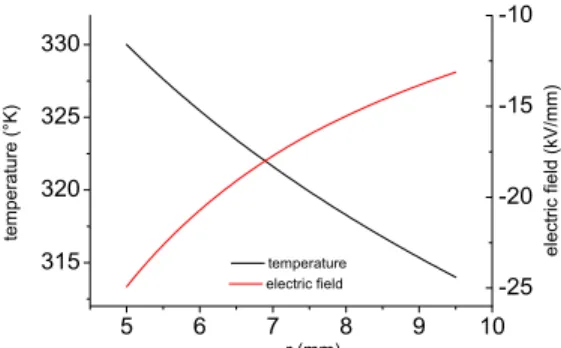
A MV cable, made from cross-linked polyethylene (XLPE) of thickness 4.5 mm is simulated using the different models. The inner insulation radius is 5 mm, the outer radius is 9.5mm. A temperature gradient can be applied on the cable. When the temperature gradient is dT=16°C, the inner electrode is at T=57°C and the outer at 41°C. The applied voltage at the inner electrode is -80 kV. The outer electrode is grounded. Fig. 1 represents the geometric electric field distribution and the temperature distribution inside the cable for the example of a cable polarized at -80 kV and a dT=16°C.
Fig. 1. Temperature distribution and electric field distribution in a MV cable of 4.5mm polarized at -80 kV, with a temperature gradient of ΔT=16°C.
III. MODELS DESCRIPTION
A. Charge transport models
The bipolar model has already been presented elsewhere [7] and features the bipolar injection of electronic carriers at the electrodes, conduction between shallow traps via a field and temperature dependent mobility (hopping), trapping into deep traps, detrapping and recombination, function of the carriers mobility (Langevin) (Fig. 2). For sake of simplification, internal generation (dissociation) is not taken into account in the simulations. The equations to solve are of the form, neglecting diffusion:
ja(r, t) = na,µ(r, t)µa(r, t)E(r, t) Transport (1)
where a refers to the type of charge, i.e. electron or hole and r is the cable radius. j is the conduction current density for each kind of carriers, naµ is the mobile density of charge. µ refers to the mobility, E is the electric field and t the time.
dE(r, t) dr = ρ(r, t) ε0εr Poisson equation (2) ∂na(r, t) ∂t + ∂ja(r, t) ∂r = sa(r, t) convection-diffusion (3)
ρ is the net charge density,
ε
0the vacuum permittivity, andr
ε
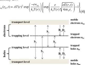
the dielectric permittivity. sa are the source terms, which encompass the changes in local density by processes other than transport (trapping, detrapping, etc). Charge generation is only by injection at each electrode, and follows the modified Schottky law: 2 0 0 ( , ) ( , ) ( ) exp exp 1 ( ) ( ) 4 inj inj i b b r ew e eE r t j r t AT r k T r k T r πε ε ⎧ ⎛ ⎞ ⎫ − ⎛ ⎞ ⎪ ⎪ = ⎜ ⎟⎨ ⎜⎜ ⎟⎟− ⎬ ⎝ ⎠ ⎪⎩ ⎝ ⎠ ⎪⎭(4)
where A is the Richardson constant, ri0 corresponds to the interface coordinate, and winj is the injection barrier height. kB is the Boltzmann constant, T the temperature, and E(r,t) the electric field at the electrode at position r. The extraction of charges is possible at each electrode, and follows an ohmic law.
The temperature distribution within the cable is calculated using the following equation:
T(r) = T(ri) − ln r ri " # $ % & ' T(r
(
i) − T(ro))
ln ro ri " # $ % & ' (5) where T(ri) and T(ro) are the temperature at the inner and theouter electrode, respectively.
For all the simulations, the parameters taken into account are the one of [7] for LDPE based materials. No attempt has been made to optimize the set of parameters to fit to XLPE results. The only requirement was to have a mean hopping mobility (electrons-holes) of the same order of magnitude as the one fitted by the macroscopic model, for a given electric field, which was the case with the parameters used.
1. FVM 'homemade' model
The description of the 'homemade' model has already been published in [7]. It is a Finite Volume explicit code, using a third order accuracy in space and fourth order in time. The grid to discretize the insulating material is divided into 301 elements, non-uniform, having a smaller size when approaching the electrodes. A flux limiter (ULTIMATE) is used to correct the charge flux within the dielectric. The time steps follow the CFL condition.
2. FEM 1D axisymmetric model
The model, developed with COMSOL Multiphysics® uses the Transport of Diluted Species (TDS) module to solve the convection-diffusion equation for each kind of carrier (4). The advantage of this module is that it already includes solutions to stabilize the solution and to prevent oscillations (i.e. negative densities). The mathematic module is used to couple these equations to the Poisson equation. Backward Difference F solver is used for the time integration (maximum order 2, and minimum order 1). The discretization grid is divided into 9000 elements of 0.5 µm each.
B. Macroscopic model
The input data used in the macroscopic approach are issued from conductivity measurements realized in a previous work [8]. For each of the materials, the conductivity was estimated after 1 h charging time as a function of temperature (20 to 90 °C) and field (from 2 up to 30 kV/mm), on 500 µm-thick samples metallized with gold electrodes. These experimental data were fitted with a conductivity law of the type:
transport level mobileelectrons neµ
trapped electrons net trapped holes nht mobile holes nhµ S3 S22 S1 S0 Bee Bhh Dee Dhh el ect ro n s trapping level ho le s trapping level transport level
Fig. 2. Schematic representation of the two-level transport model. Conduction is by free charges in the transport levels, associated with a hopping mobility between shallow traps. Deep trapping is taken into account through the existence of a single trapping level for each kind of carriers, electrons and holes. Si, Bi and Di are recombination (Langevin),
trapping and de-trapping coefficients respectively. ni is the carrier density
in transport and trapping levels. Indexes e and h refer to electrons and holes; µ ant t refer to mobile and trapped charges.
σ(T, E) = A exp − Ea kBT # $ % & ' (sinh B(T).E( )Eα (6)
where E is the field, T is the temperature, kB is the Boltzmann’s constant and the other symbols are coefficients with values taken from [8]. In this model, two different modules of COMSOL Multiphysics® (Heat transfer and electric currents) have been coupled. Heat transfer consists in the exchange of thermal energy between physical systems. The heat transfer rate is dependent on the systems temperatures and on the properties of the involved medium through which the heat is transferred. The electric currents module allows solving the current equation considering the electrical potential as a reference under DC or AC stress.
IV. RESULTS
A. Comparison between FVM and FEM results
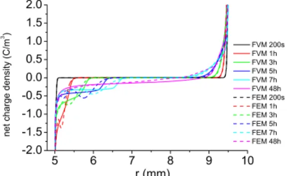
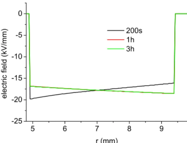
Simulations have been performed for a MV cable polarized at -80 kV and a dT=16°C, for 48h, using the FVM model and the FEM model, with the same parameters. Figure 3 presents the comparison of the simulated electric fields as a function of the radius of the cable at different times. At times below 5 hours, both models give globally the same electric field distributions. Some differences already appear, on the location of the maximum of the electric field, and the maximal value. This difference is less than 1% in position, and around 2% in value for 5hours. However, when increasing the simulation time, the difference between FEM and FVM becomes substantial, leading to a maximum of electric field located in the middle of the dielectric for the case of FEM, whereas it is next to the outer electrode for the FVM method. Net charge density as a function of radius is also presented (Figure 4) for the same times of simulation. It seems that the FVM model smoothes the net charge density compared to the FEM model, which is surprising, as the scheme used is not known for having a high numerical diffusion. On the contrary, the FEM results show oscillations, which are not due to physical processes (packets). Simulations have been performed for plane/parallel geometry for each model, leading to similar results for each model. This validates the FEM model development, the FVM model having already been validated in different publications. The specific case of cable geometry, with a non-uniform electric field and temperature, increases the differences, notably at the inner interface, where charge generation is enhanced by the high temperature and field. A small difference in this boundary condition has a huge impact on the simulated data. Other causes could be found (discretization errors, diffusion, meshing...), without knowing at the moment which one has the most significant impact on the simulation results.
B. Comparison between fluid and macroscopic models
Electric field distribution vs. radius has been simulated for a XLPE material using the macroscopic model (Figure 5) [8]. These results are to be compared to those of Figure 3, issued from fluid models. Different processes are at play in the bipolar fluid models, with variable characteristic times for each process. At short times, injection is the most important process, while trapping/detrapping becomes more important at
Fig. 3. Electric field distribution vs. radius for different times of simulation, for the FVM model (lines), and for the FEM model (dotted lines) for a MV cable of 4.5mm thick insulation polarized at -80 kV, and a temperature gradient of ΔT=16°C.
Fig. 4. Net charge density vs. radius for different times of simulation, for the FVM model (lines), and for the FEM model (dotted lines) for a MV cable of 4.5mm thick insulation polarized at -80 kV, and a temperature gradient of ΔT=16°C.
longer times. On the other side, only a mean conductivity drives the charge dynamics in the macroscopic model. We then choose to compare the electric field distributions at stationary states for each model, not regarding the transient results. Both models (macroscopic and fluid) are able to predict the change in the location of the maximal field that changes from the inner electrode (Laplacien Field) to the outer electrode with time. The maximal and minimal values are however overestimated in the fluid models compared to the macroscopic model, the maximal electric field reaching 22.5 kV/mm in the case of the fluid model (FVM), whereas the maximal value in the case of the macroscopic model is less than 20 kV/mm. Moreover, both fluid models (FVM and FEM) predict an electric field being almost 0 at the inner electrode, which is not the case in the macroscopic model, where the electric field minimum is of the order of 17 kV/mm. Fluid models, taking into account charge injection and accumulation (homocharges in this case) allow having such a variation of the electric field whereas the macroscopic model results will remain in the limits fixed by the conductivity variation linked to the thermal and/or electrical gradient. However, the parameterization for the fluid models, the physics behind, is not straightforward to implement. Besides, it requires a long computation time, compared to macroscopic models.
Fig. 5. Electric field distribution vs. radius for different times of simulation, for the macroscopic model and for a MV cable of 4.5mm thick polarized at -80 kV, and a temperature gradient of ΔT=16°C.
C. Comparison between experimental and simulated electric field distribution
Space charge measurements have also been performed for this specific protocol, on MV cables polarized at -80 kV for a temperature gradient of dT=16°C [9]. The Poisson equation (2) allows obtaining the measured field distribution as a function of cable radius for different times (Figure 6). The maximal value of the electric field, initially located at the inner electrode, is observed at the outer electrode after 2h of applied voltage. The maximal value is around 22 kV/mm after 3 hours, while another peak appears at the inner electrode, due to positive heterocharges accumulating there. When comparing the simulated results to the experimental ones, the location of the maximal electric field is predicted. The value of this electric field is however underestimated in the case of the macroscopic model, while the fluid models prediction is consistent. However, the charge dynamics is excessively low in the fluid models (due to a non optimization of the parameters for XLPE among other possible explanations). Macroscopic and fluid models fail to reproduce the increase in the electric field at the inner electrode with time. The macroscopic model will never be able to predict it, as only based on conductivity variation. The fluid models could predict this peak if either barrier to extraction or ionic species were considered in as physical processes.
V. CONCLUSION
Two fluid models, a Finite Volume code and a Finite Element code, have been developed and compared as regards a real situation, i.e. a MV cable geometry with a thermal gradient. Comparison between FEM and FVM model shows discrepancy in the electric field distribution that increases with the simulation time. Even for steady state, the simulation results are not totally consistent. This shows at first the need to take care of the numerical resolution of the model. On this area, more work needs to be done to improve the FEM model. Comparing fluid models to macroscopic ones by means of electric field distribution shows the strengths and drawbacks
of each approach, i.e. easy implementation of the conductivity and short time simulations in the case of macroscopic models, while limited when charge accumulation comes at play. On the other side, the complex physics/complex parameterization/long lasting simulation drawbacks are counterbalanced by an efficient description of the charge behaviour.
Fig. 6. Measured (PEA) electric field distribution vs. radius for different times, for a MV cable of 4.5mm polarized at -80 kV, and a temperature gradient of ΔT=16°C.
ACKNOWLEDGEMENTS
We would like to acknowledge the C.N.R.S. for financial support from the PICS project ModHVDC n° 07965
REFERENCES
[1] J.M. Alison and R.M. Hill J. Phys. D: Appl. Phys. 27 1291-9, 1994. [2] K Kaneko, Y. Suzuoki and T. Mizutani IEEE Trans. Diel. Elec. Insul. 6 152-8, 1999.
[3] M. Fukuma, M. Nagao and M. Kosaki Proc. 4th International Conference on Properties and Applications of Dielectric Materials (Brisbane) pp 24-7, 1994.
[4] J. Xia, Y. Zhang, F. Zheng, Z. An and Q. Lei, “Numerical analysis of packetlike charge behavior in low-density polyethylene by a Gunn Effectlike model”, J. Appl. Phys., vol 109, 034101 (9p), 2011.
[5] A.T. Hoang, Y.V. Serdyuk and S. Gubanski, “Charge transport in LDPE nanocomposites Part II - Computational approach”, Polymers, vol. 8, 103 (16p), 2016.
[6] D. Min, W. Wang and S. Li, “Numerical analysis of space charge accumulation and conduction properties in LDPE nanodielectrics”, IEEE Trans. Dielectr. Electr. Insul., vol. 22, 1483–1491, 2015.
[7] S. Le Roy, G. Teyssedre and C. Laurent, “Modelling space charge in a cable geometry”, IEEE Trans. Dielectr. Electr. Insul., vol. 23, pp. 2361−2367, 2016.
[8] T.T.N. Vu, G. Teyssedre, S. Le Roy and C. Laurent, “Maxwell-Wagner effect in multi-layered dielectrics: interfacial charge measurement and modelling”, Technologies, vol. 5, pp.1-14, 2017.
[9] T.T.N. Vu, G. Teyssedre, B. Vissouvanadin, S. Le Roy, C. Laurent, M. Mammeri, I. Denizet, "Field distribution under temperature gradient in polymeric MV-HVDC model cable: simulation and space charge measurements", Eur J. Electr. Engg. Vol. 17, 307-325, 2014.