For Peer Review Only
Dynamics of groundwater floodwaves and groundwater flood events in an alluvial aquifer.
Journal: Canadian Water Resources Journal Manuscript ID: TCWR-2014-0084.R2
Manuscript Type: Original Paper Date Submitted by the Author: n/a
Complete List of Authors: Buffin-Bélanger, Thomas; UQAR, Biologie, chimie et géographie Cloutier, Claude-André; UQAR, Biologie, chimie et géographie Tremblay, Catherine; UQAR, Biologie, chimie et géographie Chaillou, Gwenaëlle; UQAR, Biologie, chimie et géographie Larocque, Marie; UQAM, Sciences de la Terre et de l'atmosphère
Keywords: groundwater floodwave, groundwater flood event, floodplain, groundwater - surface interactions
For Peer Review Only
1
Dynamics of groundwater floodwaves and groundwater flood events in
2
an alluvial aquifer.
3 4 5 6 7Thomas Buffin-Bélanger1, Claude-André Cloutier1, Catherine Tremblay1, Gwénaëlle 8
Chaillou1 and Marie Larocque2 9
10
1
Département de biologie, chimie et géographie, Université du Québec à Rimouski, 11
Rimouski, Québec, Canada G5L 3A1 12
13
2
Centre de recherche GÉOTOP, Département des sciences de la Terre et de 14
l’atmosphère, Université du Québec à Montréal, Montréal, Québec, Canada H2C 3P8 15
16
Abstract
17
In gravelly floodplains, streamflood events induce groundwater floodwaves that 18
propagate through the alluvial aquifer. Understanding groundwater floodwave dynamics 19
can contribute to groundwater flood risk management. This study documents 20
groundwater floodwaves at a flood event basis to fully assess environmental factors that 21
control their propagation velocity, their amplitude, and their extension in the floodplain, 22
and examines the expression of groundwater flooding in the Matane River floodplain 23
(Québec, Canada). An array of 15 piezometers equipped with automated level sensors 24
and a river stage gauge monitoring at 15-minute intervals from September 2011 to 25
September 2014 were installed within a 0.04 km2 area of the floodplain. Cross-correlation 26
analyses were performed between piezometric and river level time series for 54 flood 27
events. The results revealed that groundwater floodwave propagation occurs at all flood 28
magnitudes. The smaller floods produced a clear groundwater floodwave through the 29
floodplain while the largest floods affected local groundwater flow orientation by 30
generating an inversion of the hydraulic gradient. Propagation velocities ranging from 8 31
to 13 m/h, which are two to three orders of magnitude higher than groundwater velocity, 32
were documented while the induced pulse propagated across the floodplain to more than 33
230 m from the channel. Propagation velocity and amplitude attenuation of the 34
For Peer Review Only
groundwater floodwaves depend both on flood event characteristics and the aquifer 35
characteristics. Groundwater flooding events are documented at discharge (< 0.5 Qbf). 36
This study highlights the role of flood event hydrographs and environmental variables on 37
groundwater floodwave properties and the complex relationship between flood event 38
discharge and groundwater flooding. The role that groundwater floodwaves play in flood 39
mapping and the ability of analytical solutions to reproduce them are also discussed. 40
Résumé:
41
Les crues provoquent la propagation d’ondes phréatiques dans les aquifères alluviaux. 42
Comprendre la dynamique des ondes phréatiques peut contribuer à la gestion des risques 43
d’inondation par rehaussement de la nappe. Cette étude documente des ondes phréatiques 44
à l’échelle événementielle pour évaluer les facteurs environnementaux contrôlant leur 45
vitesse de propagation, leur amplitude et leur extension dans la plaine alluviale, et 46
examine des inondations par rehaussement de la nappe dans la plaine alluviale de la 47
rivière Matane (Québec, Canada). Quinze piézomètres équipés de capteurs de pression 48
hydrostatique et une station de jaugeage ont été installés dans une portion de la plaine 49
alluviale et la rivière Matane. Les mesures ont été prises toutes les 15 minutes de 50
Septembre 2011 à Septembre 2014. Les corrélations-croisées entre les niveaux 51
piézométriques et de la rivière de 54 événements de crues révèlent la propagation d’une 52
onde phréatique à toutes les crues. L’étude du gradient hydraulique révèle que les plus 53
grandes crues engendrent également une inversion de l’écoulement souterrain dans la 54
plaine. Des vitesses de propagation de 8 à 13 m / h, soit de deux à trois ordres de 55
grandeur plus élevés que l’écoulement de l’eau souterraine, sont observées et se 56
propagent à travers la plaine à plus de 230 m de la rivière. Des événements d’inondation 57
par rehaussement de la nappe sont documentés à des événements de crues bien en 58
dessous du niveau plein bord. Cette étude met en évidence le rôle de la forme des 59
hydrogrammes et des variables environnementales sur les ondes phréatiques et révèle la 60
relation complexe entre l’amplitude des crues et les inondations par rehaussement de la 61
nappe phréatique. Le rôle des ondes phréatiques pour la cartographie des inondations par 62
rehaussement de la nappe et la capacité des solutions analytiques pour les reproduire sont 63
également discutés. 64
For Peer Review Only
65
INTRODUCTION
66
Hydrostatic and hydrodynamic processes govern a wide range of interactions between 67
surface water and groundwater in gravelly floodplains. Among the interactions that occur 68
between the groundwater and surface water is the groundwater floodwave that propagates 69
through floodplains following rapid changes in river stage. The mechanisms of hydraulic 70
pressure head propagations through floodplain environments have been discussed by 71
previous studies (Sophocleous 1991; Vekerdy and Meijerink 1998; Jung et al. 2004; 72
Lewandowski et al. 2009; Vidon 2012; Cloutier et al. 2014). The pressure wave effect 73
was revealed by observations of rapid changes in groundwater levels due to flood event at 74
distances from the river that cannot be explained by Darcian velocities. Several authors 75
have observed propagation velocities that are two to three orders or magnitude higher 76
than groundwater velocities (Jung et al. 2004; Lewandowski et al. 2009; Vidon, 2012; 77
Cloutier et al. 2014). Groundwater floodwaves can be interpreted either as kinematic 78
waves (i.e. Jung et al. 2004) or dynamic waves (Vekerdy and Meijerink 1998; Cloutier et 79
al. 2014), depending on the dispersive and diffusive behaviour of the floodwave 80
propagation. 81
Groundwater floodwaves are part of the hydrological response of a river corridor. They 82
can indicate the degree of wetland-to-river connectivity where the floodplain material is 83
highly permeable (Larocque et al. submitted), they are critical in revealing the occurrence 84
and duration of intense biogeochemical transformations (Vidon 2012), and they are a key 85
element in the delineation of groundwater flooding (Cloutier et al. 2014). Groundwater 86
flooding has no substantial effect on river or floodplain morphology, but it is typically of 87
a longer duration than overbank flooding and can find its way into basements as well as 88
block roads and railways. Groundwater flooding is largely recognized as a flooding 89
process that can cause severe consequences to man-made infrastructures in chalk systems 90
(e.g., Finch et al. 2004; Cobby et al. 2009), and groundwater hazard and risk maps are 91
available for such consolidated aquifers (Hughes et al. 2011). However, groundwater 92
flooding from an alluvial aquifer connected to high river levels is still a poorly 93
For Peer Review Only
understood flooding process (Macdonald et al. 2012) when compared to processes such 94
as overbank flooding and ice- or log-jam flooding which perform geomorphic work on 95
floodplains that provide evidence for assessing the extent of flooded areas (Demers et al. 96
2014). Furthermore, groundwater flooding may occur far beyond the hyporheic zone, 97
where there is no direct groundwater – surface water connection (Mertes 1997). 98
Groundwater flooding can be due to the propagation of groundwater floodwave when the 99
water table rise is greater than the thickness of the unsaturated zone. Groundwater 100
flooding is controlled by factors that include floodplain morphology, the initial 101
thickness of the unsaturated zone, hydraulic properties of the floodplain geology, and 102
groundwater inflow from a regional aquifer (Macdonald et al. 2012). Morphological units 103
such as abandoned channels, overflow channels, or swales represent floodplain features 104
susceptible to groundwater flooding. These units are generally below bankfull levels and 105
can be considered as negative reliefs (Lewin and Ashworth 2014); they may be saturated 106
prior to the streamflood crest. A better understanding of groundwater floodwave 107
propagation is needed to determine the extent and frequency of groundwater flooding in 108
alluvial aquifers. 109
Groundwater floodwaves have been documented using both field studies (Lewandowski 110
et al. 2009; Vidon 2012; Cloutier et al. 2014) and analytical solutions (Ha et al. 2008; 111
Dong et al. 2013). Using arrays of piezometers, Vidon (2012) and Cloutier et al. (2014) 112
studied the groundwater level fluctuations in response to a series of flood events in the 113
sandy floodplain of Fishback Creek (Indiana, USA) and in the gravelly floodplain of the 114
Matane River (Québec, Canada), respectively. In these unconfined aquifers, they showed 115
that groundwater level rises occurred at a time lag that was proportional to the distance 116
between a piezometer and the river. This finding was explained by the presence of a 117
groundwater floodwave controlled by river stage rather than by precipitation. Cross-118
correlation analysis between precipitation and groundwater levels showed significantly 119
lower correlation values (r= 0.2–0.3) than those from cross-correlation analysis between 120
river stage and groundwater levels (r>0.9) (Cloutier et al. 2014). Both studies also 121
revealed that groundwater floodwave amplitudes decrease with distance from the river 122
bank, but that the ratio of river stage amplitude to groundwater amplitude was 123
independent of the flood event magnitude and that a hydraulic gradient inversion occurs 124
For Peer Review Only
at the highest flood events. In confined aquifers, pressure transfer is almost instantaneous 125
compared to unconfined aquifers where lags can be much higher (Lewandowski et al. 126
2009) and propagation slower (Vekerdy and Mejerink 1998). In the unconfined Matane 127
River aquifer, the propagation velocity remains relatively constant but is affected by 128
conditions of the unsaturated zone before a flood event (Cloutier et al. 2014). 129
Using analytical solutions, Ha et al. (2008) showed that the shape of flood hydrographs 130
plays an important role in bank storage and discharge. The shape of flood hydrographs is 131
strongly related to environmental factors, ranging from drainage basin areas to rainfall 132
structures. They suggest that river water infiltration into the aquifer and bank storage 133
increase with river stage and flood duration. Similarly, Dong et al. (2013) suggested that 134
the difference in response time might result from different hydrographic geometries such 135
that rapid river stage variations will promote quicker groundwater responses. The shape 136
of hydrographs generated by analytical solutions are generally asymmetrical but they 137
rarely consider the full complexity of natural and successive flood events. However, 138
propagation velocity is not only related to the geometry of the flood hydrograph. Using 139
analytical solutions, Dong et al. (2013) showed that the propagation velocity of 140
groundwater floodwave is proportional to the aquifer diffusivity as well as the distance at 141
which the wave propagates in the floodplain. They calculated propagation velocities from 142
0.5 to 8 m/h for aquifer diffusivities from 0.4 to 50 m2/h, respectively. 143
Field studies and analytical solutions highlight the need to fully assess the role of 144
environmental factors through the use of field data on propagation velocity, amplitude, 145
and the lateral extent of the groundwater floodwave (Ghasemizade and Shirmer, 2013). 146
The aim of this study is to document the key properties of groundwater floodwaves in a 147
gravelly alluvial aquifer. While Vidon (2012) and Cloutier et al. (2014) focused on seven 148
flood events, this study analyses a three-year dataset that includes 54 flood events. The 149
study relies on time series analysis of hydraulic heads measured at fifteen locations in the 150
floodplain. The large number of flood events provides a wide array of conditions from 151
which to identify the key factors influencing groundwater floodwaves. The role that 152
groundwater floodwaves play in flood mapping and the ability of analytical solutions to 153
reproduce them are discussed. 154
For Peer Review Only
MATERIALS AND METHODS155
Study site
156
The Matane River valley is located on the northwest portion of the Gaspé Peninsula, in 157
eastern Québec, Canada (Figure 1a). The Matane River system is a 1678 km2 basin 158
flowing from the Notre-Dame mountain range to the south shore of the St. Lawrence 159
Estuary. The flow regime of the Matane River is nivo-pluvial, with two periods of high 160
discharges; the first occurring at snowmelt in May and the second occurring in the fall 161
when rain events are more frequent and vegetation less active. Bankfull discharge (Qbf) is
162
estimated at 350 m3/s, the mean annual river discharge is 39 m3/s (1929–2009), and the 163
minimum discharge (considered as baseflow) is on the order of 5 m3/s. Discharge values 164
are available from the Matane gauging station operated by the Centre d’expertise 165
hydrique du Québec (CEHQ 2014; station 021601). The climate normal for the 1981– 166
2010 period indicate an average daily temperature of 2°C and total annual precipitation of 167
1032 mm (Environment Canada 2014; Amqui station). For the three-year study period 168
(2011-2014), average daily temperature was 3°C while average annual total precipitation 169
was 1052 mm (Ministère du Développement durable, de l’Environnement et de la lutte 170
contre les changements climatiques, 2014; Station 7057692). 171
The lithology of the Matane valley is deformed sedimentary rock associated with the 172
Appalachian orogenesis from the Cambro-Ordovician period. The irregular meandering 173
planform flows into a wide semi-alluvial valley cut into recent fluvial deposits (Lebuis 174
1973; Marchand et al. 2014; Fig. 1b). The entire floodplain of the Matane River consist 175
of gravel deposits from lateral migration of the meandering river on top of which thin 176
layers of overbank deposits are found. The mean channel and valley width are 55 m and 177
475 m, respectively, and the average river gradient is 0.2 (m/100m). According to 178
borehole data from the valley floor, the average unconsolidated sediment thickness is 49 179
m. The entire alluvial aquifer of the Matane valley is an unconfined coarse sand/gravel 180
and pebble aquifer with a mean saturated thickness of 46 m, except near the city of 181
Matane, where the alluvial aquifer is overlaid by a 30 m thick silty/clay marine deposit. 182
For Peer Review Only
The study site, located 28 km upstream from the estuary (48° 40' 5.678" N, 67° 21' 183
12.34" W), is characterized by an elongated depression that corresponds to the abandoned 184
channel and a few overflow channels (Figure 1c). These morphologic features are part of 185
the wetland, and its characteristics are fully described in Larocque et al. (submitted). The 186
floodplain is very low, with the deepest parts of the depression being lower than the river 187
water level at discharges well below bankfull. The mean groundwater level at the study 188
site is 58.8 m above mean sea level, whereas the average surface elevation of the 189
floodplain is 60.4 m above sea level, i.e., the average unsaturated zone is 1.6 m. A 190
borehole next to the study site revealed that the unconfined alluvial aquifer thickness is 191
47.4 m overlying a 7 m till deposit over the bedrock. The aquifer consists of coarse sands 192
and gravels covered by overbank sand deposit layers of variable thickness, from 0.30 m 193
at the top of high ground to 0.75 m within abandoned channels. At the regional scale, 194
equipotential lines follow those of the topography, thus the Matane River is draining the 195
regional aquifer. At the study site, the Matane River is a gaining stream, i.e., the 196
groundwater flow gradient is towards the river. However, hydraulic gradients can change 197
drastically, whilst the gradient can temporarily be from the river towards the valley wall 198
at high flows (Cloutier et al. 2014). 199
Data collection
200
An array of 15 piezometers equipped with pressure sensors were installed in a 0.04 km2 201
area on the study site (Figure 1c). The piezometers were made from 38 mm ID PVC 202
pipes sealed at the base and equipped with a 0.3 m screen at the bottom end. At every 203
location, piezometers reached 3 m below the surface but because of the surface 204
microtopography, the piezometer bottoms reached various depths within the alluvial 205
aquifer (Table 1). However, the bottom end would always be at or below the altitude of 206
the river bed (58.4 m). Piezometer locations and altitudes were determined using a 207
Magellan ProMark III differential GPS. At each location, hydraulic conductivities (K) 208
were derived from slug tests using the Hvorslev (1951) method. Hydraulic diffusivity (D) 209
was estimated from the ratio of transitivity (T=Kb where b=saturated thickness) to the 210
storage coefficient (S). Automated level loggers (Hobo U20-001) recorded groundwater 211
levels every 15 minutes from 1st September 2011 to 10th September 2014 (3 hydrological 212
For Peer Review Only
years) and from 6th July 2012 to 10th September 2014 (2 hydrological years) for 10 and 5 213
piezometers, respectively. Table 1 shows the period of operation of each pressure sensor 214
and the proportion of valid data. A river stage gauge was installed in the upstream section 215
of the study site where river banks and bed are stable (Figure 1c) and recorded water 216
levels every 15 min from September 2011 to September 2014. The upstream location of 217
the river gauge implies that the water level in the river will always be at a higher 218
elevation than the water table elevation that is measured within the study site. Time series 219
were corrected for barometric pressure from a barologger located at the study site (Figure 220
1c). Finally, an automatic camera (Reconix Hyperfire PC800) was installed in January 221
2013 to monitor the presence of water on the floodplain surface (Bertoldi et al., 2012). 222
The camera was installed to focus on the depression in the eastern section of the study 223
site (Figure 1c). Pictures were taken every hour during the sampling period. 224
Data analysis
225
Figure 2a shows the river stage time series and selected groundwater level time series 226
from three piezometers located at various distances from the river for the 3 years 227
sampling period. River stages values are higher than the water table values because of the 228
upstream location of the river gauge. Strong correlation can be observed between 229
groundwater levels and river stage at a wide range of flood magnitudes. Figure 2b shows 230
for a shorter time period that there is an increasing time lag with distance from the river 231
between the maximum groundwater level and the maximum river stage. Surface water – 232
groundwater interactions and floodwave propagation in floodplain environments have 233
been studied using analytical solutions (Cooper and Rorabaugh, 1963; Vekerdy and 234
Meijerink, 1998; Ha et al. 2008; Dong et al. 2013), principal component analysis 235
(Lewandowski et al. 2009), cross-correlation analysis (Cloutier et al. 2014; Larocque et 236
al. submitted), and numerical modelling (Sophocleous 1991; Bates et al. 2000). Cross-237
correlations are widely used to quantify (1) the intensity of the relationship between river 238
stage and groundwater levels and (2) the time lag between the maximum groundwater 239
levels and the maximum river stage (Larocque et al. 1998; Vidon 2012; Cloutier et al. 240
2014). A cross-correlation can be computed for the entire time series (Larocque et al. 241
For Peer Review Only
submitted) or for an individual flood event (Cloutier et al. 2014), thus providing 242
information on different scales of interactions between groundwater and surface water. 243
Here, cross-correlation analyses between the river stage and groundwater levels at every 244
location were undertaken for individual flood events. Flood events were selected based 245
on a significant change of river stage (> 4 cm), a minimum duration (> 60 hours), and 246
minimum rising limb duration (> 10 hours). The end point of a flood event was 247
determined from either the beginning of a new event or the return of the flow stage to 248
pre-event values. Care was also taken to avoid complex responses due to multiple rain 249
events occurring over short time intervals. As an example, Figure 2b illustrates three 250
flood events selected and the other three flood events rejected between 20 September and 251
15 November 2013. In this example, flood events before and after 15 October were not 252
selected because of small changes in river stage or because of a complex river stage 253
response. Using these criteria, 54 flood events were selected for the cross-correlation 254
analysis (Figure 2a). Median flood event duration, median rising limb duration, and 255
median river stage amplitude for the 54 flood events were 200 h, 27 h, and 0.34 m, 256
respectively. 257
For each selected flood event, the time lag at which the maximum correlation (rxy_max)
258
occurred between groundwater level and river stage was extracted for each piezometer. 259
The relationship between the time lag at rxy_max and the perpendicular distance from the
260
piezometer to the river allows computation of the velocity at which the crest of the 261
floodwave propagates through the aquifer (Cloutier et al. 2014). Because of the large 262
number of flood events considered in this study, velocity propagation was examined in 263
relation to characteristics of the flood events, including initial river and groundwater 264
levels, length of the rising limb, maximum river stage reached during the flood, flood 265
duration, time since the previous flood event, and amplitude, i.e., the maximum river 266
stage minus the initial river stage. 267
Hydraulic heads were used to compute hydraulic gradients in the floodplain. Vidon 268
(2012) and Cloutier et al. (2014) illustrated the inversions of hydraulic gradient in the 269
floodplain at high river stages using piezometric maps at specific time steps during a 270
For Peer Review Only
flood event. Here, linear regressions between groundwater levels recorded at all 271
piezometers and the perpendicular distance to the river were calculated at every time step 272
to produce continuous time series of hydraulic gradients. Positive gradients indicate that 273
groundwater levels increase towards the valley side and thus that the floodplain is 274
discharging in the river (gaining stream); negative gradients indicate that bank storage is 275
in process (losing stream). The use of all groundwater levels represents a way to integrate 276
the water level fluctuations within the entire floodplain. 277
The occurrence of groundwater flooding was evaluated using difference between the 278
water level recorded by the automated level loggers in the piezometers and the 279
topography at the each piezometer location. A positive value suggests that there is water 280
above the ground. When this occurs, it is assumed that the water on the surface is the 281
expression of high water table since the floodplain is fully saturated at the piezometer 282
location. The automatic camera was used to confirm the presence of water at one location 283
on the study site. Groundwater levels are mapped for the flood event allowing 284
visualization of the spatial extent and depth of groundwater flooding. Similar methods 285
using topographic depression and water levels were used by Macdonald et al. (2012) to 286
map the extent and location of groundwater flooding. 287
RESULTS
288
Propagation velocities from cross-correlation analysis
289
Propagation velocity was computed for all 54 flood events. Figure 3a shows a typical 290
relationship between the time lag of rxy_max and the perpendicular distance to the river for
291
a flood event. The linear relationship is highly significant (R2 = 0.91, p < 0.01) and has a 292
slope of 0.13 h/m. The propagation velocity is given by the inverse of the slope, which 293
for this event becomes 7.7 m/h. Seventy-five percent of all flood events have a R2 higher 294
than 0.80 while the median value for all flood events is 0.88 (Figure 3b). The strong 295
linear relationship between time lag and distance supports the use of the slope as an 296
estimation of propagation velocity for most flood events. The median propagation 297
velocity is 10.4 m/h while 50% of the propagation velocities lie between 8.2 and 13.5 m/h 298
(Figure 3c). 299
For Peer Review Only
Propagation velocity can also be computed by averaging the time lags for all flood events 300
at each piezometer (Figure 4a). There is a strong linear relationship between the averaged 301
time lags and distance from the river (R2 = 0.93, p-value < 0.01). The propagation 302
velocity computed from the slope of the relationship is 9.7 m/h and the strong linear 303
relationship suggests that the propagation velocity is relatively constant throughout the 304
floodplain. 305
The meander configuration at the study site (Figure 1c) suggests that the floodwave could 306
also be travelling from upstream to downstream within the floodplain. To investigate this 307
displacement, Figure 4b presents the distribution of averaged time lags when plotted 308
against the downstream distance between the river bank and the piezometers on the 309
floodplain. No pattern emerges from the scatter of points, and it seems clear that the main 310
advecting pattern during flood events is perpendicular to the river towards the valley side. 311
Groundwater floodwave amplitude attenuation
312
Figure 5 illustrates ways to look at amplitude attenuation as the floodwave propagates 313
thorough the floodplain. A strong relationship exists between the groundwater amplitude 314
and the flood event amplitude for all flood events and all piezometers (R2 = 0.65, p < 315
0.01; Figure 5a). There is significant attenuation of the groundwater amplitude recorded 316
within the floodplain with distance from the river bank (R2 = 0.60, p < 0.01; Figure 5b). 317
The groundwater amplitude decreases logarithmically from 0.30 m at 25 m to 0.20 m at 318
nearly 200 m from the bank. To examine the river stage amplitude for each flood event, 319
Figure 5c plots the ratio of groundwater to river stage amplitude in relation to the 320
piezometer’s distance from the bank. The logarithmic relationship is significant 321
(R2 = 0.85, p-value < 0.01), and suggests that the groundwater amplitude tends towards 322
50% of the flood event amplitude at the outer piezometers of the study site. 323
Flood event characteristics and floodwave propagation velocities
324
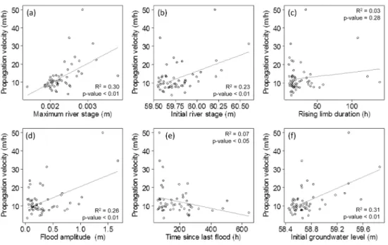
Figure 6 shows the groundwater floodwave propagation velocities in relation to flood 325
event characteristics. For illustration purposes, linear models are drawn on the scatter 326
plots. Propagation velocity appears to be positively related to maximum (R2 = 0.30, p-327
For Peer Review Only
value < 0.01) and initial (R2 = 0.23, p-value < 0.01) river stage, with flood amplitude 328
(R2 = 0.26, p-value < 0.01), and with initial groundwater level (R2 = 0.31, p < 0.01). 329
However, propagation velocity is inversely related to the time since last flood (R2 = 0.07, 330
p < 0.05) and has no significant relationship with the rising limb. 331
Relationships between propagation velocity and flood event characteristics are relatively 332
weak and are mainly influenced by the extreme values of the scatter plot. Furthermore, 333
flood event characteristics are strongly related to each other (for example, flood 334
amplitude is strongly linked to maximum river stage). It is thus difficult to consider them 335
separately. To consider the role of a combination of flood event characteristics, flood 336
events for the entire study period were classified by season of occurrence. Classifying the 337
flood event by season represents the integration into one variable of several factors 338
affecting the groundwater floodwave propagation. 339
When considering the distribution of propagation velocities according to the seasons for 340
all flood events (Figure 7a), winter must be interpreted carefully because only three 341
selected flood events occurred during that season (because of the presence of an ice cover 342
and accumulated snow generally between December and March/April) while 16, 21, and 343
14 selected flood events occurred during spring, summer, and fall, respectively. The 344
median propagation velocities and their seasonal variability (interquartile range) decrease 345
from spring to fall by 37 and 80%, respectively. The groundwater floodwave velocities 346
are larger (median = 13.4 m/h) and highly variable (interquartile range = 11.5 m/h) 347
during spring while being smaller (median = 8.4 m/h) and less variable (interquartile 348
range= 2.33 m/h) during fall. Linear relationships between the time lag and the distance 349
from the river for each piezometer and for the four seasons are shown on Figure 7b. For 350
all seasons except winter, linear relationships are relatively strong and significant. 351
Propagation velocities derived from the slopes are 11.1, 10.0, and 8.3 m/h for spring, 352
summer, and fall, respectively. These values are similar to those that would result from 353
averaging the slopes from all events (Figure 7a). The decreasing trend in propagation 354
velocity from spring to fall is particularly intriguing in light of the variability of flood 355
event characteristics. The propagation velocities are smaller for the fall period even 356
For Peer Review Only
though maximum and initial river stages, flood amplitude, and initial groundwater level 357
are not minimal during that season. 358
Hydraulic gradients
359
Hydraulic gradients were computed from the linear relationship between groundwater 360
levels and distances from the river to produce a continuous time series (Figure 8). Flood 361
event are indicated by the black triangle while the region where the hydraulic gradient is 362
not significantly different than 0 (1-α = 0.95) is located between the dashed lines. Figure 363
8a illustrates the hydraulic gradient time series for a two-month period (same period as 364
shown in Figure 2b). For that period, the hydraulic gradient was mainly from the river 365
towards the floodplain suggesting that bank storage was occurring. The higher negative 366
gradient during the flood event reveals the strong hydraulic gradient from the river 367
towards the aquifer. Figure 8b shows the changing nature of exchanges between the river 368
and the groundwater throughout the year. Considering only the hydraulic gradients that 369
are significant (60% of the sampling period), the floodplain discharges to the river more 370
than 69% of time while bank storage occurs 31% of the time. Bank storage, or negative 371
gradient, occurs for short period of time and is highly related to flood event as 41 of the 372
54 flood events are linked to bank storage processes. Season wise, the floodplain is 373
discharging to the river from December to July while bank storage is most important for 374
flood events occurring between July and November. 375
Groundwater flooding
376
Groundwater flooding was determined to occur when the piezometers measured 377
hydraulic head above the floodplain surface. This suggests that the unsaturated zone is 378
reduced to zero and that water can accumulate on the top of the saturated zone, above the 379
floodplain surface. Although the measured water levels in the piezometers represent 380
groundwater pressure, they are assumed to also reflect groundwater flooding because of 381
the high hydraulic conductivity of the floodplain deposits. To support this assumption, 382
the automatic camera confirmed the presence of water above the floodplain surface for 383
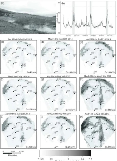
events where hydraulic head is measured as being above the floodplain surface. Figure 9a 384
shows a picture of groundwater flooding taken during the 254 m3/s flood event that 385
For Peer Review Only
occurred from April 22nd to May 8th 2014. As Matane river bankfull discharge is 386
estimated as 350 m3/s, no overflow occurred at the study site. Water can accumulate from 387
overland flow and precipitation, but the strong coherent patterns revealed by the 388
floodwave propagation analysis suggest that the surface ponding are linked to the water 389
table rising above ground level. Figure 10b illustrate the river stages at which 390
groundwater flooding occurred on the floodplain during the study period. Eight flood 391
events produced groundwater depth above the floodplain surface at various locations at 392
discharges well below bankfull, (Figure 9c to j), and only one flood event larger than 393
bankfull occurred at the study site (Figure 9k). Groundwater flooding always occurred in 394
the lowest parts of the floodplain, which includes the abandoned meander loop and the 395
overflow channel features. The elevations of these features (Figure 1c) are below the 396
bankfull level elevation of 60.6 m. The largest flood event (374 m3/s; Figure 9k) 397
produced the highest expression of the water table, but no clear relationship exists 398
between peak discharges and groundwater flow in the floodplain, likely due to the initial 399
condition of hydraulic heads within the floodplain. For example, the 146 m3/s flood event 400
(Figure 9e) produced groundwater flooding of a larger magnitude than that of the 182 401
m3/s flood event (Figure 9g). 402
DISCUSSION
403
At the flood event scale, the cross-correlation analysis between the piezometric and river 404
level time series revealed the strong interaction between groundwater and surface water 405
in the gravelly floodplain study site of the Matane River. The analysis shows both the 406
increasing time lag at which maximum correlation occurs and the amplitude attenuation 407
with increasing distance from the river bank. These results indicate that the groundwater 408
floodwave is a dynamic wave that occurs over a wide range of flood event magnitudes. 409
From the relationship between the time lag and the location of the piezometer in the 410
floodplain, propagation velocities ranging between 8 and 13 m/h were documented, and 411
the induced pulse could propagate to more than 230 m from the channel across the 412
floodplain (four times the mean channel width). Similar velocities were observed by 413
Vekerdy and Meijerink (1998) over a floodplain of more than 8 km in width. In the 414
phreatic aquifer of the Danube, Vekerdy and Meijerink (1998) documented propagation 415
For Peer Review Only
velocities ranging from 6 to 9 m/h, with the larger velocities being closer to the river 416
banks. In the Matane River floodplain, the floodwave propagation velocity appears 417
constant throughout the floodplain, but this could be due to the smaller width of the 418
floodplain (300 m). For a smaller number of flood events (N=7), Cloutier et al. (2014) 419
reported propagation velocities between 7 and 12 m/h for flood events occurring in 420
summer and fall in the Matane River floodplain. The slightly larger propagation 421
velocities reported here could be due to the presence of several flood events occurring in 422
spring, when the largest values are observed. 423
By documenting a large number of flood events, this study sheds light on two dynamics 424
of groundwater floodwaves that are relevant for watershed management. The first 425
dynamic is how the flood event hydrographs affects groundwater wave properties. Flood 426
event characteristics impact the propagation velocity of groundwater floodwaves. When 427
considered individually, maximum river level and initial groundwater level are positively 428
related to propagation velocity. This suggests that a larger flood event will produce faster 429
floodwave propagation and that the higher the groundwater level in the floodplain, the 430
faster the floodwave will propagate. It is worth noting that the rising limb does not seem 431
to determine a significant impact on floodwave propagation velocity. Chen and Chen 432
(2003) ran simulations of the effect of hydrograph shapes on infiltration rates and bank 433
storage. They suggested that hydrographs with a sharp rise, a high stage and a long 434
duration led to larger infiltration rates and larger bank storage. Thus, hydrograph 435
properties can play an important role in the rate and volume of stream infiltration and 436
return flow. The present study supports these simulations by highlighting the effect of 437
flood event stages on floodwave velocity propagation. Higher velocities are likely to 438
produce a floodwave that propagates through the entire floodplain and thus increases the 439
bank storage zone. 440
Although significant variability was observed for groundwater floodwaves properties 441
(e.g. propagation velocities, groundwater amplitude), this study also revealed seasonal 442
patterns. It was found that much of the variability in groundwater floodwave propagation 443
velocity can be explained by a seasonal component. Grouping the events by season 444
allows the integration of both flood hydrograph geometries and environmental 445
For Peer Review Only
characteristics. Propagation velocities were then explained by a seasonal component. 446
Also, bank storage processes that were quantified by changes in hydraulic gradient within 447
the floodplain appear to be of larger amplitude for flood events occurring between July 448
and November. The results also showed that amplitude attenuation followed a similar 449
logarithmic decrease at all flood event amplitudes. This supports Vidon’s observation that 450
groundwater levels with amplitudes high enough to affect soil biogeochemistry occurred 451
at all flood event magnitudes (Vidon 2012). 452
The second dynamic relates to the complex relationship between flood event discharge 453
and groundwater flooding in a floodplain. In the current study, groundwater flooding 454
occurred to various extents for a total of 9 flood events. This study attempted to link 455
flood event discharges to groundwater flooding properties such as spatial distribution and 456
depth. However, the relationship between flood discharge and groundwater flooding is 457
complex, since groundwater flooding occurs at a variety of discharge rates below and 458
above bankfull. Most discharge producing groundwater flooding are below those 459
proposed by Cloutier et al. (2014) from linear relationships between groundwater levels 460
and flood event discharges for the 2011 summer and fall period. The combination of 461
initial groundwater levels and flood event amplitudes may provide an explanation of this 462
complex relationship. Most flood event amplitudes were below 0.5 m, but many ranged 463
between 0.5 and 1.5 m (Figure 6d) while the initial groundwater levels showed that the 464
average unsaturated zone was 1.6 m. Since groundwater flooding occurs when the water 465
table rise is greater than the thickness of the unsaturated zone, it is important to 466
characterise the pre-flood unsaturated zone thickness. For instance, this emphasizes the 467
fact that even the smallest flood event (40 m3/s [0.1 Qbf]) produced water table to rise
468
above the floodplain at piezometer D176 (Figure 9). The occurrence of groundwater 469
flooding and discharge below or above bankfull highlights the degree of connectivity 470
between the stream and its alluvial aquifer. Most importantly, these results provide 471
insight on the dominant factors for groundwater flooding processes in the Matane River 472
floodplain: 1) the topography, i.e., floodplain morphological features such as abandoned 473
meander loops or overflow channels below bankfull levels, and 2) the initial thickness of 474
the unsaturated zone before a flood event. 475
For Peer Review Only
Analytical solutions represent an avenue to examine the dynamics and extent of 476
groundwater floodwave and to propose adequate strategies for groundwater flooding 477
attenuation. As an illustration, the analytical solution proposed by Dong et al. (2013) was 478
implemented and used with one of the flood events documented in this study. Hydraulic 479
diffusivity (D) needs to be determined before applying the analytical solution. The 480
median hydraulic diffusivity at the study site is 527 m2/h while 50% of the values range 481
between 177 and 738 m2/h (Table 1). The median hydraulic diffusivity was used in the 482
analytical solution. 483
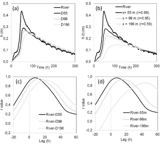
Figure 10a and b show the selected flood event with the measured and simulated 484
responses of the water table at 55, 98 and 196 m from the river bank (i.e. at specific 485
piezometer location). The simulated responses of the water table reflect the expected 486
decreasing amplitude of the water table fluctuation and the increasing time lag with 487
increasing distances from the river. However, it seems clear that the correspondence 488
between the simulated and the measured water table changes decreases with distance 489
from the river. Correlation coefficients calculated between the measured and the 490
simulated water levels are 0.99, 0.98 and 0.86 at distances of 55, 98 and 196 m, 491
respectively. The decreasing correspondence with distance is also revealed by the 492
comparison of measured and simulated cross-correlation functions between river levels 493
and piezometer levels (Figures 10c and 10d). Similar responses are observed at x=55 m 494
(max rxy(k) of 0.978 and 0.972 for observed and simulated time series respectively, and
495
similar delays of 7 hours for both time series) but adequacy decreases with distance from 496
the river. Adequacy is still good at x=96 m, although the max rxy(k) is slightly lower and
497
the delay is longer. At x=196 m, the adequacy between the measured and simulated 498
cross-correlations is significantly worst with slightly more attenuation and a delay that is 499
twice too long with the simulated data. As a result, the propagation velocity for the 500
measured floodwave (10.4 m/s) is twice the one for the simulated floodwave (4.1 m/s). 501
This discrepancy suggests that the use of D = 500 m2/h is adequate for distance of up to 502
100 m but that D changes beyond this distance. To obtain adequacy at the level of the 503
55m using Dong et al. (2013) analytical solution, the diffusivity has to be adjusted to 504
1100 m2/h and 2800 m2/h for the 98 m and 196 m distance, respectively. Several factors 505
could explain the need to adjust the diffusivity with distance from the river bank. The 506
For Peer Review Only
heterogeneity of hydraulic conductivity and diffusivity at the site (Table 1) and the 507
orientation of the floodwave within the floodplain are two of them (Ha et al. 2007). 508
Overall, however, the analytical solution with proper characteristics appears to be an 509
efficient tool to document how the floodwave propagates through the floodplain, if 510
sufficient data on the floodplain hydraulic properties are available. This suggests that the 511
propagation and the attenuation of a groundwater floodwave, and eventually the 512
groundwater flooding extension, could be calculated from anticipated events and hence 513
produce groundwater flooding maps. Only one event was used here for the discussion, 514
but the available dataset would allow to fully test analytical solutions such as the one 515
proposed by Dong et al. (2013). 516
Groundwater flood risk assessment in fluvial environments remains a challenge. More 517
data and a larger array of flood events are required to fully assess the mechanisms and 518
drivers involved in groundwater flooding as well as to develop adequate analytical 519
solutions. The assessment of groundwater flooding in an alluvial aquifer connected to 520
high river levels also remains an important challenge because this flooding process can 521
cause damage to man-made infrastructures. The high hydraulic connection between the 522
alluvial aquifer and the river suggests dynamics from both ways, i.e., streamfloods can 523
induce groundwater flooding, but the aquifer can drain easily at streamflood recession. A 524
better understanding of groundwater – surface water interactions may promote the 525
development of new management practices. For example, lateral connectivity between 526
groundwater and surface water tends to be recognized as a groundwater – river 527
continuum in the freedom space river management approach (Biron et al. 2014; Larocque 528
et al. submitted). This approach applies hydrogeomorphic principles to delineate zones 529
that are either frequently flooded or actively eroding, or that include riparian wetlands 530
and within which rivers are left free to evolve rather than being forced to flow in a 531
corridor shaped by human interventions. 532
CONCLUSION
533
The objective of this research was to the document key properties of groundwater 534
floodwaves in a gravelly floodplain using a three-year dataset that includes 54 flood 535
For Peer Review Only
events. It was thought that analysis of a large number of flood events would reveal key 536
factors influencing groundwater and surface water interactions in a gravelly floodplain. 537
Cross-correlation analyses were used to document the propagation velocity of 538
groundwater floodwaves. 539
The strong linear relationship between time lag and distance from the river bank during 540
selected flood events suggests a median propagation velocity of 10.4 m/h while 50% of 541
the propagation velocities were between 8 and 13 m/h. Floodwave velocities were larger 542
and highly variable during spring while smaller and less variable during fall. The main 543
advection pattern during flood events is perpendicular to the river toward the valley side, 544
and the propagation velocity is relatively constant throughout the floodplain. The 545
logarithmic relationship of the ratio of groundwater to river stage amplitude suggests a 546
damping effect through the floodplain by the decreased groundwater amplitude as 547
distance from the river bank increases. Analyses of groundwater flooding reveal no clear 548
relationship between peak discharges and groundwater flooding magnitude but do show 549
that low morphological features in the floodplain are vulnerable to flooding at river 550
discharges well below bankfull. 551
By documenting a large number of flood events, this study sheds light on the mechanisms 552
related to groundwater floodwaves that must be considered for watershed management: 553
(1) the role of flood event hydrographs and environmental variables on the groundwater 554
floodwave properties and (2) the complex relationship between flood event discharge and 555
groundwater flooding. Using these data, analyses such as bank storage estimation, bank 556
storage zone delineation, and further exploration of using analytical solutions to 557
document both propagation and attenuation of groundwater floodwaves would be the 558
next step. These could bring further insight to groundwater and surface water interactions 559
in a gravelly floodplain and would provide a framework for forecasting groundwater 560
flooding. 561
ACKNOWLEDGEMENTS
562
This project was funded by the Ministère du Développement durable, de l’Environnement 563
et de la Lutte contre les Changements Climatiques of the Quebec Government, as part of 564
For Peer Review Only
the Programme d’acquisition des connaissances sur les eaux souterraines (PACES) 2012– 565
2015, and by the Ouranos consortium, as part of the "Fonds vert" for the implementation 566
of the Quebec Government Action Plan 2006–2012 on climate change. The authors 567
acknowledge the support of numerous field assistants and thank Laure Devine for the 568
English revision. The authors thank Jörg Lewandowski, two anonymous reviewers and 569
the Editor and Associate Editor for constructive comments that helped improving 570
significantly the overall quality of the paper. 571
For Peer Review Only
REFERENCES573
Bates, P.D., M.D. Stewart, A. Desitter, M.G. Anderson, and J-P. Renaud. 2000. 574
Numerical simulation of floodplain hydrology. Water Resources Research 36(9): 2517-575
2529. 576
Bertoldi, W., H. Piégay, T. Buffin-Belanger, D. Graham, S. Rice, and M. Welber. 2012. 577
Application of close-range imagery in river research and management. In P. Carboneau, 578
H. Piégay (eds) Fluvial Remote Sensing for Science and Management, John Wiley & 579
Sons Ltd, p. 341-366. 580
Biron, P.M., T. Buffin-Bélanger, M. Larocque, G. Choné, C.-A. Cloutier, M.A. Ouellet, 581
S. Demers, T. Olsen, C. Desjarlais, and J. Eyquem. 2014. Freedom space for rivers: a 582
sustainable management approach to enhance river resilience. Environmental 583
Management. Online First: DOI 10.1007/s00267-014-0366-z
584
CEHQ (Centre d’Expertise hydrique du Québec) 2014. Fiche signalétique de la station 585
021601. https://www.cehq.gouv.qc.ca/hydrometrie/index-en.htm (accessed august, 2015) 586
Chen, X., and X. Chen. 2003. Stream water infiltration, bank storage, and storage zone 587
changes due to stream-stage fluctuations. Journal of Hydrology 280: 246-264. 588
Cloutier, C-A., T. Buffin-Bélanger, and M. Larocque. 2014. Controls of groundwater 589
floodwave propagation in a gravelly floodplain. Journal of Hydrology 511: 423-431. 590
Cobby, D., S. Morris, A. Parkes, and V. Robinson. 2009. Groundwater flood risk 591
management: advances towards meeting the requirements of the EU floods directive. 592
Journal of Flood Risk Management 2(2): 111-119.
593
Cooper, H.H., and M.I. Rorabaugh. 1963. Ground-water movements and bank storage 594
due to flood stages in surface streams. Geological Survey Water-Supply Paper 1536-J: 595
343-366. 596
For Peer Review Only
Demers, S., T. Olsen, T. Buffin-Belanger, J.-P. Marchand, P. Biron, and F. Morneau. 597
2014. L'hydrogéomorphologie appliquée à la gestion de l’aléa d’inondation en climat 598
tempéré froid: l'exemple de la rivière Matane (Québec). Physio-géo 8: 67-88. 599
Dong, L., J. Shimada, C. Fu, and M. Kagabu. 2013. Comparison of analytical solutions to 600
evaluate aquifer response to arbitrary stream stage. Journal of Hydrologic Engineering 601
19(1): 133-139. 602
Environnement Canada 2014. Canadian Climate Normals 1981-2010 Amqui Station. 603
http://climate.weather.gc.ca/climate_normals/results_1981_2010_e.html?stnID=5761&la 604
ng=f&province=QC&provSubmit=go&page=1&dCode. 605
Finch, D.J., R.B. Bradford, and J.A. Hudson. 2004. The spatial distribution of 606
groundwater flooding in a chalk catchment in southern England. Hydrological Processes 607
18: 959-971. 608
Ghasemizade, M., and M. Schirmer. 2013. Subsurface flow contribution in the 609
hydrological cycle: lessons learned and challenges ahead—a review. Environemental 610
Earth Sciences 69: 707-718.
611
Ha, K., D.-C. Koh, B.-W. Yum, and K.K. Lee. 2007. Estimation of layered aquifer 612
diffusivity and river resistance using flood wave response model. Journal of Hydrology 613
337 ( 3–4) : 284-293. 614
Ha, K., D-C. Koh, B-W. Yum, and K.K. Lee. 2008. Estimation of river stage effect on 615
groundwater level, discharge, and bank storage and its field application. Geosciences 616
Journal 12(2): 191-204.
617
Hughes, A.G., T. Vounaki, D.W. Peach, A.M. Ireson, C.R. Jackson, A.P. Butler, J.P. 618
Bloomfield, J. Finch, and H.S. Wheater. 2011. Flood risk from groundwater: examples 619
from Chalk catchment in southern England. Journal of Flood Risk Management 4(3): 620
143-155. 621
For Peer Review Only
Hvorslev, M.J., 1951. Time lag and soil permeability in groundwater observation. U.S. 622
Army Corps of Engineers, Waterways Experimental Station, Vicksburg, Miss. Bulletin 623
365. 624
Jung, M.T., T.P. Burt, and P.D. Bates. 2004. Toward a conceptual model of floodplain 625
water table response. Water Resources Research 40 (12): 1-13. 626
Larocque, M., A. Mangin, M. Razack, and O. Banton. 1998. Contribution of correlation 627
and spectral analysis to the regional study of a large karst aquifer. Journal of Hydrology 628
205: 217-231. 629
Larocque, M., P. Biron, T. Buffin-Bélanger, M. Needelman, C.A. Cloutier, and J. 630
McKenzie. submitted. Aquifer-wetland-river connectivity in river corridors – examples 631
from two rivers in Québec (Canada). CWRJ. 632
Lebuis, J. 1973. Géologie du Quaternaire de la région de Matane-Amqui, comtés de 633
Matane et Matapédia. Ministère des Richesse Naturelles du Québec, D.P. 216, 18 p. 634
Lewandowski, J., G. Lischeid, and G. Nützmann. 2009. Drivers of water level 635
fluctuations and hydrological exchange between groundwater and surface water at the 636
lowland River Spree (Germany): field study and statistical analyses. Hydrological 637
Processes 23(15): 2117-2128.
638
Lewin, J., and P.J. Ashworth. 2014. The negative relief of large river floodplains. Earth-639
Science Reviews 129: 1-23.
640
Macdonald, D., A. Dixon, A. Newell, and A. Hallaways. 2012. Groundwater flooding 641
within an urbanised flood plain. Journal of Flood Risk Management 5: 68-80. 642
Marchand J.P., T. Buffin-Bélanger, B. Hétu, and G. St-Onge. 2014. Holocene 643
stratigraphy and implications for fjord valley-fill models of the Lower Matane River 644
valley, Eastern Quebec, Canada. Canadian Journal of Earth Sciences 51(2): 105-124. 645
For Peer Review Only
Ministere du Développement Durable, de l’Environnement et de la Lutte aux 646
Changements Climatiques. 2014. Données horaires climatiques de la station 7057692. 647
http://www.mddelcc.gouv.qc.ca/climat/surveillance/produits.htm 648
Mertes, L.A.K. 1997. Documentation and significance of the perirheic zone on inundated 649
floodplains. Water Resources Research 33(7): 1749-1762. 650
Sophocleous, M.A. 1991. Stream-floodwave propagation through the Great Bend alluvial 651
aquifer, Kansas: Field measurements and numerical simulations. Journal of Hydrology 652
124 (3-4): 207-228. 653
Vekerdy, Z., and A. Meijerink. 1998. Statistical and analytical study of the propagation 654
of flood-induced groundwater rise in an alluvial aquifer. Journal of Hydrology 205(1-2): 655
112-125. 656
Vidon, P. 2012. Towards a better understanding of riparian zone water table response to 657
precipitation: surface water infiltration, hillslope contribution or pressure wave 658
processes? Hydrological Processes 26 (21): 3207-3215. 659
For Peer Review Only
Tables661
Table 1. Sampling and physical properties for the 15 piezometers installed at the study 662
site. The names of the piezometer refer to the perpendicular distance of the sensors to the 663
river bank (in m). 664
665
Piezo-meter
Sampling dates Sampling period Valid data Surface elevation Sensor depth Hydraulic conductivity Hydraulic diffusivity
from to (y) (%) (masl) (m) (m/s) (m2/h)
D21 01-09-11 10-09-14 3.0 99.9 59.65 2.93 0,0002 170 D25 07-09-11 10-09-14 3.0 99.9 60.55 2.85 0,0002 166 D55 01-09-11 10-09-14 3.0 97.2 61.18 2.95 0,0003 237 D81 01-09-11 10-09-14 3.0 99.9 59.62 2.80 0,0007 564 D87 12-12-11 10-09-14 2.8 82.4 60.97 2.92 0,0009 758 D90 06-07-12 10-09-14 2.2 99.9 60.96 2.89 0,0032 2713 D98 06-07-12 10-09-14 2.2 99.9 59.88 3.00 0,0008 695 D124 06-07-12 10-09-14 2.2 99.9 59.90 1.45 0,0024 2005 D127 01-09-11 10-09-14 3.0 99.9 59.99 1.80 0,0013 1084 D139 07-09-11 10-09-14 3.0 99.9 60.83 2.75 0,0008 724 D175 01-09-11 10-09-14 3.0 99.9 60.03 2.98 0,0006 527 D176 01-09-11 10-09-14 3.0 98.0 59.51 2.80 0,0002 179 D196 06-07-12 10-09-14 2.2 99.9 61.04 2.70 0,0001 124 D223 01-09-11 10-09-14 3.0 99.9 60.31 2.75 0,0002 177 D234 06-07-12 10-09-14 2.2 99.9 59.95 2.88 0,0003 294 Median 0,0006 527 Interquartile range 0.0007 563 666 667 668
For Peer Review Only
List of figures669
Figure 1. Location maps for (a) the Matane River basin, Québec, Canada; (b) the study
670
site within the coarse sand / gravelly floodplain; and (c) the piezometers within the study 671
site. The names of the piezometers reflect the perpendicular distance (in m) from the 672
Matane River. The river stage sensor and the automatic camera are indicated. 673
Figure 2. Time series for (a) river stage and groundwater levels at three locations in the
674
floodplain for the entire sampling period; (b) river stage and groundwater levels at three 675
locations in the floodplain for a two-month period-three selected flood events are 676
indicated using a black triangle. Selected flood events for the cross-correlation analysis 677
are indicated using a black triangle at the time of the peak flow. The water level in the 678
river is at a higher elevation than the water table elevation measured within the study site 679
because the river gauge is located slightly upstream from the site. 680
Figure 3. (a) Time lags at which the maximum correlation occurred for a single flood
681
event between the river stage and the groundwater level time series in relation to the 682
distance from the river bank where the groundwater was measured for all piezometers 683
(n=15) of the study site. The inverse of the slope represents the propagation velocity. (b) 684
Distribution of propagation velocities for the 54 flood events as computed from the 685
relationship between the time lag of rxy_max and distance from the river bank. (c)
686
Distribution of the coefficients of determination (R2) from the linear relationship between 687
the time lag of rxy_max and the distance from the river bank for the 54 flood events.
688
Figure 4. Mean (of the 54 flow events) time lags at which the maximum correlation was
689
measured from cross-correlation analysis between river stages and groundwater levels for 690
all 15 piezometers: (a) using the perpendicular distance between the piezometers and the 691
the river bank; (b) using the upstream distance between the piezometer and the river 692
bank. The error bars represent the 95% confidence interval. 693
Figure 5. (a) Groundwater amplitude fluctuations in relation to the river stage amplitude
694
for the 54 selected flood events. For each river stage amplitude, groundwater amplitudes 695
for the 15 piezometer are shown. (b) Mean groundwater amplitudes (of the 54 flow 696
For Peer Review Only
events) recorded by the piezometers as a function of the perpendicular distance of the 697
piezometers from the river banks for all 15 piezometers. (c) Mean ratio of groundwater 698
amplitude (GW) to the river stage amplitude (SW) (of the 54 flow events) as a function of 699
the perpendicular distance from the river banks for all 15 piezometers. 700
Figure 6. Dispersion diagrams showing propagation velocity with flood event
701
characteristics for the 54 flood events: (a) maximum river stage, (b) initial river stage, (c) 702
rising limb, (d) flood amplitude, (e) time since last flood, and (f) initial groundwater 703
level. 704
Figure 7. (a) Propagation velocity measured for the 54 selected flood events according to
705
their season of occurrence. (b) Mean time lag for the 54 flood events at which the 706
maximum correlation occurs between river stage and groundwater levels in relation to the 707
perpendicular distance from the river banks to where the groundwater was measured 708
according to the season of occurrence. 709
Figure 8. Time series of hydraulic gradients from the linear regression for the 15
710
piezometers between groundwater levels and perpendicular distances from the banks for 711
(a) a two-month period (same period as shown in Figure 2b) and (b) the three year period. 712
Negative value suggest that the hydraulic gradient is from the river towards the 713
floodplain. The black triangles indicate flood events. The dashed lines indicate region 714
where hydraulic gradients are not significantly different from zero. December to July are 715
indicated with gray areas. 716
Figure 9. (a) Groundwater flooding events revealed by a picture taken from the reconyx
717
camera at flood event of 254 m3/s. (b) Time series of river stages with indication of 718
period of groundwater flooding from hydraulic head measurements above the floodplain 719
surface. Dashed line represents bankfull discharge level. (c–k) Water pressure expression 720
maps for nine flood events. The water pressure is expressed as a measure of hydraulic 721
head measure above or below the floodplain surface. The dark gray to black shade 722
indicate increasing increasing hydraulic head above the floodplain surface while the light 723
gray to white shade colours indicate the depth below the surface at which the 724
For Peer Review Only
groundwater levels are found. The bottom part of the E and J are empty due to missing 725
data for the flow events. 726
Figure 10. Water table responses to a flood event at different distances from the river: (a)
727
measured in this study and (b) simulated using Dong et al. (2013). Cross-correlation 728
functions between the river stage and (c) measured water table levels and (d) simulated 729
water table levels. 730
For Peer Review Only
Figure 1. Location maps for (a) the Matane River basin, Québec, Canada; (b) the study site within the coarse sand / gravelly floodplain; and (c) the piezometers within the study site. The names of the piezometers reflect the perpendicular distance (in m) from the Matane River. The river stage sensor and the
automatic camera are indicated. 100x68mm (300 x 300 DPI)
For Peer Review Only
Figure 2. Time series for (a) river stage and groundwater levels at three locations in the floodplain for the entire sampling period; (b) river stage and groundwater levels at three locations in the floodplain for a
two-month period-three selected flood events are indicated using a black triangle. Selected flood events for the cross-correlation analysis are indicated using a black triangle at the time of the peak flow. The water level in
the river is at a higher elevation than the water table elevation measured within the study site because the river gauge is located slightly upstream from the site.