O
pen
A
rchive
T
OULOUSE
A
rchive
O
uverte (
OATAO
)
OATAO is an open access repository that collects the work of Toulouse researchers and
makes it freely available over the web where possible.
This is an author-deposited version published in :
http://oatao.univ-toulouse.fr/
Eprints ID : 13011
URL:
http://dx.doi.org/10.1109/ECMSM.2013.6648967
To cite this version :
Merakeb, Abdelkader and Achemine, Farida and Messine,
Frédéric Optimal time control to swing-up the inverted pendulum-cart in open-loop
form. (2013) In: Electronics, Control, Measurement, Signals and their application to
Mechatronics (ECMSM 2013), 24 June 2013 - 26 June 2013 (Toulouse, France).
Any correspondance concerning this service should be sent to the repository
administrator:
[email protected]
Optimal Time Control to Swing-Up the Inverted
Pendulum-Cart in Open-Loop Form
Abdelkader Merakeb and Farida Achemine
D´epartement de Math´ematiques, Universit´e Mouloud Mammeri de Tizi-Ouzou, 15000 Alg´erie.
Email: merakeb [email protected] [email protected]
Fr´ed´eric Messine
ENSEEIHT-IRIT, UMR-CNRS 5055, 2 rue Camichel, 31000 Toulouse, France.
Email: [email protected]
Abstract—This work deals with simulation on an Inverted
Pendulum (IP). The control strategy of an IP is split into two main control phases: (i) swing-up control to bring back the pendulum from the downward position to the upward one, and (ii) upright
stabilization control to maintain the pendulum to the upright
vertical position. In the case (ii), a feedback or a neuro-fuzzy controller is used to stabilize the pendulum cart, while in the Þrst case (i), a non-linear controller based on the energy of the pendulum is used in order to reach the desired performance with a minimum number of swings. Our contribution is to present a simulation using MatLab of time-optimal control system for swinging-up the pendulum, with a single control law in an open-loop form. From the bang-bang structure of the time-optimal control resulting from the necessary condition of the Pontryagin Maximum Principle, the solution obtained from direct discretization method is adjusted by using Newton based method.
Keywords—Inverted Pendulum; Swing-up control; Time optimal control; Bang-Bang structure; Unstable equilibrium.
I. INTRODUCTION
The control of an Inverted Pendulum (IP) is one of the most important classical problems in Engineering command, and resembles the control systems that exist in robotic arms. IP has two equilibrium points, one of which is stable while the other is unstable. The stable equilibrium point corresponds to a state in which the pendulum is pointing downward. In the absence of any control force, the system will naturally return to this state. The unstable equilibrium point corresponds to a state in which the pendulum raises strictly upward and thus, requires a control force to reach and maintain this position.
Rigid Broom Balancing (Inverted Pendulum on a cart) is the problem that involves a cart equipped with a motor that drives it along an horizontal track able to move backward and forward, and a pendulum hinged to the cart at the bottom of its length such that the pendulum can move in the same plane as the cart. The user is able to manipulate the position and the velocity of the cart through the motor and the track restricts the cart to move in the horizontal direction. The goal is to stabilize the IP such that its the position on the track is controlled quickly and accurately such that the pendulum is always erected in its inverted position during such movements. Different control schemes were discussed to swing the pendulum from the downward position to the upright one, as described in [1], [4], [6]. The users are not
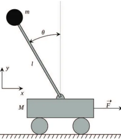
Fig. 1. Pendulum phenomenological model.
interested so much in the time to swing-up the pendulum while their objective is its stabilization when it reaches its unstable equilibrium point. This paper describes a method to swing-up a pendulum attached to a cart in a minimum time with a control in open-loop form. The necessary condition derives from the Pontryagin Maximum Principle and yields that the optimal time control has a bang-bang structure. Unfortunately, the use of shooting method based on the indirect method does not give any satisfactory results because of the hardness of the non-linear dynamics of the system. We focus then on the discretization method to provide us an approached solution. This last solution will be used to be reÞned via a Þnishing procedure by taking into account the structure of the control. In Section 2, the differential equations which come from the IP system are presented yielding the optimal time control problem that we have to solve. In section 3, we deduce the structure of the optimal time control by applying the necessary condition of the PMP. By discretizing the optimal control problem, we propose in Section 4 a method to reÞne the solution obtained, and some numerical simulations are performed. In Section 5, we conclude.
II. INVERTEDPENDULUM MODEL
Mathematical models of mechanical systems are usually described by Hamiltonian or Euler-Lagrange equations.
In Þgure 1, a model of the IP systems is displayed. The model used in this paper consists in two rods symmetrically hinged to a cart which can move horizontally by means of horizontal forces, driven by DC motor which is the control of the system. The cart is able to move on a limited horizontal rail with length |Lr| ≤ 0.5m, and the force of the DC motor
on the cart is denoted by F . The system has one input and four outputs. The outputs are: (i) the cart horizontal distance x in relation to the center of the track ; (ii) the angular poles θ from the downward equilibrium point ; (iii) cart velocity ˙x and (iv) pendulum angular velocity ˙θ. The (control) input designated by u is the voltage Vm that drives the DC motor.
Two points have to be kept in mind when the controllers are designed. The cart position and the control signal are both bounded in a real time application. The bound for the control signal is set to[−25V, 25V ] and the cart position is physically bounded by the rail length in the interval[−0.5m, 0.5m]. We consider in this model that θ = 0 is the stable position (the pendulum is below) and θ= ±π is the unstable position (the pendulum is on the top).
By applying the law of the dynamic on the inverted pen-dulum cart system, we get the following non-linear equations of motion:
(m + M )¨x+ b ˙x − mlcos(θ)¨θ+ mlsin(θ) ˙θ2= F, (1) −ml¨xcos(θ) + N ¨θ+ d ˙θ + mglsin(θ) = 0. (2) The system has several physical parameters associated with its components that are required for determining the differential equations. They are described in Table II. The values of these parameters are pulled from [1].
TABLE I. PENDULUM PARAMETERS.
Parameter SigniÞcance Value Km DC motor torque constant 0.05 N m
Kb Gearbox Gearing ratio 0.05 N/A
R Motor Armature Resistance 2.5 Ω r Motor pinion radius 0.0148 m
M Cart mass 2.4 kg
m Pendulum mass 0.23 kg
g Gravity 9.81 m/s2
l Pole length 0.36 m
N Moment of Inertia of the pole 0.099 kg.m2
b Cart friction coefÞcient 0.05 N s/rad d Pendulum damping coefÞcient 0.005 N ms/rad
The force that the DC motor provides on the cart is dependent on the input voltage u and on the velocity of the cart ˙x. The relationship is given by:
F = KmKb Rr u−
K2 mKb2
Rr2 ˙x . (3)
The state vector of the inverted pendulum-cart system is X = (x1, x2, x3, x4)t = (x, ˙x, θ, ˙θ)t, where x1 = x
is the cart position, x3 = θ represents the pendulum angle
(see Fig. 1), and x2= dxdt, x4 = dθdt are the velocity and the
angular velocity of the cart and the pendulum, respectively. From equations (1), (2) and (3), the dynamic equations of the inverted pendulum-cart system are given by:
˙ X = f (X) + b(X)u ⇔ ˙x1= x2 ˙x2= f1(X) + b1(X)u ˙x3= x4 ˙x4= f2(X) + b2(X)u where b1(X) = N KRrmh1(X) b2(X) = lmKmRrcos(θ)h1(X) f1(X) = h1(X)[h2(X) + h3(X) + h4(X)] f2(X) = h1(X)[h5(X) + h6(X)] and h1(X) = (N (M + m) − l2m2cos2(θ))−1 h2(X) = −(N KRrbK2m + N b) ˙x h3(X) = −gl2m2cos(θ)sin(θ) h4(X) = −dlm ˙θcos(θ) − N lm ˙θ2sin(θ) h5(X) = −(lmKRrb2Km+ blm) ˙xcos(θ) − dh ˙θ
h6(X) = −g(M + m)lmsin(θ) − l2m2˙θ2cos(θ)sin(θ)
The problem that we are interested in, can be formulated as an optimal time control problem in presence of state constraint on x1(t). We have to solve: min X(t),u(t) J(tf, X, u) = min Z tf 0 dt s.t. ˙ X= f (X) + b(X)u |x1(t)| ≤ 0.5 |u(t)| ≤ 25 (x1(0), x2(0), x3(0), x4(0)) = (0, 0, 0, 0) (x2(tf), x3(tf), x4(tf)) = (0, ± π, 0) (4)
III. THE USED SWING-UP CONTROLLER DESIGN Different control schemes were discussed to swing the pendulum from the downwards position to the upright position. One of these methods, namely heuristic controller, provides a constant voltage in the appropriate direction, and drives the cart along the track repeatedly. Thus, it will repeat this action until the pendulum is close enough to the upright position such that the stabilizing controller can be triggered to maintain this balanced state [1], [4].
Another scheme is an energy controller that regulates the amount of energy in the pendulum. This controller inputs energy into the cart-pendulum system until it attains the energy state that corresponds to the pendulum in the upright position. Similarly to the heuristic control method, the energy control method will also switch to the stabilizing controller when the pendulum is close to the upright position.
The switch that triggers the stabilizing controller in both cases is activated when the pendulum is within0.1 radians of the upright position and the angular velocity is slower than2.5 radians per second [2], [6], [8].
Although the swing-up controllers described above are on the feedback form, the objective in this work is to swing-up the pendulum from the downward position θ= 0 to the upright one θ= ±π in minimum time with an open-loop form.
IV. INDIRECT METHOD USINGPMP
In this case, we consider the Problem (4) and we relaxe the state constraint|x1(t)| ≤ ∞. One can understand that we
can solve the relaxed problem as considering the rail is long enough, but this constraint could be restored after resolving the problem by replacing the cart at the beginning in the adequate
position in order to satisfy this constraint. From the PMP, we deduce the expression of the optimal time control of Problem (4), which has a bang-bang structure. Indeed, we introduce the adjoint states variables p(t) = (p1(t), p2(t), p3(t), p4(t)),
and we deÞne the Hamiltonian function as:
H(t, X, p, u) = p0+ p1x2+ p2(f1(X) + b1(X)u) + p3x4+
p4(f2(X) + b2(X)u),
which is linear in relation with u. With p0 = −1 (maximum
principle), the adjoint states variables verify the equations ˙p = −∂H(t,X,p,u)∂X and are given by
˙p1= −∂x∂H1 = 0 ˙p2= −∂x∂H2 = −p1− p2( ∂f1(X) ∂x2 + ∂b1(X) ∂x2 u) −p4(∂f∂x2(X)2 + ∂b2(X) ∂x2 u) ˙p3= −∂x∂H3 = −p2( ∂f1(X) ∂x3 + ∂b1(X) ∂x3 u) −p4(∂f∂x2(X)3 + ∂b2(X) ∂x3 u) ˙p4= −∂x∂H4 = −p2( ∂f1(X) ∂x4 + ∂b1(X) ∂x4 u) − p3 −p4(∂f∂x2(X)4 + ∂b2(X) ∂x4 u) (5)
The maximum of the Hamiltonian H leads to the optimal control which has a bang-bang structure:
u(t) = Vmaxsign(p2b1(X) + p4b2(X)) (6)
where Vmax= 25V is the maximum voltage delivered by the
DC motor.
The classical approach based on the PMP (indirect method), known for its speed and accuracy, has been tested on this optimization problem. However, its implementation using shooting techniques may (in practice) deal with some difÞculties. Indeed, the shooting method consists to Þnd a zero of the shooting function S(y) = ˆz(tf) − (0, ± π, 0), where
ˆ
z corresponds to the integration of the Initial Value Problem (IVP) associated with the original problem
(IV P ) ˙ X= f (X) + b(X)u ˙p = −∂H(t,X,p,u)∂X X(0) = 0 p(0) = y. (7)
After applying necessary conditions of optimality, this method has to solve a system of non-linear differential equations. However, its main drawback is the need of a correct starting point: as this method typically involve applying a quasi-Newton based algorithm using the shooting function, the radius of convergence can be very low, depending on the regularity of the problem. The shooting method does not converge systematically, and one understands that it is not realistic to hope to solve the relaxed Problem (4) by this way.
V. DIRECT METHOD USING DISCRETIZATION TECHNIQUES Considering direct methods which traditionally involve total or partial discretizations of the problem, we have to use various local approaches to solve the arising optimization problem. These methods are generally imprecise and they can lead to the resolution of large scale problems depending on the used step of discretization.
At the heart of a well-founded discretization method for solving optimal control problems, one has the following three
0 0.5 1 1.5 2 í5 0 5 Cart"s Velocity 0 0.5 1 1.5 2 í0.5 0 0.5 Cart"s Position 0 0.5 1 1.5 2 í10 0 10
Pendulum"s Angular Velocity
0 0.5 1 1.5 2 í5 0 5 Pendulum"s Angle 0 0.5 1 1.5 2 í50 0 50 Control
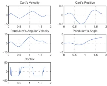
Fig. 2. Simulation of Swing-up control in optimal time.
fundamental components: - methods for solving the differential equations and integrating functions ; - a method for solving a system of non-linear algebraic equations ; and - a method for solving a non-linear optimization problem.
Methods for solving differential equations and integrating functions are required for all numerical methods in optimal control. In a direct method, the numerical solution of differ-ential equations is combined with non-linear optimization. In this work, the time-marching is the considered approach used for solving the differential equations with an explicit fourth order Runge-Kutta integrator.
In a direct method, the state and the control are discretized in some manner and the problem is transcribed to a non-linear programming problem (NLP). The NLP is then solved using well-known optimization techniques (we use the fmincon MatLab subroutine). In a direct method, the optimal solution is found by transcribing an inÞnite-dimensional optimization problem into a Þnite-dimensional one. In Figure 2, the obtained solution is drawn, and one remarks that the optimal time con-trol is not a bang-bang concon-trol but possesses a structure close to a switching function. This structure will be exploited from the approximated switching times and a Þnishing procedure is implemented. Note that the corresponding minimum time is about 1.79 seconds.
A. Finishing procedure
A system of non-linear algebraic equations can be consid-ered equivalently to root-Þnding one. In this case, where all of the algebraic equations can be written as equalities, we have a problem of the form S(y) = 0. The most common method for solving a multidimensional root-Þnding problem is a Newton based method, and an initial point is made of the vector y. It is well-known that the Newton method converges when the initial point is close to a root.
The Þnishing procedure consists in constructing the solu-tion of the system of non-linear equasolu-tions. Then the system
0 0.5 1 1.5 2 í5 0 5 Cart"s Velocity 0 0.5 1 1.5 2 í1 0 1 Cart"s Position 0 0.5 1 1.5 2 í10 0 10
Pendulum"s Angular Velocity
0 0.5 1 1.5 2 í5 0 5 Pendulum"s Angle 0 0.5 1 1.5 2 í50 0 50 Control u*(t)
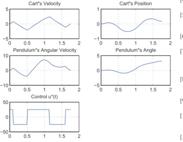
Fig. 3. Solution adjusted by the Þnishing procedure.
is solved using a Newton based method with the initial approximation which is uniquely determined from the switch times of the problem obtained at the end of the algorithm which solve a non-linear optimization problem (7). According to Newton based method, the switching function (bang-bang control) is constructed using the fsolve MatLab subroutine. The optimal time control u∗(t) corresponding to the switching
function is drawn in Figure 3 and the minimum time is about 1.75 seconds.
VI. CONCLUSION
This study presents the simulation and the results of an optimal time control problem which deals with the balancing of a cart inverted pendulum driven by a motor. By using tools from optimal control theory through the PMP, we have obtained a description of the optimal time control problem, for the problem with the voltage of the DC motor as control inputs. In order to determine the solution, we used the direct method based on the discretization techniques and the computations are performed using fmincon from MatLab. From the bang-bang structure of the optimal control, the Þnishing procedure based on the switching times is used. It operates with a Newton based method. This approach appears to work efÞciently very well for the resolution of the system studied here. Further study on this system would bring signiÞcant beneÞts to robotic and control professional.
REFERENCES
[1] R. Mellah, F. Lahouazi, S. Djennoune, S. Guermah and R. Toumi,
Composite Sliding Mode Control of Inverted Pendulum, International
Journal of Control, Automation and Systems, Vol. 1, No. 3, May 2012. [2] W. Zhong and H. Rock, Energy and Passivity Based Control of the
Double Inverted Pendulum on a Cart, Proceedings of the 2001 IEEE
International Conference on Control Applications, September 5-7, Mex-ico City, 2001.
[3] A. Bogdanov, Optimal Control of a Double Inverted Pendulum on
the Cart, Technical Report CSE-04-006, OGI School of Science and
Engineering, OHSU, 2004
[4] M. Bugeja, Non-Linear Swing-Up and Stabilizing Control of an Inverted
Pendulum system, University of Malta, Msida, Malta, 2002.
[5] C. A. Ibanez, O. Gutierrez Frias and M. Suarez Castanon,
Lyapunov-Based Controller for the Inverted Pendulum Cart System, Nonlinear
Dynamics 40: 367374, Springer 2005.
[6] K. J. Astrom and K. Furuta, Swinging Up a Pendulum by Energy Control, Automatica, vol. 36, no. 2, pp. 287-295, February 2000.
[7] W. Zhong, Yang Chen and Fang, Minimum-Time Swing-up of a Rotary
Inverted Pendulum by Iterative Impulsive Control, Proceeding of the 2004
American Control Conference, June 30-July 2, Boston, pp:1335-1340, 2004.
[8] N. Muskinja and B. Tovornik, Swinging Up and Stabilization of a Real
Inverted Pendulum, IEEE Transactions on Industrial Electronics, Vol. 53,
No. 2, pp:631-639, 2006.
[9] F.L. Chernousko, S.A. Reshmin, Time-optimal swing-up feedback control
of a pendulum, Nonlinear Dyn., Vol 47, pp. 65-73, 2007.
[10] P. Mason, M. Broucke and B. Piccoli, Time Optimal Swing-Up of the
Planar Pendulum, IEEE Transactions on Automatic Control, Vol. 53, No.
8, pp. 1876-1886, 2008.
[11] P. Melba Mary and N. S. Marimuthu, Minimum Time Swing Up and
Stabilization of Rotary Inverted Pendulum Using Pulse Step Control,
Iranian Journal of Fuzzy Systems Vol. 6, No. 3, pp. 1-15, 2009. [12] V. Sukontanakarn and M. Parnichkun, Real-Time Optimal Control for
Rotary Inverted Pendulum, American Journal of Applied Sciences 6 (6):