To link to this article : DOI :
10.1109/TITS.2015.2437452
URL :
http://dx.doi.org/10.1109/TITS.2015.2437452
To cite this version :
Alligier, Richard and Gianazza, David and Durand,
Nicolas Machine Learning and Mass Estimation Methods for Ground-Based
Aircraft Climb Prediction. (2015) IEEE Transactions on Intelligent
Transportation Systems, vol. 16 (n° 6). pp. 3138-3149. ISSN 1524-9050
O
pen
A
rchive
T
OULOUSE
A
rchive
O
uverte (
OATAO
)
OATAO is an open access repository that collects the work of Toulouse researchers and
makes it freely available over the web where possible.
This is an author-deposited version published in :
http://oatao.univ-toulouse.fr/
Eprints ID : 16842
Any correspondence concerning this service should be sent to the repository
administrator:
[email protected]
Machine Learning and Mass Estimation Methods
for Ground-Based Aircraft Climb Prediction
Richard Alligier, David Gianazza, and Nicolas Durand
Abstract—In this paper, we apply machine learning meth-ods to improve the aircraft climb prediction in the context of ground-based applications. Mass is a key parameter for climb prediction. As it is considered a competitive parameter by many airlines, it is currently not available to ground-based trajectory predictors. Consequently, most predictors today use a reference mass that may be different from the actual aircraft mass. In previous papers, we have introduced a least squares method to estimate the mass from past trajectory points, using the physical model of the aircraft. Another mass estimation method, based on an adaptive mechanism, has also been proposed by Schultz et al. We now introduce a new approach, in which the mass is considered the response variable of a prediction model that is learned from a set of example trajectories. This machine learning approach is compared with the results obtained when using the base of aircraft data (BADA) reference mass or the two state-of-the-art mass estimation methods. In these experiments, nine different aircraft types are considered. When compared with the baseline method (respectively, the mass estimation methods), the Machine Learning approach reduces the RMSE (Root Mean Square Error) on the predicted altitude by at least 58% (resp. 27%) when assuming the speed profile to be known, and by at least 29% (resp. 17%) when using the BADA speed profile except for the aircraft types E145 and F100. For these types, the observed speed profile is far from the BADA speed profile.
Index Terms—Aircraft trajectory prediction, mass estimation, base of aircraft data (BADA), machine learning.
I. INTRODUCTION
A
IRCRAFT trajectory prediction has always been a key issue for many on-board and ground-based applications in Air Transportation. It is even more true since the current Air Traffic Management and Control (ATM/ATC) system is shifting towards trajectory-based operations within the framework of the European SESAR program [1] and its U.S. counterpart NextGen [2].As we are now in an era of global networks, where data flows between flying aircraft and ground-based control systems, one could think that ground-based trajectory prediction is no longer necessary: accurate on-board trajectory predictions could be
The authors are with Ecole Nationale de l’Aviation Civile, Laboratoire de Mathématiques Appliquées, Informatique et Automatique pour l’Aérien (MAIAA), 31055 Toulouse, France, and also with Institut de Recherche en Informatique de Toulouse/Algorithmes Parallèles et Optimisation (IRIT/APO), Université de Toulouse, F-31400 Toulouse, France (e-mail: richard.alligier@ enac.fr).
Color versions of one or more of the figures in this paper are available online at http://ieeexplore.ieee.org.
Digital Object Identifier 10.1109/TITS.2015.2437452
downloaded directly to the ground systems. Although this last statement is actually true, we are still in great need of accurate ground-based trajectory predictors. Some of the most recent algorithms designed to solve ATM/ATC problems do require testing a large number of alternative trajectories and it would be impractical to download them all from the aircraft. As an exam-ple of such algorithms, in [3] an iterative quasi-Newton method is used to find trajectories for departing aircraft, minimizing the noise annoyance. Another example is [4] where Monte Carlo simulations are used to estimate the risk of conflict between trajectories in a stochastic environment. Some of the automated tools currently being developed for ATM/ATC can detect and solve conflicts between trajectories (see [5] for a review). These algorithms may use Mixed Integer Programming [6], Genetic Algorithms [7], [8], Ant Colonies [9], or Differential Evolution or Particle Swarm Optimization [10] to find optimal solutions to air traffic conflicts.
To be efficient, all these methods require a fast and accurate trajectory prediction, and the capability to test a large number of “what-if” trajectories. Such requirements forbid the sole use of on-board trajectory prediction, which is certainly the most accu-rate, but is not sufficient for these most promising applications. Most trajectory predictors rely on a point-mass model to de-scribe the aircraft dynamics. The aircraft is simply modeled as a point with a mass, and the second Newton’s law is applied to relate the forces acting on the aircraft to the inertial acceleration of its center of mass. Such a model is formulated as a set of differential algebraic equations that must be integrated over a time interval in order to predict the successive aircraft positions, knowing the aircraft initial state (mass, current thrust setting, position, velocity, bank angle, etc.), atmospheric conditions (wind, temperature), and aircraft intent (thrust profile, speed profile, route).
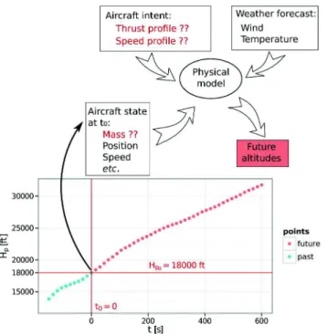
Unfortunately, the data that is currently available to ground-based systems for trajectory prediction purposes is of fairly poor quality. The speed intent and aircraft mass, being consid-ered competitive parameters by many airline operators, are not transmitted to ground systems. The actual thrust setting of the engines (nominal, reduced, or other, depending on the throttle’s position) is unknown. There are uncertainties or noise in the Weather and Radar data. The problem of unknown parameters such as the mass, thrust law, and target speeds, is of particular importance when predicting the aircraft climb. Fig. 1 illustrates the climb prediction problem, when using a physical model of the aircraft dynamics.
Some studies [11]–[13] detail the potential benefits that would be provided by additional or more accurate input data. In other works, the aircraft intent is formalized through the
Fig. 1. The ground-based aircraft climb prediction problem.
definition of an Aircraft Intent Description Language [14], [15] that could be used in air-ground data links to transmit some useful data to ground-based applications. All the necessary data required to predict aircraft trajectories might become available to ground systems someday. In the meantime, we propose to learn some of the unknown parameters of the point-mass model from the data that is already available today, typically from the observed radar tracks of past and current flights.
In this paper, we apply Machine Learning techniques to learn the aircraft mass. We show how our method improves the climb prediction when compared with the baseline method (see Fig. 2) that uses the reference mass from the Eurocontrol Base of Aircraft Data (BADA). We also compare our Machine Learning approach to two other mass estimation methods [16], [17] that rely solely on the physical model of the aircraft dynamics to estimate the mass from the past trajectory points.
The rest of this paper is organized as follows: Section I gives some background on the estimation of aircraft model param-eters and highlights the differences between mass prediction (using Machine Learning) as we introduce it in this paper, and mass estimation (using the physical model). Section II details the data used in this study. Section III presents some useful Machine Learning notions that help understanding the methodology applied in our work. The application of Machine Learning techniques to our mass prediction problem is de-scribed in Section IV, and the results are shown and discussed in Section V, before the conclusion.
II. BACKGROUND, MASSPREDICTION VS. ESTIMATION
A. Estimation of Physical Model Parameters
Focusing on the aircraft climb, and considering a physical model of the aircraft dynamics, we are interested in this paper in estimating some key parameters for climb performance using the past trajectory points. This approach, where some unknown
Fig. 2. Baseline method: the BADA prediction of the future aircraft climb.
parameters are adjusted by fitting the model to the observed past trajectory, is not new. The past publications following this path [17]–[24] propose several methods, with different choices for the adjusted parameter (mass, or thrust, for example), the modeled variable that is fitted on past observations (rate of climb, energy rate), and the algorithm that is applied (stochastic method, adaptive mechanism, least squares, etc).
In [21] Lymperopoulos, Lygeros, and Lecchini model the aircraft mass and the wind encountered during climb as sources of uncertainty. These stochastic variables are sampled from chosen distributions to produce random simulated trajectories. Each trajectory is then weighted according to its probability to give the aircraft positions measured just after takeoff. The uncertainty on the future aircraft positions is reduced by se-lecting the parameters of highest probability after a number of measurements. The method is tested in a simulation en-vironment. In [20], Slater introduces an adaptive mechanism improving the trajectory prediction by dynamically adjusting the modeled thrust. The aircraft mass is assumed to be equal to a standard reference mass for the chosen aircraft type. The results presented in [20] show significant improvements in the climb prediction accuracy for simulated data, and much fewer improvements when applied to a few examples using real trajectories. Other works propose to adjust the mass instead of the thrust.
Among the publications dealing with mass estimation, let us cite [18], where Warren and Ebrahimi propose an equivalent
weight as a workaround to use a point-mass model without knowing the actual aircraft mass. Nominal thrust and drag profiles are assumed. The equivalent mass is found by mini-mizing the gap between the computed and observed vertical rates. A second study [19] raises doubts about the reliability of the vertical rate for this purpose, and suggests to use the energy rate instead. The proposed method is tested on simulated trajectories only. In more recent works, Schultz, Thipphavong,
Fig. 3. Mass estimation (left) vs. mass prediction (right).
and Erzberger [17] introduce an adaptive mechanism where the modeled mass is adjusted by fitting the modeled energy rate with the observed energy rate. This adaptive method provides good results on simulated traffic and this method has also been successfully applied on actual radar data [25], [26].
In [22], [23], we use a Quasi-Newton algorithm (BFGS) combined to a mass estimation method to learn the thrust profile minimizing the error between the modeled and observed energy rate. This method has been tested on two months of real data, showing good results. Concerning the mass estimation method, we showed that, when using the BADA1model of the
forces (or a similar model), the aircraft mass can be estimated at any past point of the trajectory by solving a polynomial equation, knowing the thrust setting at this point. When using several points, and assuming a constant mass over the whole trajectory segment, the mass can be estimated by minimizing the quadratic error on the energy rate. In our latest papers [16], [27], we introduce a variant of this mass estimation method, taking the fuel burn into account, and compare it with the adaptive method of Schultz et al.. In the current paper, we propose a completely different approach, where the aircraft mass is predicted by a model learned from examples.
B. Mass Prediction vs. Mass Estimation
Both the adaptive [25] and least square [22], [23] methods evoked in previous Section I-A rely solely on the physical model to estimate the mass from past trajectory points. The mass is adjusted so that the modeled power fits the energy rate observed on the past points, assuming the thrust profile to be known. This mass estimation approach is illustrated on the left part of Fig. 3.
1BADA: the Eurocontrol Base of Aircraft Data.
The Machine Learning approach we introduce in this paper makes use of additional data found in a database of trajectory examples. The idea is to learn a prediction model from the examples, as illustrated on the right part of Fig. 3. Instead of directly adjusting the mass on the past trajectory points, we adjust a prediction model on a set of examples. Once the model is calibrated, it can be used to predict the mass on fresh trajec-tory inputs. The methodological issues concerning model selec-tion, parameter tuning, and performance assessment are briefly presented in Section III. For now, let us just say that, in the Machine Learning approach, a set of examples(yi, xi)16i6n
is used to build a model which relates the predicted variable y to some explanatory variables x. In our case, the predicted variabley is the aircraft mass m. Unfortunately—and this is the crux of our problem—the actual mass is not available in our data.
In order to build examples that can be used by Machine Learning algorithms, we propose, for each example trajectory, to adjust a modeled mass so that the modeled power fits the observed energy rate as best as possible on the “future” points. Here, the terms “past” and “future” refer to the fact that the aircraft altitude is respectively below or above a reference pres-sure altitudeHp0, assuming we want to predict the successive
altitudes aboveHp0when the climbing aircraft crosses altitude
Hp0. The modeled mass is adjusted using the least square
method introduced in [22], [23].
In other words, we propose to replace the actual massm, missing in our data, by an adjusted mass mˆfuture that gives
the best possible fit of the energy rate on our examples, assuming a max climb thrust setting. This mass mˆfuture is
the y output variable of the prediction model learned by the Machine Learning methods. The explanatory variablesx, are computed from the “past” data that is available when the aircraft crossesHp0.
The Radar and Weather data, as well as the construction of our examples, are described in more details in Section II.
C. Applying Our Method in Actual Operations
The proposed method consists in learning a model that can predict the aircraft mass, given Radar and Weather data inputs, or any other relevant additional inputs (e.g. flight plan). This model is learned on a data set of example trajectories. Once learned, it can be used for predicting the aircraft mass on fresh input trajectories. The predicted mass can then be used as input to the physics-based model that is already used in operations, in order to produce an accurate trajectory prediction.
When applying such a Machine Learning method in opera-tions, one must first collect trajectory data, build a training set, and tune the model. This should be done for every aircraft type for which there is sufficient training data. Tuning one model per aircraft is no more an issue than for the standard BADA model, for which there is also one model per aircraft type or group of similar aircraft. Note however that, when using a Machine Learning approach, the performance of the tuned model highly depends on the quality of the collected data. For more accuracy, the training data sets should be specific to each airport or terminal area where we intend to apply our tuned model.
Note that in that respect, our approach is much easier to put in operations than purely data-driven methods as we still use the physics-based model. Purely data-driven approach relies on a statistical model to predict directly the altitude. This requires to tune a specific model for each mode of operation (e.g. climb at constant rate, or at constant calibrated airspeed, etc.). This means we need sufficient data for each aircraft type and each mode of operation, and for every airport where we intend to use such a model. In our case, we use the Machine Learning approach only to learn one of the input parameters—here the mass—of the physics-based model. This model is already in operation and remains valid whatever the chosen mode of oper-ation. Furthermore, for the aircraft types or airports for which there is not enough data of sufficient quality to learn a model predicting the mass, we can easily revert to the mass estimated solely from the past trajectory points, or to the reference BADA mass, while still using the physics-based model.
Airport and airline procedures might change over years, as well as the performances of the engines equipping the aircraft. These changes obviously impact the performance of the tuned model. To address this issue, one can monitor the model per-formance over time and tune it again when it becomes less performing.
III. DATAUSED INTHISSTUDY
A. Data Pre-Processing
Recorded radar tracks from Paris Air Traffic Control Center are used in this study. This raw data is made of one position report every 1 to 3 seconds, over two months (July 2006, and January 2007). In addition, the wind and temperature data from Météo France are available at various isobar altitudes over the same two months.
The raw Mode-C altitude2has a precision of 100 feet. Raw
trajectories are smoothed using splines. Basic trajectory data is made of the following fields: aircraft position (X, Y in a projec-tion plane, or latitude and longitude in WGS84), ground veloc-ity vectorVg= (Vx, Vy), smoothed altitude (Hp, in feet above
isobar 1013.25 hPa), rate of climb or descentdHp/dt. The wind
W = (Wx, Wy) and temperature T at every trajectory point
are interpolated from the weather data grid. The temperature differential∆T is computed at each point of the trajectory.
Using the position, velocity and wind data, we compute the true air speedVa. The successive velocity vectors allow us to
compute the trajectory curvature at each point. The aircraft bank angle is then derived from true airspeed and the curvature of the air trajectory.
Along with these variables derived from the Mode-C radar data and the weather data, we have access to some variables in the flight plan like the Requested Flight Level for instance.
With the weather data grid, we have also computed the temperature differential∆T (weather grid) and the wind along Walong(weather grid) at each altitude of the grid. This is done
by using theVaXY, the time, the latitude and the longitude of
the considered point.Walongis the wind along the true air speed
in the horizontal planeVaXY.
All the computed variables are summarized in Table I.
B. Filtering Climb Segments
Our data set comprises all flights departing from Paris-Orly (LFPO) or Paris-Charles de Gaulle Airport (LFPG). Needless to say, this approach can be replicated to other airports.
The trajectories are filtered so as to keep only the climb segments. An additional 80 seconds is clipped from the begin-ning and end of each segment so as to remove climb/cruise or cruise/climb transitions.
C. Building the Sets of Examples
The climb segments are sampled every 15 seconds. From these sampled segments, we build examples (or patterns) con-taining exactly 51 points. In these examples, the first 11 points (past trajectory) are used to predict the mass. The remaining points (future trajectory) are used to compute the error between the predicted and actual trajectory. In this study, we use two different datasets.
1) A Small A320 Data Set:In order to compare the different Machine Learning methods, we use a small set of examples notedA320small. This set of examples is built using climbing
segments of aircraft of type A320. The climbing segments are sampled in order to have the 11th point always3 at 18000 ft.
Thus, from one sampled climb segment, we build only one example. The resulting set of examples, denotedA320smallin
the following, contains 4939 examples. It is only used to choose a machine learning method.
2This altitude is directly derived from the air pressure measured by the aircraft. It is the height in feet above isobar 1013.25 hPa.
3Using the smoothed altitude Hp(t), we search for the t0 such that Hp(t0) = 18000 ft. Once this time is found, we sample 10 points before and 40 points after.
TABLE I
THISTABLESUMMARIZES THEVARIABLESAVAILABLE INOURSTUDY
2) A Larger Dataset With 9 Aircraft Types and Various Altitudes: This larger data set is used to compare the selected Machine Learning method to the baseline BADA predictor and to the two other methods using estimated masses (adaptive, or least squares), on 9 different aircraft types and with various altitudes for the “current” point.
The sampled climbing segments and the examples are built in a different way. The raw climb segments are smoothed and sampled every 15 seconds, starting at the first point. With each sampled climb segment, we build as much examples containing 51 successive points as we can. The 10 first points of each example are considered as the “past” points. The 11th point is the “current” point, and the next 40 points are the “future” points used to evaluate the prediction made using the 11 first points.
As a consequence, the 11th point is not always at 18000 ft. As we are mostly interested in altitude prediction in the
en-routeairspace, we only keep the patterns with the 11th point at an altitude above 15000 ft4for the B744 aircraft type and above 18000 ft for all the other aircraft types.
4The chosen minimum flight level for the Boeing 747-400 is lower than for the other aircraft types because we wanted to have enough examples in our data set.
TABLE II
SIZE OF THEDIFFERENTSETS. ONLY THECLIMBINGSEGMENTS
GENERATING ATLEASTONEEXAMPLE INOURFINALEXAMPLES
SETARECOUNTEDHERE. INOURDATA, NOFLIGHTHASMORE
THANONECLIMBINGSEGMENTGENERATINGEXAMPLES
The multiple examples extracted from a same trajectory might share many points. Consequently, when splitting our set into a training set and a test set, the results would be biased if we put some of these examples in the training set and the others in the test set. We have been very careful not to do that. The training and test sets are built by choosing randomly among the trajectories, not the examples they contain.
We have considered 9 aircraft types and we have built one examples data set for each aircraft type. Table II shows the size of the different data sets. The selected aircraft types are very different: for example, the E145 is a short haul aircraft with a 18500 kg reference mass while the B744 (Boeing 747-400) is a long haul aircraft with a 285700 kg reference mass.
D. Estimation of the Mass to be Predicted
The actual mass is not available in our radar data set. Thus, as explained in Section I-B, we have used the least square method proposed in [16] on the 41 future points of the trajectories. This method estimates a mass sequence corresponding to a sequence of trajectory points. This mass sequence takes into account the fuel consumption. It minimizes the sum of the squared differences between the observed specific energy rate and the computed specific power (see [16] for details).
Let us denotemˆ11,futurethe first mass of this sequence, that is
the mass at the “current” point (numbered 11 in our examples). This estimated massmˆ11,futureis the output variabley of the
prediction model we want to learn from examples. To estimate this mass for each of our example trajectories, we need to make some hypotheses concerning the thrust settings, which are not available in our data. We assume a standard BADA max climb thrust, during all climb.
As a consequence, the estimated mass might be quite dif-ferent from the actual one, especially for aircraft climbing at reduced power. This difference is not of crucial impor-tance, however, as there is an infinity of couples (mass,
thrust_profile) that give exactly the same trajectory. Intuitively, a heavy aircraft with maximum climb thrust is equivalent to a lighter aircraft with reduced thrust. Although it might not be realistic, the modeled mass can be adjusted so as to give an accurate prediction of the energy rate. Knowing the energy rate and the speed intent, one can predict the future altitudes of the aircraft.
TABLE III
STATISTICS,INFEET,ON THEDIFFERENCEBETWEEN THECOMPUTED ANDOBSERVEDALTITUDES(Hp(pred)( ˆm11,future) − Hp(obs))AT
DIFFERENTTIMERANGES FOR THEEXAMPLESSETA320small
E. Approximation of the Example Trajectories When Using the Estimated Massmˆ11,future
For verification purposes, let us assess the accuracy of the trajectory computed using the estimated mass on our set of examples. To do this, we compute the “future” trajectories using the speed profileVa = Va(obs)(t) and the mass ˆm11,future, and
observe the error in altitude.
Looking at Table III, we see that the differences between the predicted altitudes and the observed ones are limited.5 There remains an incompressible error, though, which might be due to the fact that some aircraft might not actually follow a constant
max climbthrust law, nor a constant reduced power climb. They might switch from one to the other during the climb. Learning the thrust settings is not the subject of the current paper, and has already been investigated in [23], and we shall assume a constant max climb thrust in the rest of this work.
Another possible source of error is the estimation of the true airspeedVa, which relies on the observed ground speed and the
wind forecast. Due to the uncertainties in the weather forecast, and the possible observation errors in the ground speed, the “observed” airspeed profile might lack accuracy.
In any case, Table III gives us an order of magnitude of the best possible approximation of the “future” trajectory that we can achieve with our data and assumptions, when using the estimated mass mˆ11,future. This approximation error is
computed on our set of examplesA320small, for verification
purposes. It is not representative of the prediction error that will be made when considering fresh trajectories.
Let us now see how we can apply Machine Learning methods to build a model that predictsmˆ11,future, and that will allow us
to predict new trajectories.
IV. MACHINELEARNING
This section presents some useful Machine Learning notions. We want to predict a variabley, here the aircraft mass m of a given trajectory, from a vector of explanatory variablesx, which in our case is the data extracted from the past trajectory points and the weather forecast. This is typically a regression problem. Naively said, we want to learn a functionf such that y = f (x) for all (x, y) drawn from the distribution (X, Y ). Actually, such a function does not exist, in general. For instance, if two ordered pairs(x, y1) and (x, y2) can be drawn with y16= y2,
f (x) cannot be equal to y1andy2at the same time.
A way to solve this issue is to use a real-valued loss function L. This function is defined by the user of the function f . The valueL(f (x), y) models a cost for the specific use of f when (x, y) is drawn. With this definition, the user wants a function
5Especially when compared with the first line of Table IX.
f minimizing the expected loss R(f ) defined by (1). The value R(f ) is also called the expected risk
R(f ) = E(X,Y )[L (f (X), Y )] . (1)
However, the main issue in order to choose a function f minimizingR(f ) is that we do not know the joint distribution (X, Y ). We only have a set of examples of this distribution.
A. Learning From Examples
Let us consider a set of n examples S = (xi, yi)16i6n
coming from independent draws of the same joint distribution (X, Y ). We can define the empirical risk Rempirical by the
equation below Rempirical(f, S) = 1 |S| X (x,y)∈S L (f (x), y) . (2)
Assuming that the values (L(f (x), y))(x,y)∈S are
indepen-dent draws from the same law with a finite mean and vari-ance, we can apply the law of large numbers giving us that Rempirical(f, S) converges to R(f ) as |S| approaches +∞.
Thereby, the empirical risk is closely related to the expected
risk. So, if we have to select f among a set of functions F minimizing R(f ), using a set of examples S, we select f minimizing Rempirical(f, S). This principle is called the
principle of empirical risk minimization.
Unfortunately, choosingf minimizing Rempirical(f, S) will
not always give usf minimizing R(f ). Actually, it depends on the “size”6 ofF and the number of examples |S| [29], [30].
The smaller isF and the larger is |S|, the more the principle of
empirical risk minimizationis relevant. When these conditions are not satisfied, the selectedf will probably have a high R(f ) despite a lowRempirical(f, S). In this case, the function f is
overfittingthe examplesS.
These general considerations above have practical conse-quences on the use of Machine Learning. Let us denote fS
the function in F minimizing Rempirical(., S). The expected
risk using fS is given by R(fS). We use the principle of
empirical risk minimization. As stated above, some conditions are required for this principle to be relevant. Concerning the size of the set of examplesS: the larger, the better. Concerning the size ofF , there is a tradeoff. The larger F is, the smaller min
f∈FR(f ) is. However, the larger F is, the larger the gap
betweenR(fS) and min
f∈FR(f ) becomes. This is often referred
to as the bias-variance tradeoff .
B. Accuracy Estimation
In this subsection, we want to estimate the accuracy obtained using a Machine Learning algorithmA. Let us denote A[T ]
6The “size” of F refers here to the complexity of the candidate models contained in F , and hence to their capability to adjust to complex data. As an example, if F is a set of polynomial functions, we can define the “size” of F as the highest degree of the functions contained in F . In classification problems, the “size” of F can be formalized as the Vapnik-Chervonenkis dimension.
the prediction model found by algorithmA when minimizing Rempirical(., S),7considering a set of examplesS.
The empirical risk Rempirical(A[S], S) is not a suitable
estimation ofR(A[S]): the law of large numbers does not apply here because the predictorA[S] is neither fixed nor independent from the set of examplesS.
One way to handle this is to split the set of examples S into two independent subsets: a training set ST and another
setSV that is used to estimate the expected risk ofA[ST], the
model learned on the training setST. For that purpose, one can
compute the holdout validation errorErrvalas defined by the
equation below
Errval(A, ST, SV) = Rempirical(A[ST], SV) . (3)
Cross-validation is an other popular method that can be used to estimate the expected risk obtained with a given learning algorithm. In a k-fold cross-validation method, the set of ex-amplesS is partitioned into k folds (Si)16i6k. Let us denote
S−i= S \ Si. In this method,k trainings are performed in order
to obtain the k predictors A[S−i]. The mean of the holdout
validation errors is computed, giving us the cross-validation estimation below CV (A, S) = k X i=1 |Si|
|S|Errval(A, S−i, Si). (4) This method is more computationally expensive than the holdout method but the cross-validation is more accurate than the holdout method [31]. In our experiments, the folds were stratified. This technique is said to give more accurate estimates [32].
The accuracy estimation has basically two purposes: i) model selection in which we select the “best” model using accuracy measurements and ii) model assessment in which we estimate the accuracy of the selected model. For model selection, the set SV inErrval(A, ST, SV) is called validation set whereas in
model assessment this set is called testing set.
C. Hyperparameter Tuning
Some learning algorithms have hyperparameters. These hy-perparameters λ are the parameters of the learning algorithm Aλ. These parameters cannot be adjusted using the empirical
risk because most of the hyperparameters are directly or indi-rectly related to the size ofF . Thus, if the empirical risk was used, the selected hyperparameters would always be the ones associated to the largestF .
These hyperparameters allow us to control the size of F in order to deal with the bias-variance tradeoff . These hyperpa-rameters can be tuned using the holdout method on a validation
setfor accuracy estimation. In order to findλ minimizing the accuracy estimation we have used a grid search which consists in an exhaustive search on a predefined set of hyperparameters. The algorithm 1 obtained is a learning algorithm without any hyperparameters. In this algorithm, 20% of the training set is held out as a validation set.
7Actually, depending on the nature of the minimization problem and cho-sen algorithm, this predictor A[S] might not be the global optimum for Rempirical(., S), especially if the underlying optimization problem is handled by local optimization methods.
Algorithm 1: Hyperparameters tuning for an algorithmAλ
and a set of examplesT (training set).
function TUNEGRID(Aλ,grid)[T ]
(TT, TV) ← split(80%,20%)(T ) λ∗← arg min λ∈grid Errval(Aλ, TT, TV) returnAλ∗[T ] end function
V. APPLYINGMACHINELEARNING TO OURPROBLEM
A. Different Sets of Variables
We want to findf such that ˆm11,future= f (x), with x the
information available when the prediction is computed. The choice of explanatory variablesx is of considerable importance to the performance of the prediction model.
In this work, the candidate explanatory variablesx are clas-sified in five groups of variables depending on their provenance and their type. These groups are described in Table IV. The r (“radar”) group contains 297 variables extracted from the available Radar data, for the 11 past points of each trajectory. Them (“mass”) group contains 3 numerical variables. Two ofˆ them are masses estimated using the adaptive [25] and least square [22], [23] methods.eLSis the root mean squared error
of the energy rate prediction obtained with the least square method on the past points of the trajectory. Thew (“weather”) group contains 20 numerical variables. This group contains∆T (weather grid) andWalong(weather grid) computed on the last
point of the past trajectory. These quantities are computed at the 10 different altitudes of the weather grid. Finally, thep (“flight plan”) group contains 3 numerical variables and groupc con-tains 3 categorical variables, also extracted from the flight plan. Several combinations of these groups are tested, as specified in Table IV:r, ˆmr, ˆmrw, ˆmprw and c ˆmprw. This last group contains categorical variables that can be handled straightfully by the Gradient Boosting Machine (GBM) algorithm, but not by the other Machine Learning methods that we used.
B. Machine Learning Algorithms
Five different classical Machine Learning algorithms were tested in this study. These algorithms optimize the risk given by a quadratic loss L(ˆy, y) = (ˆy − y)2. A multiple linear
re-gression on the k variables selected by a forward-selection MLR-FSk[33], [34], a Ridge regression Ridgeλ[35] withλ the
penalty hyperparameter, and a principal component regression PCRk[36] on thek principal components were tested. In these
three methods, the obtained model is a linear combination of the explanatory variables. However, the obtained models are different because these algorithms have different ways to control the set of functionsF through their hyperparameters. A single-layer neural network NNet(n,λ) [37] was tested with
a weight decayλ and a number of n hidden units. A stochastic gradient boosting tree algorithm GBM(m,J,ν) [38] was tested
TABLE IV
THISTABLESUMMARIZES THEDIFFERENTSETS OFVARIABLES
USED BY THEMACHINELEARNINGALGORITHMS
TABLE V
GRID OFHYPERPARAMETERSUSED INOUREXPERIMENTS
the shrinkage parameter. With this method the obtained model is a sum ofm regression trees. As opposed to the other methods, this method can easily handle categorical variables without any prior encoding. The hyperparameters grids for these algorithms are presented in Table V.
VI. RESULTS ANDDISCUSSION
All the statistics presented in this section are computed using a stratified 10-fold cross-validation embedding the hyperpa-rameter selection. Fig. 4 illustrates how the data is partitioned, denotingλ the hyperparameter vector. Our set of examples S is
Fig. 4. Cross-validation for model assessment, with an embedded holdout validation for hyperparameter tuning.
TABLE VI
STATISTICS,INPERCENTAGE,ON THERELATIVEERRORBETWEEN THEMASSCOMPUTED BY APREDICTIONMODEL AND THEMASS
ˆ
m11,futureADJUSTED FOREACHEXAMPLETRAJECTORY,
FOR THEDATASETA320small
partitioned in 10 folds(Si)16i610. The hyperparameters used
to learn fromS−i are selected using 20% of the foldS−i as a
validation set. The model learned with these hyperparameters onS−iis then used to predict the mass on the test setSi.
Ob-viously, the intersection of the training setS−iand the test set
Siis empty: they do not share any example. Overall, our set of
predicted values (masses or altitudes) is the concatenation of the ten TuneGrid(Aλ, grid)[S−i](Si) (see algorithm 1). Therefore,
all the statistics presented in this section are computed on test sets. Each large set of examplesS corresponding to one of the 9 aircraft types is split in 10 folds(Si)16i610, randomly choosing
the climb segments. Thus, all the examples generated by one climbing segment are only in one fold Si. This guarantees
that the examples in foldSiare independent from the ones in
S−i= S \ Si.
A. Prediction of the Massmˆ11,future
The results obtained with the Machine Learning algorithm on the set A320small are reported in Table VI. The results
obtained with the BADA reference massmref, as well as the
masses mˆLS and mˆAd estimated with the least square and
adaptive methods, are also stated in this table as a baseline. Looking at the 6th column showing the root mean squared
TABLE VII
STATISTICS,INPERCENTAGE,ON THERELATIVEERRORBETWEEN THEMASSCOMPUTED BY APREDICTIONMODEL AND THEMASS
ˆ
m11,futureADJUSTED FOREACHEXAMPLETRAJECTORY
error (RMSE), we can see that all linear models have about the same performance. Equally, NNet and GBM perform similarly, with a slight advantage for the latter. For all methods, the more variables we have, the more accurate the prediction is. However, the error on the mass is not significantly reduced by adding the group of variables w (“wind”) to the set ˆmr. The greater error reduction is obtained by adding the group m (“mass”)ˆ to the “radar” setr, especially for the linear models. This was expected, as these estimated masses are highly correlated with
ˆ
m11,future, with a correlation coefficient above 0.94. In
compar-ison, all the variables in setr have a correlation coefficient with ˆ
m11,futurebelow 0.61. However, one has to keep in mind that
these correlation coefficients are computed taking the variables one by one. In a regression context, all these variables are used altogether and as stated in [39]: variables that are useless by themselves can be useful together.
Among the different machine learning methods, the best results for theA320small data set are obtained with the GBM
method, with the variables c ˆmprw. Throughout the rest of the document we will use this setup (GBM withc ˆmprw) and compare it with the BADA baseline and the mass estimation methods, using the 9 large sets of examples.
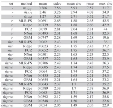
The results obtained for the larger data sets corresponding to 9 different aircraft types are presented in Table VII. When compared with the BADA reference mass method, the RMSE
TABLE VIII
STATISTICS,INFEET,ON THEDIFFERENCEBETWEEN THEPREDICTED ANDOBSERVEDALTITUDES(Hp(pred)( ˆm11) − H(obs)p )AT
TIMEt= 600S. THETRAJECTORIESARECOMPUTED
USING THESPEEDPROFILEVa= Va(obs)(t)
of the relative error on the mass is divided at least by 2 when using the GBM method. When compared with the two mass estimation methods, the RMSE of the relative error on the mass is reduced by at least 30% when using the GBM method.
B. Trajectory Prediction Using the Predicted Mass
In order to actually predict a trajectory using the BADA model and assuming a max climb thrust, one has to specify a mass, but also a speed profile. Both are usually unknown from ground systems. In our experiment, we want to evaluate the impact of the predicted mass on the trajectory prediction. Thus, we assume the speed profile to be known. The trajectory is computed using the mass predicted by the Machine Learning model and the speed profileVa = Va(obs)(t) observed on the
future points. With this setup, we just look at the influence of the predicted mass—and the energy rate prediction—on the altitude prediction, disregarding the additional errors that might be induced by erroneous assumptions on the speed intent.
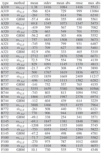
The results obtained on the trajectory prediction are pre-sented in Table VIII. The performance ranking of the methods is the same as in Table VII. This was to be expected, as both the computation of the response variable mˆ11,future in our
TABLE IX
THESESTATISTICS,INFEET,ARECOMPUTED ON THEDIFFERENCES
BETWEEN THEPREDICTEDALTITUDE AND THEOBSERVEDALTITUDE
(Hp(pred)( ˆm11) − Hp(obs))AT THETIMEt= 600 s. THETRAJECTORIES
ARECOMPUTEDUSING THEBADA SPEEDPROFILEVa= VaBADA
predicted mass rely on the same underlying physical model. Thus, an accurate mass prediction is likely to produce an accurate altitude prediction.
Using the GBM algorithm with the setc ˆmprw, the RMSE on the altitude at a 10 minutes look-ahead time is reduced by at least 58% when compared with the baseline obtained with the BADA reference massmref. When compared with the two
mass estimation methods, the RMSE is reduced by at least 28% when using the GBM method.
C. Results Using the BADA Speed Profile
In the previous subsection, we used the observed speed profileVa= Va(obs)(t) because we were interested in assessing
the errors related to a wrong mass prediction. However, in real life, this observed speed profile is not known when the predicted trajectory is computed. Thus, the results in Section V-B are not representative of what would be obtained in an operational context. For want of anything better one can use the speed profile specified in the BADA model.
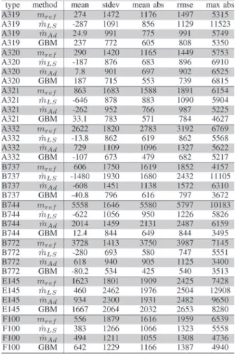
Using this BADA speed profile, Table IX presents the statis-tics on the error on the predicted altitude at timet = 600 s. Con-sidering the RMSE (6th column), we see that the performance ranking of the different methods is not as clear-cut as when the
speed profile is assumed to be perfectly known. However, for all aircraft types except E145, the Machine Learning approach using GBM still significantly improves the altitude prediction when compared with the baseline BADA method, with benefits ranging from 29% (F100) to about 85% (B772 and B744), in percentage. For the E145 type, we see that neither the GBM method nor the mass estimation methods improve the results.
When comparing GBM with the mass estimation methods, disregarding the E145 case, we see that GBM performs better, with a benefit of at least 17%, in all cases except for type F100 where the performances are similar.
The reason why the performance ranking of the different methods changes when taking the default BADA speed intent instead of the observed speed profile is quite simple. When in-vestigating our results, we found out huge differences between the actual speed profile and the BADA speed profile, especially for the aircraft types E145, F100, and B744. The root mean square of(Va(BADA)(Hp(obs)) − Va(obs)) for the aircraft E145,
F100 and B744 are respectively 76 kts, 42 kts and 36 kts while it is around 20 kts for the other aircraft types. The prediction for the B744 is still significantly improved when compared with the reference mass method because this reference mass is very different from the massmˆ11,future. For the two other
aircraft types for whichVa(BADA)is not in accordance with the
observed speedVa(obs), the benefit of learning or estimating the
mass is pretty much reduced, because of this poor estimation of the speed profile.
Note that if we focus on the 6 aircraft types for which the speed profile is relatively correct, the RMSE reduction ranges from 46% to 86% when comparing the Machine Learning approach with the BADA baseline, and from 17% to 49% when comparing with the mass estimation methods. In future work, the results might be improved by learning a model computing the future speed profile from the available variables.
D. Discussion on the Results
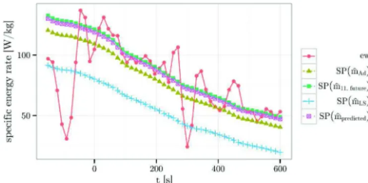
The mass estimation methods rely on a physical model (BADA) and the past trajectory points to compute the pre-diction. When making this prediction, we implicitly assume that the thrust law for the future points is the same as for the past points (e.g. max climb thrust all along the climb). This assumption might not always be true, however. The pilot may change the thrust settings during the climb for number of reasons: Air Traffic Control procedures or instructions, airline procedures, noise abatement, etc. Consequently, if our assump-tion on the future thrust setting is wrong, this will result in a wrong model of the specific power, as illustrated on Fig. 5. On this example, the observed energy rateewshows high variations
beforet = 0, and seems to stabilize at a higher level after t = 0. This is a typical case where the least square estimation method performs poorly: the modeled specific power (SP ( ˆmLS) on the
figure) is adjusted on the points beforet = 0, and gives a poor prediction aftert = 0. The adaptive method performs slightly better:SP ( ˆmAd) is closer to ewon the future points. This is
due to the adaptive mechanism limiting the influence of high variations of the observed energy rate.
Fig. 5. This figure portrays the computed specific power SP and the observed specific energy rate ew. Only one aircraft is considered here, however different masses are used to compute the specific power SP . According Newton’s law, the specific power SP of the aircraft is equal to the observed specific energy rate ew. The past points have a negative time.
On the example in Fig. 5, we see that the modeled power SP ( ˆmpredicted) using the predicted mass fits the observed
energy rate ew quite well on the points after t = 0. It is also
quite close toSP ( ˆm11,future), which is the best approximation
we can make when using the mass adjusted on the future points. In all methods, the mass is computed from the data that is available att = 0 i.e. at the moment when the trajectory predic-tion would be computed in an operapredic-tional context. However, the Machine Learning models make use of far more variables than the mass estimation methods. For instance, Machine Learning methods can use the distance between the departure and arrival airports as an explanatory variable. Such data is irrelevant in a physical model of the forces, though it does bring some information on the actual mass: the take-off weight of an aircraft depends on the fuel necessary to cross the distance to go. The Machine Learning approach can make use of such information, whereas the mass estimation methods cannot.
VII. CONCLUSION
To conclude, let us summarize our approach and findings, before giving a few perspectives on future works. In this study, we have tested Machine Learning methods using real Mode-C radar data. A model predicting the aircraft mass from a vector of explanatory variables is learned using Machine Learning techniques. This model is learned from a set of examples in which the response variable mˆ11,future is extracted from the
“future” points of each example trajectory.
We have compared our Machine Learning approach with the baseline Eurocontrol BADA (Base of Aircraft Data) method and with two state-of-the-art methods where the mass is esti-mated using the past trajectory points only. This comparison is made using a 10-fold cross-validation and for nine different aircraft types departing from the two main airports in Paris area. In a first step, we have assumed the “future” speed profile to be perfectly known so as to assess only the influence of the mass accuracy on the altitude prediction. When comparing our Machine Learning approach with the baseline, the RMSE on the predicted altitude is reduced by at least 58%, and up to nearly 92%, depending on the aircraft type. When comparing with the mass estimation methods, the RMSE reduction when using our method ranges from about 28% to 52%.
In a second step, we have used the default BADA speed profile so as to be as close as possible to the operational context where the actual speed intent is not known. In this context, the benefit of learning or estimating the mass is greatly reduced when the default BADA speed profile is far from the actual speed profile, which was the case for three aircraft types out of nine in our experimental setup. For the 6 remaining aircraft types, the reduction in RMSE on the altitude prediction ranges from 46% to 86% when comparing the Machine Learning approach with the BADA baseline, and from 17% to 49% when comparing with the mass estimation methods.
Concerning the 3 aircraft types (F100, E145, B744) for which the BADA speed profile poorly approximates the actual speed profile, the results still show a 85% reduction in RMSE for the B744 type when compared with the baseline, and a 28% reduction when comparing with the mass estimation methods. This is because the actual mass for this aircraft (Boeing 747-400) is also very poorly approximated by the BADA reference mass: Improving the mass prediction for such a heavy aircraft still does improve the altitude prediction, even when the speed profile is poorly estimated. For the F100 type (Fokker 100), the Machine Learning approach and the mass estimation methods give similar results, with a reduction in RMSE around 30%. Finally, there is only one aircraft type (E145) for which the poor BADA approximation of the speed profile cancels the benefits of learning or estimating the mass.
In future work, these results might be improved again by learning a model predicting the future speed profile from the explanatory variables.
From an operational point of view, the resulting improvement in the climb prediction accuracy would certainly benefit air traffic controllers, especially in the vertical separation task as shown in [17]. In future works, it could be interesting to test this method on Mode-S radar data which are more accurate than Mode-C radar data, and to extend our study to other airports.
REFERENCES
[1] SESAR Consortium, “Milestone deliverable D3: The ATM target con-cept,” Tech. Rep., 2007.
[2] H. Swenson, R. Barhydt, and M. Landis, “Next generation air transporta-tion system (NGATS) air traffic management (ATM)-Airspace project,” Nat. Aeron. Space Admin., Greenbelt, MD, USA, Tech Rep., 2006. [3] X. Prats, V. Puig, J. Quevedo, and F. Nejjari, “Multi-objective optimisation
for aircraft departure trajectories minimising noise annoyance,” Transp.
Res. C, Emerging Technol., vol. 18, no. 6, pp. 975–989, Dec. 2010. [4] G. Chaloulos, E. Crück, and J. Lygeros, “A simulation based study of
subliminal control for air traffic management,” Transp. Res. C, Emerging
Technol., vol. 18, no. 6, pp. 963–974, Dec. 2010.
[5] J. K. Kuchar and L. C. Yang, “A review of conflict detection and reso-lution modeling methods. IEEE Trans. Intell. Transp. Syst., vol. 1, no. 4, pp. 179–189, Dec. 2000.
[6] L. Pallottino, E. M. Feron, and A. Bicchi, “Conflict resolution prob-lems for air traffic management systems solved with mixed integer pro-gramming,” IEEE Trans. Intell. Transp. Syst., vol. 3, no. 1, pp. 3–11, Mar. 2002.
[7] J. M. Alliot, H. Gruber, and M. Schoenauer, “Genetic algorithms for solving ATC conflicts,” in Proc. 9th Conf. Artif. Intell. Appl., 1992, pp. 338–344.
[8] N. Durand, J. M. Alliot, and J. Noailles, “Automatic aircraft conflict resolution using genetic algorithms,” in Proc. Symp. Appl. Comput., Philadelphia, PA, USA, 1996, pp. 289–298.
[9] N. Durand and J.-M. Alliot, “Ant colony optimization for air traffic conflict resolution,” in Proc. 8th USA/Europe Air Traffic Manage. Res.
[10] C. Vanaret, D. Gianazza, N. Durand, and J. B. Gotteland, “Benchmark for conflict resolution (regular paper),” in Proc. ICRAT, Berkeley, CA, USA, May 2012, pp 1–8. [Online]. Available: http://www.icrat.org
[11] G. Mykoniatis and P. Martin, “Study of the acquisition of data from air-craft operators to aid trajectory prediction calculation,” EUROCONTROL Experimental Center, Brétigny-sur-Orge, France, Tech. Rep., 1998. [12] ADAPT2, Aircraft data aiming at predicting the trajectory. Data
anal-ysis report, EUROCONTROL Experimental Center, Brétigny-sur-Orge, France, Tech. Rep., 2009.
[13] R. A. Coppenbarger, “Climb trajectory prediction enhancement using airline flight-planning information,” in Proc. AIAA Guid., Navig., Control
Conf., 1999, pp. 1–11.
[14] J. Lopez-Leones, M. A. Vilaplana, E. Gallo, F. A. Navarro, and C. Querejeta, “The aircraft intent description language: A key enabler for airground synchronization in trajectory-based operations,” in Proc. 26th
IEEE/AIAA DASC, 2007, pp. 1.D.4-1–1.D.4-12.
[15] J. Lopes-Leonés, “The aircraft intent description language,” Ph.D. disser-tation, Dept. Aerospace Sci., Univ. Glasgow, Glasgow, U.K., 2007. [16] R. Alligier, D. Gianazza, and N. Durand, “Ground-based estimation of
air-craft mass, adaptive vs. least squares method,” in Proc. 10th USA/Europe
Air Traffic Manage. Res. Develop. Semin., 2013, pp. 1–10.
[17] C. Schultz, D. Thipphavong, and H. Erzberger, “Adaptive trajectory pre-diction algorithm for climbing flights,” in Proc. AIAA GNC, Aug. 2012, pp. 1–16.
[18] A. W. Warren and Y. S. Ebrahimi, “Vertical path trajectory prediction for next generation ATM,” in Proc. 17th AIAA/IEEE/SAE DASC, Oct. 31– Nov. 7, 1998, vol. 2, pp. F11/1–F11/8.
[19] A. W. Warren, “Trajectory prediction concepts for next generation air traf-fic management,” in Proc. 3rd USA/Europe ATM R D Semin., Jun. 2000, pp. 1–10.
[20] G. L. Slater, “Adaptive improvement of aircraft climb performance for air traffic control applications,” in Proc. IEEE Int. Symp. Intell. Control, Oct. 2002, pp. 602–607.
[21] I. Lymperopoulos, J. Lygeros, and A. Lecchini Visintini, “Model based aircraft trajectory prediction during takeoff,” in Proc. AIAA Guid., Navig.
Control Conf. Exhib., Keystone, CO, USA, Aug. 2006, pp 1–12. [22] R. Alligier, D. Gianazza, and N. Durand, “Energy rate prediction using
an equivalent thrust setting profile (regular paper),” in Proc. ICRAT, Berkeley, CA, USA, May 2012, pp 1–7. [Online]. Available: http://www. icrat.org
[23] R. Alligier, D. Gianazza, and N. Durand, “Learning the aircraft mass and thrust to improve the ground-based trajectory prediction of climbing flights,” Transp. Res. C, Emerging Technol., vol. 36, pp. 45–60, Nov. 2013. [24] A. Hadjaz, G. Marceau, P. Savéant, and M. Schoenauer, “Online learning for ground trajectory prediction,” in Proc. SESAR Innov. Days
EUROCONTROL, 2012, pp. 1–17.
[25] D. P. Thipphavong, C. A. Schultz, A. G. Lee, and S. H. Chan, “Adaptive algorithm to improve trajectory prediction accuracy of climbing aircraft,”
J. Guid. Control Dyn., vol. 36, no. 1, pp. 15–24, 2012.
[26] Y. S. Park and D. P. Thipphavong, “Performance of an adaptive trajectory prediction algorithm for climbing aircraft,” in Proc. Aviation Technol.,
Integr., Oper. Conf., Aug. 8, 2013, pp. 1–14.
[27] R. Alligier, D. Gianazza, M. G. Hamed, and N. Durand, “Comparison of two ground-based mass estimation methods on real data (regular paper),” in Proc. ICRAT, Istanbul, Turkey, May 2014, pp 1–8. [Online]. Available: http://www.icrat.org
[28] A. Nuic, User Manual for Base of Aircarft Data (Bada) Rev.3.9, Brussels, Belgium: EUROCONTROL, 2011, Tech. Rep.
[29] V. N. Vapnik and A. Y. Chervonenkis, “The necessary and sufficient conditions for consistency of the method of empirical risk minimization,”
Pattern Recognit. Image Anal., vol. 1, no. 3, pp. 284–305, 1991. [30] V. N. Vapnik, The Nature of Statistical Learning Theory. New York, NY,
USA, Springer-Verlag, 1995.
[31] A. Blum, A. Kalai, and J. Langford, “Beating the hold-out: Bounds for k-fold and progressive cross-validation,” in Proc. 12th Annu. Conf.
Comput. Learn. Theory, 1999, pp. 203–208.
[32] R. Kohavi, A Study of Cross-Validation and Bootstrap for Accuracy
Esti-mation and Model Selection. San Mateo, CA, USA: Morgan Kaufmann, 1995, pp. 1137–1143.
[33] C. R. Rao and H. Toutenburg, Linear Models: Least Squares and
Alterna-tives (Springer Series in Statistics). Berlin, Germany: Springer-Verlag, Jul. 1999.
[34] A. Miller, Subset Selection in Regression. Boca Raton, FL, USA: CRC Press, 2002.
[35] A. E. Hoerl and R. W. Kennard, “Ridge regression: Biased estimation for nonorthogonal problems,” Technometrics, vol. 12, no. 1, pp. 55–67, Feb. 1970.
[36] I. T. Jolliffe, “A note on the use of principal components in regression,”
J. R. Stat. Soc. Ser. C, Appl. Stat., vol. 31, no. 3, pp. 300–303, 1982. [37] B. D. Ripley, Pattern Recognition and Neural Networks. Cambridge,
U.K.: Cambridge Univ. Press, 2007.
[38] J. H. Friedman, “Stochastic gradient boosting,” Comput. Stat. Data Anal., vol. 38, no. 4, pp. 367–378, Feb. 2002.
[39] I. Guyon and A. Elisseeff, “An introduction to variable and feature selec-tion,” J. Mach. Learn. Res., vol. 3, pp. 1157–1182, Mar. 2003.
Richard Alligier received the Engineer’s degree
from Ecole Nationale de l’Aviation Civile (ENAC), Toulouse, France, in 2010; the M.Sc. degree in computer science from the University of Toulouse, Toulouse, in 2010; and the Ph.D. degree in com-puter science from Institut National Polytechnique de Toulouse, Toulouse, in 2014. He is currently an Assistant Professor with ENAC.
David Gianazza received two Engineer’s degrees
from Ecole Nationale de l’Aviation Civile (ENAC), Toulouse, France, in 1986 and 1996 and the M.Sc. and Ph.D. degrees in computer science from Institut National Polytechnique de Toulouse, Toulouse, in 1996 and 2004, respectively. He has held various po-sitions in the French Civil Aviation Administration, successively as an Engineer in ATC operations, a Technical Manager, and a Researcher. He is currently an Associate Professor with ENAC.
Nicolas Durand graduated from Ecole
Polytech-nique de Paris in 1990 and Ecole Nationale de l’Aviation Civile in 1992. He received the Ph.D. degree in computer science and the HDR degree from the Institut National Polytechnique de Toulouse in 1996 and 2004, respectively. Since 1992, he has been a Design Engineer with Centre d’Etudes de la Navigation Aérienne (then DSNA/DTI R&D). He is currently a Professor with MAIAA Laboratory, ENAC.