This is an author-deposited version published in:
http://oatao.univ-toulouse.fr/
Eprints ID: 9433
To link to this article: DOI: 10.1016/j.ymssp.2013.08.006
URL:
http://dx.doi.org/10.1016/j.ymssp.2013.08.006
To cite this version:
Jhinaoui, Ahmed and Mevel, Laurent and Morlier,
Joseph A new SSI algorithm for LPTV systems: Application to a
hinged-bladed helicopter. (2014) Mechanical Systems and Signal Processing, vol.
42 (n° 1-2). pp. 152-166. ISSN 0888-3270
O
pen
A
rchive
T
oulouse
A
rchive
O
uverte (
OATAO
)
OATAO is an open access repository that collects the work of Toulouse researchers and
makes it freely available over the web where possible.
Any correspondence concerning this service should be sent to the repository
administrator:
[email protected]
A new SSI algorithm for LPTV systems: Application
to a hinged-bladed helicopter
Ahmed Jhinaoui
a, Laurent Mevel
a,n, Joseph Morlier
baInria, Centre Rennes - Bretagne Atlantique, 35042 Rennes, France bUniversité de Toulouse, ICA/ISAE, 10 Av. Edouard Belin, Toulouse, France
a r t i c l e
i n f o
Keywords: Helicopter dynamics Anisotropic rotor
Linear periodically time-varying (LPTV) systems
Linear time-periodic (LTP) Floquet analysis Subspace identification
a b s t r a c t
Many systems such as turbo-generators, wind turbines and helicopters show intrinsic time-periodic behaviors. Usually, these structures are considered to be faithfully modeled as linear time-invariant (LTI). In some cases where the rotor is anisotropic, this modeling does not hold and the equations of motion lead necessarily to a linear periodically time-varying (referred to as LPTV in the control and digital signal field or LTP in the mechanical and nonlinear dynamics world) model. Classical modal analysis methodologies based on the classical time-invariant eigenstructure (frequencies and damping ratios) of the system no more apply. This is the case in particular for subspace methods. For such time-periodic systems, the modal analysis can be described by characteristic exponents called Floquet multipliers. The aim of this paper is to suggest a new subspace-based algorithm that is able to extract these multipliers and the corresponding frequencies and damping ratios. The algorithm is then tested on a numerical model of a hinged-bladed helicopter on the ground.
1. Introduction
Most existing identification techniques in mechanical and civil engineering work under the assumption that the underlying system can be modeled by a linear time-invariant (LTI) model. Unfortunately, structures that exhibit intrinsically time-varying behaviors are increasingly used in industry. For accurate analysis of such structures, that assumption is not satisfied. The time-varying aspect must be taken into account for a whole and reliable description of the system dynamics. The extension of the well-known identification techniques to the linear time-varying (LTV) systems is an ongoing active topic of research. A wide range of methods have been suggested in the literature. Among them, one can cite the frozen-time approach introduced first in [1,2] which deals with the identification of slowly time-varying systems (the frozen-time approach consists in modeling the slowly time varying system as a sequence of LTI systems, called frozen-time systems). Recursive algorithms such as recursive least squares (RLS), recursive instrumental variable and recursive predictive error [3,4] have also been widely investigated. For the class of rapidly time-varying systems, the functional expansion techniques have been suggested in manifold works[5–8].
In [9–12], efforts have been undertaken to extend the subspace identification approach [13] to the LTV case by introducing the idea of repeated experiments. As pointed in[14], most subspace-based results developed thus far, even if significant, give state space realizations that are topologically equivalent from an input and output standpoint, but are not
nCorresponding author. Tel.: þ33 2 99 84 73 25; fax: þ33 2 99 84 71 71.
defined in the same coordinate system. In other words, between two different instants the identified realizations will be expressed in two different bases.
Mechanical engineers are rather interested in identifying system eigenvalues and eigenvectors (which give modal frequencies, damping ratios and mode shapes) for vibration and stability analysis sake. Unfortunately and due to the lack of a consistent theoretical background, the modal analysis of time-varying systems is not well defined and is still handled case by case. The eigenvalues, for example, of each of the identified state space matrices, using the subspace framework, do not determine the stability of the global system as illustrated by example in[15]and as in[11]where the concept of pseudo-eigenvalues is preferred to pseudo-eigenvalues.
The scope herein is limited to a sub-class of LTV which is the linear periodically time-varying (LPTV or LTP) class. Time-periodic systems are considered to be a bridge between the time-invariant case and the time varying one, and their theory is well established. In fact, the modal analysis of ordinary differential equations (ODE) with periodic coefficients, known as Mathieu's equation[16], was handled using the Floquet theory[17], in many works[18–22]. This theory derives some characteristic multipliers, called the Floquet multipliers (or Lyapunov–Floquet multipliers), that stand for the classical eigenvalues. When not canceled by system's zeros (anti-resonance, for example), these multipliers entirely describe the dynamics of a time-periodic system and predict its stability margins. In the time domain, the extraction of those multipliers has so far lied to the computation of the fundamental solution matrix (FSM) [23] from the integration of the system equations. Then, a so-called monodromy matrix, whose eigenvalues derive the Floquet multipliers, is deduced. The integration of periodic ODE is immensely costly and cumbersome. In[24,25] for example, a technique employing expansion in Chebyshev polynomials is used in order to symbolically approximate the FSM and alleviate the computational burden of the exact solution. This symbolic approximate solution is still computationally costly.
Despite these significant analytic results which assume that the differential equation is known, scope on the identification of the Floquet multipliers and the corresponding mode shapes from output-only data remains limited. Allen and coworkers are the first who have taken steps in this direction in[26–28]. They used, for the purpose, the harmonic transfer function concept by Wereley and Hall [29], which is an extension of the concept of transfer function to LPTV systems.
In this paper, we suggest a new time-domain subspace-based algorithm which is able to extract the Floquet multipliers and mode shapes of an LPTV systems from output-only data. The originality is to build a subspace matrix from the covariances of two lagged subsequences of the output data that have same dynamics, in such a way that the monodromy matrix is a least square approximation of an equation involving two block rows of the said subspace matrix.
The paper is organized as follows: inSection 2, a classical output-only stochastic subspace identification (SSI) algorithm for LTI systems is presented. Then, Section 3is devoted to the extension of this algorithm to periodic cases. The new algorithm is designed so that it extracts the Floquet multipliers and mode shapes of an LPTV system. Finally inSection 4, the algorithm has been tested on a numerical simulation of a helicopter with a hinged-blades rotor on the ground.
2. A classical output-only subspace identification algorithm
In this section, a typical output-only stochastic subspace (SSI) algorithm, based on covariance-driven data, is presented[30]. Let the LTI continuous-time state space model of a given system be
_
zðtÞ ¼ A zðtÞþvðtÞ yðtÞ ¼ C zðtÞþwðtÞ (
ð1Þ
where zARn is the state vector, yARr the output vector or the observation, AARn%n the state matrix and C ARr%nthe
observation matrix. The vectors v and w are uncorrelated noises assumed to be white Gaussian such that their means and covariances are defined as follows:
EðvðsÞÞ ¼ 0; EðvðsÞvTðs′ÞÞ ¼ Qv& δðs's′Þ
EðwðsÞÞ ¼ 0; EðwðsÞwTðs′ÞÞ ¼ Q
w& δðs's′Þ
where E is the expectation operator and δ is the Dirac function. Consider a sampling period τ and denote by F ¼ eAτ; z k¼ zðkτÞ; yk¼ yðkτÞ; wk¼ wðkτÞ; v~k¼ Z ðk þ 1Þτ kτ eAððk þ 1Þτ'sÞvðsÞ ds
The discrete-time form of(1)is written as[31] zk þ 1¼ Fzkþ ~vk
yk¼ Czkþwk
(
As shown in[31], the resulting sequence f~vkg is an uncorrelated white noise. Its mean and covariance are respectively Eð ~vkÞ ¼ E Z ðk þ 1Þτ kτ eAððk þ 1Þτ'sÞvðsÞ ds ! ¼ Z ðk þ 1Þτ kτ eAððk þ 1Þτ'sÞEðvðsÞÞ |fflfflffl{zfflfflffl} 0 ds ¼ 0 ð3Þ and Eð ~vkv~TkÞ ¼ E Z ðk þ 1Þτ kτ Zðk þ 1Þτ kτ eAððk þ 1Þτ'sÞvðsÞvTðs′ÞeAT ððk þ 1Þτ's′Þds ds′ ! ¼ Z ðk þ 1Þτ kτ Z ðk þ 1Þτ kτ eAððk þ 1Þτ'sÞEðvðsÞvTðs′ÞÞ |fflfflfflfflfflfflfflfflffl{zfflfflfflfflfflfflfflfflffl} Qv&δðs's′Þ eAT ððk þ 1Þτ's′Þds ds′ ¼ Z ðk þ 1Þτ kτ eAððk þ 1Þτ'sÞEðvðsÞvT ðsÞÞ |fflfflfflfflfflfflfflffl{zfflfflfflfflfflfflfflffl} Qv eAT ððk þ 1Þτ'sÞds ¼Z τ 0 eAððk þ 1Þτ'sÞ& Q v& eA T ððk þ 1Þτ'sÞds ð4Þ
Let λ and ϕλbe respectively the eigenvalues and the eigenvectors of system(2):
detðF'λIÞ ¼ 0; Fϕλ¼ λϕλ ð5Þ
Denote ψλ¼ Cϕλ the observed eigenvectors, also called mode shape. The objective of identification is to extract the
eigenstructure ðλ; ψλÞ using the available output data from the sensors. The steps of the SSI algorithm are given hereafter.
For chosen parameters p and q such that minfpr; qrgZn, the covariance-driven Hankel matrix below Hp;qARðp þ 1Þr%qr is built: Hp;q¼ R1 R2 ⋯ Rq R2 R3 ⋯ Rq þ 1 ⋮ ⋮ ⋮ ⋮ Rp þ 1 Rp þ 2 ⋯ Rp þ q 2 6 6 6 6 4 3 7 7 7 7 5 ð6Þ
with Ri¼ EðykyTk'iÞ the covariances of the output data. If N is the number of output measurements that are available (N⪢1),
the Ri's can be estimated by
^ Ri¼ 1 N ∑ N k ¼ i þ 1 ykyT k'i
In practice, the parameters p and q are chosen sufficiently large such that the order of the Hankel matrix is equal to the system order n. Also, a classical choice for covariance driven subspace approaches is to take q ¼ pþ1 to ensure that the subspace matrix is square. These considerations are extensively treated in[32–34].
An estimate of the Hankel matrix can be written as ^ Hp;q¼ 1 N ∑ N'p k ¼ q þ 1 YkþY'Tk ð7Þ where Yþ k ¼ ½yTk ⋯ yTk þ p+T; Y'k ¼ ½yTk'1 ⋯ yTk'q+T ð8Þ
Let G ¼ EðzkyTkÞ be the correlation between the state and the observation, Op¼ ½CT; ðCFÞ+T; …; ½ðCFpÞT+T and
Cq¼ ½FG; F2G; …; FqG+ the p-th order observability matrix and the q-th order (shifted) controllability matrix respectively. The computation of the Ri's leads to the decomposition[30]:
Hp;q¼ OpCq ð9Þ
Therefore, an estimate ^Opof the observability matrix can be obtained via a Singular Value Decomposition (SVD) of the Hankel matrix ^Hp;qand its truncation at the desired model order n[35]. This estimate is obtained up to a non-singular
matrix: ^ Hp;q¼ UΔVT¼ ½U1 U2+ Δ1 0 0 Δ2 " # VT1 VT 2 " # U ARðp þ 1Þr%ðp þ 1Þr; Δ A Rðp þ 1Þr%qr; and V A Rqr%qr ð10Þ ^ Op¼ U1Δ1=21 ð11Þ
where Δ1ARn%ncontains the n first singular values and U1ARðp þ 1Þr%nthe n first columns of U ARðp þ 1Þr%ðp þ 1Þr. Since only the left part of the singular value decomposition is needed to retrieve an estimate of the observability matrix, an economic (so-called thin) SVD, which computes only that left part, can be used.
An estimate ^C of the observation matrix is extracted from the first r rows of the observability matrix ^Op. The estimate ^F of the state transition matrix is obtained from a least square approximation of[30]:
O↑
pF ¼ O↓p ð12Þ
where O↑
pand O↓pare defined as
O↑ p¼ C CF ⋮ CFp'1 2 6 6 6 4 3 7 7 7 5 ; O↓ p¼ CF CF2 ⋮ CFp 2 6 6 6 4 3 7 7 7 5 ð13Þ
and can be respectively estimated as the first pr rows and the last pr rows of the estimated observability matrix ^Op. Once the state transition matrix F and the observation matrix C are estimated, the system eigenstructure can be easily retrieved. 3. Subspace identification for LPTV systems
In this section, the classical SSI algorithm presented in Section 2is extended to the case of linear periodically time-varying systems. Since in real applications, the time-invariant modal description may yield misleading results for such systems[22,26], we introduce a general description based on the Floquet theory. The essential elements of this theory are recalled, then the steps of the new algorithm are detailed.
3.1. On Floquet theory
The Floquet theory is a mathematical theory of ordinary differential equations (ODE) with time-periodic coefficients. Introduced by Floquet in[17], it is the first complete theory for the class of periodically time-varying systems. Some of its essential elements, that are related to the study hereafter, are briefly reviewed. More details can be found in[36].
Let us consider the periodic differential system: _
xðtÞ ¼ AðtÞxðtÞ ð14Þ
where xARn is the state vector. The state transition matrix AðtÞARn%n is continuous in time (or at least, piecewise
continuous) and periodic, of period T 40. If an initial condition xðt0Þ ¼ x0is fixed, a solution of(14)is guaranteed to exist.
Let ΦðtÞ be the matrix whose n columns are n linearly independent solutions of(14), ΦðtÞ is known as the fundamental transition matrix (FTM). It has the properties:
_
ΦðtÞ ¼ AðtÞΦðtÞ; Φðt þTÞ ¼ ΦðtÞΦðTÞ; 8t ð15Þ
Let Q be the value of the fundamental matrix at t¼T (Q is called the monodromy matrix. It can be complex, even if the dynamical matrix A(t) is real) and the matrix R such that
Q ¼ ΦðTÞ; R ¼1Tlog ðQÞ ð16Þ
The eigenvalues of R are called the Floquet exponents. They wholly describe the system(14) and replace the classical frequencies and damping ratios in the periodic case. Since R gives the information about the system dynamics[18], the goal hereafter is to identify this matrix (or its discretized form).
Make the change of variable xðtÞ ¼ ΦðtÞe'RtzðtÞ. The theory insures that
_
zðtÞ ¼ RzðtÞ ð17Þ
This transform is called the Lyapunov–Floquet transform (or Floquet transform). It gives an underlying autonomous system (a system with a constant state transition matrix with respect to time) that is equivalent to the initial periodic system(14).
Consider the complete system with the observation equation: _
xðtÞ ¼ AðtÞxðtÞþvðtÞ yðtÞ ¼ CðtÞxðtÞþwðtÞ (
ð18Þ Both of the state transition matrix AARn%nand the observation matrix C ARr%nare real, piecewise continuous and periodic
of period T. The vectors v and w are unmeasured uncorrelated noises assumed to be white Gaussian. By Lyapunov–Floquet transformation, Eq.(18)is transformed into
_
zðtÞ ¼ RzðtÞþðLðtÞÞ'1vðtÞ
yðtÞ ¼C ðtÞzðtÞþwðtÞ~ (
ð19Þ where LðtÞ ¼ ΦðtÞe'Rtand ~CðtÞ ¼ CðtÞLðtÞ. Since L is periodic, the new observation matrixC ðtÞ is periodic.~
This transformation makes the modal analysis straightforward and comprehensive for periodic systems[37]: the modal frequencies are derived from the eigenvalues of R (called Floquet exponents) and the mode shapes are the product of the eigenvectors by the periodic matrix ~C t C t L t . Let μ ρ iωp be a Floquet exponent (i 1
p
time-invariant case the damping ratio and the modal frequency are defined as ξ¼ 'ρ jωpj ffiffiffiffiffiffiffiffiffiffiffiffiffiffiffiffiffiffiffiffi 1þρ2=ω2 p q ; fp¼ jωpj ffiffiffiffiffiffiffiffiffiffiffiffiffiffiffiffiffiffiffiffi 1þρ2=ω2 p q 2π ð20Þ
Let τ be a sampling period. The discretization of Eq.(19)yields the following: zk þ 1¼ Fzkþ ~vk
yk¼C~kzkþwk
(
ð21Þ where zk¼ zðkτÞ, yk¼ yðkτÞ, F ¼ eRτ, ~Ck¼C ðkτÞ, w~ k¼ wðkτÞ and ~vk¼
Rðk þ 1Þτ
kτ eRððk þ 1Þτ'sÞðLðsÞÞ'1vðsÞ ds. Assume that the sampling
period τ is a divisor of the system period T, then the obtained discrete-time system is periodic of period Td¼ T=τ.
The results(3)and(4)reported in[31]for the discrete-time noise in the time-invariant case can be readily extended to this periodic case:
Eð ~vkÞ ¼ E Z ðk þ 1Þτ kτ eRððk þ 1Þτ'sÞðLðsÞÞ'1vðsÞ ds ! ¼ Z ðk þ 1Þτ kτ eRððk þ 1Þτ'sÞðLðsÞÞ'1EðvðsÞÞ |fflfflffl{zfflfflffl} 0 ds ¼ 0 ð22Þ and similarly Eð ~vkv~TkÞ ¼ Z ðk þ 1Þτ kτ eRððk þ 1Þτ'sÞL'1ðsÞ & Q v& L'TðsÞeR T ððk þ 1Þτ'sÞds ð23Þ
Consider the covariance of the obtained noise Eð~vk þ Tdv~
T
k þ TdÞ at sample ðkþTdÞ corresponding to the continuous time ðkτ þTÞ, and the variable change ξ ¼ s'T:
Eð ~vk þ Tdv~ T k þ TdÞ ¼ Z ðk þ 1Þτ þ T kτ þ T eRððk þ 1Þτ þ T'sÞL'1ðsÞ & Q v& L'TðsÞeR T ððk þ 1Þτ þ T'sÞds ¼ Z ðk þ 1Þτ kτ eRððk þ 1Þτ'ξÞL'1ðξþTÞ & Q v& L'TðξþTÞeR T ððk þ 1Þτ'ξÞdξ ¼ Z ðk þ 1Þτ kτ eRððk þ 1Þτ'ξÞL'1ðξÞ & Q v& L'TðξÞeR T ððk þ 1Þτ'ξÞdξ ¼ Eð ~v kv~TkÞ
The purpose of the identification algorithm below is to extract the discrete-time Floquet exponents (namely, the eigenvalues of F) and the corresponding frequencies and damping ratios. If λ is an eigenvalue of F, then it is related to the continuous-time Floquet exponent μ by λ ¼ eμτ, and the modal frequency and the damping ratio are derived from Eq.(20).
The focus of this paper is the poles of the system and the corresponding frequencies and damping ratios. Nonetheless, the extraction of the mode shapes is straightforward. The discrete-time and continuous-time transition matrices F and R have the same eigenvectors. Denote ϕλithe eigenvector corresponding to the i-th eigenvalue λi, hence the i-th mode shape at instant k is equal to ψk;i¼C~kϕλi.
3.2. Identification algorithm
The subsequences ðzj þ iTdÞi A Nand ðyj þ iTdÞi A Nhave the same dynamics for all j. A total of Tddifferent subsequences exists [38]. One of these subsequences (denoted the j-th subsequence in the following) is shown inFig. 1.
Let p and q be two parameters such that minfpr; qrgZn. A Hankel matrix, built on the j-th index, is defined as ^ HðjÞp;q¼ 1 NT ∑ NT'1 i ¼ 0 Yj þ iTþ dY 'T j þ iTd ð24Þ
where NTis the number of the available rotor revolutions (number of periods). The parameters p and q are chosen as in the
time-invariant case. Notice that more than one subsequence is used, i.e. for one choice of the index j, all points between j'q and jþp are used at every period, to compute the Hankel matrix ^HðjÞ
p;q resulting from the summation of the products
Yþ j þ iTdY
'T
j þ iTd. Still, decimating the summation at every period will yield toProposition 3.1. Proposition 3.1. When NTgoes to infinity, the Hankel matrix can be factorized as follows:
HðjÞp;q¼ OðjÞ
pCðjÞq ð25Þ
where the observability and the controllability matrices are defined as OðjÞp ¼ ~ Cj ~ Cj þ 1F ⋮ ~ Cj þ pFj þ p 2 6 6 6 6 4 3 7 7 7 7 5 ð26Þ CðjÞ q ¼ ½FGðj'1Þ ⋯ FqGðj'qÞ+ ð27Þ
where GðkÞ is the state-output cross correlation of the k-th invariant subsequence. It can be estimated by ^GðkÞ¼
ð1=NTÞ∑Ni ¼ 0T'1zk þ iTdy
T k þ iTd.
Proof. SeeAppendix Afor the proof.
In [39,40], the authors proposed a subspace-based algorithm for the extraction of the Floquet multipliers from the computation of two successive Hankel matrices HðjÞ
p;qand Hðj þ 1Þp;q , then a resolution of a least squares equation. This algorithm
estimates the matrix F up to two different time-varying transforms ^TðjÞand ^Tðj þ 1Þ, such that the output of the algorithm is related to the desired estimate as ^Tðj þ 1Þ'1F ^T^ ðjÞ
. In order to solve this problem some approximation has been made as in[10]. This approximation may hold only for very low rotation speeds. In the current paper, the proposed algorithm solves the problem without any approximation, and is then applicable for rotating systems with high and low rotation speeds. The idea is to build the Hankel matrix denoted ^Hðj þ Þp;q , such that the future data are shifted from the past data by a period Td:
^ Hðj þ Þp;q ¼ 1 NT ∑ NT'1 i ¼ 0 Yj þ ði þ 1ÞTþ dY 'T j þ iTd ð28Þ
Since ~Ckand GðkÞare periodic for all k, we get the following limit factorization:
Hðj þ Þ
p;q ¼ Oðj þ Tp dÞFTdCqðj þ TdÞ¼ OðjÞpFTdCðjÞq ð29Þ
Consider the total Hankel matrix: Hp;q¼ HðjÞp;q Hðj þ Þp;q 2 4 3 5¼ OðjÞ p OðjÞpFTd 2 4 3 5CðjÞq ¼ OpCðjÞq ð30Þ and ^ Hp;q¼ ^ HðjÞp;q ^ Hðj þ Þp;q 2 6 4 3 7 5 ð31Þ
Obviously, the total observability matrix Opdepends on the sample index j. This dependency is dropped, for the sake of
notation simplicity. An estimate ^Opof Opcan be obtained from a singular value decomposition of the total Hankel matrix estimate ^Hp;q. ^Opis obtained up to some non-singular matrix ^T . Denote O↑pthe first ðpþ1Þ block rows of Opand O↓pthe last
block rows. Define their estimates accordingly. The transition matrix F satisfies O↑
pFTd¼ O↓p ð32Þ
Then an estimate of the transition matrix F can be retrieved as ^
F ¼ ððO^↑
pÞ †O^↓
pÞ1=Td ð33Þ
Since we only have an estimate of the observability matrix Opup to some transform ^T , then the estimate of F is defined up to
an invertible matrix ^T . Notice that the basis ^T is a byproduct of the singular value decomposition procedure but has no impact on the eigenvalues of ^F since two estimates related by
^ F1¼T^'1F^
2T^ ð34Þ
are two representations of the same linear map (the transform matrix ^T is the same in the left and the right). Once the discrete-time Floquet exponents (the eigenvalues of ^F ) and the corresponding eigenvectors are identified, the modal frequencies, the damping ratios and the mode shapes can be deduced. Those quantities do not depend on ^T . A summary of the identification steps is given inAlgorithm 1.
Algorithm 1. Floquet exponents identification.
Require: ðNTTdþpþjÞ output data ðykÞ are available.
1: Initialization: ^HðjÞ
p;q←0ðp þ 1Þr%qrand ^H ðj þ Þ
p;q←0ðp þ 1Þr%qr. Take q and p such that minfpr; qrgZn
2: for i ¼ 0 : ðNT'1Þ do 3: H^ðjÞ p;q← ^H ðjÞ p;qþYj þ iTþ dY 'T j þ iTdas in Eq.(24) 4: end for 5: for i ¼ 0 : ðNT'1Þ do
6: H^ðj þ Þ p;q ← ^H ðj þ Þ p;q þYj þ ði þ 1ÞTþ dY 'T j þ iTdas in Eq.(28) 7: end for 8: ^ Hp;q← ^ HðjÞp;q ^ Hðj þ Þp;q 2 6 4 3 7 5 9: compute the SVD of ^Hp;q 10: retrieve ^Op, ^O ↑ pand ^O ↓ p 11: compute an estimate ^F←ðð ^O↑ pÞ†O^ ↓ pÞ1=Td
12: compute the Floquet exponents and the corresponding eigenvectors 13: deduce the frequencies, damping ratios and mode shapes Ensure: the system modal frequencies, damping ratios and mode shapes
4. Application 4.1. Helicopter model
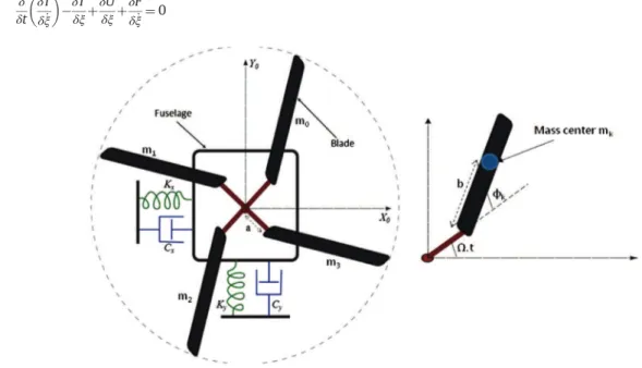
In this section, the suggested identification method is tested on a helicopter model. We give, first, some essential elements that allow to understand the dynamics of a helicopter on the ground and the instabilities that may occur, namely the ground resonance.
When the rotor of a helicopter is spinning, some angular phase shifts – known as leading and lagging angles – can be created on the blades by external disturbances. Basically, this may occur when a helicopter with a wheel-type landing gear touches the ground firmly on one corner, then this shock is transmitted to the blades in the form of out of phase angular motions. Those angular motions interact with the elastic parts of the fuselage (the landing gear, mainly) for certain values of rotor's angular velocity. The fuselage starts then to rock laterally. These lateral oscillations amplify the lead-lagging motions which also amplify the fuselage oscillations, and so on till the divergence and the destruction of the structure when a critical rotation velocity is reached.
The analysis given herein is based on the model in[41], but extending it to the case where dampers are present on the structure. The fuselage is considered to be a rigid body with mass M, attached to a flexible landing gear (LG) which is modeled by two springs Kxand Ky, and two viscous dampers Cxand Cyas illustrated inFig. 2. For the sake of simplicity, the fuselage is
considered to be symmetrical: namely the stiffnesses are equal to the same value, Kz, Kx¼ Ky¼ Kzand idem for the viscous
dampers Cx¼ Cy¼ Cz. The rotor spinning with a velocity Ω is articulated and the offset between the MR (main rotor) and each
articulation is noted as a. For k ¼ 0; …; Nb'1 (with Nbthe number of blades), each blade is modeled by a concentrated mass m –
considered constant here for the sake of simplicity – at a distance b of the articulation point and a torque stiffness and a viscous damping Kϕkand Cϕkare present in each articulation. The moment of inertia around each articulation point is Iz. The degrees of freedom are the lateral displacements of the fuselage x and y, and the out-of-phase angles ðϕkÞ.
The equation of motion of the studied mechanical system is obtained by applying Lagrange equations to the kinetic, potential energy and dissipation function's expressions (respectively T, U and F) of the helicopter, given inAppendix B:
δ δt δT δ_ξ 5 6 'δT δξþ δU δξþ δF δ _ξ¼ 0 ð35Þ
ξ is a dummy variable which is replaced by the system variables. Let q be the vector containing these variables q ¼ ½x; y; ϕ0; ϕ1; …; ϕNb'1+
T. In our case, the behavior of the helicopter is described by the equation:
MðtÞ €q þCðtÞ _q þKðtÞq ¼ 0 ð36Þ
The matrices M, C and K are respectively mass, stiffness and damping matrices. Their expressions are given inAppendix C. The system matrices are periodic with a period T ¼ 2π=Ω:
Mðt þTÞ ¼ MðtÞ; Cðt þTÞ ¼ CðtÞ; Kðt þTÞ ¼ KðtÞ; 8t Z0 ð37Þ The model can be rewritten as in(18), taking the state variable XðtÞ ¼ ½qðtÞ
_
qðtÞ+ and the state matrix AðtÞ ¼ ½'M'10ðtÞKðtÞ'M'1IðtÞCðtÞ+ where I is the identity matrix.
4.2. Numerical simulation
Let us consider a helicopter with 4-bladed rotor, for this numerical application. And let the numerical values inTable 1be the structural parameters of the considered helicopter. The numerical values are those of the model in[41], adding viscous dampers to it. In order to mimic the dynamics of a real helicopter, the values of the damping coefficients are taken such that Cx¼ Kx=25 and Cϕ¼ Kϕ=25 as in[42].
A standard white Gaussian signal with a unit standard deviation svis generated for the state noise v. A white Gaussian
noise w with a standard deviation sw is also generated such that the ratio sv=sw¼ 103. To simulate an anisotropy in the
rotor, the stiffness of the fourth blade is taken such that Kϕ3¼ 0:75Kϕ. We take the observation matrix C ¼ ½010%2I10%10+.
To simulate the data yk, Eq.(14)is numerically integrated using the Runge–Kutta method.
4.3. Identification results
For Ω ¼ 3:5 rad=s, a first data set is generated over a number of rotor revolutions NT¼2000, with a discrete period
Td¼100 (the sampling frequency is Fs¼ Td=T). The order of the system is assumed to be known and is n ¼12. The suggested
identification algorithm is applied to the data as explained herein before. The parameters p and q are chosen such that q ¼ pþ1 ¼ 31. The summary of the identified frequencies and damping ratios using the classical and the new SSI algorithms, as well as the true values, is given inTable 2. For each value of Ω, the new SSI is performed using NT¼2000 data samples
where the classical algorithm uses N¼200,000 samples. For the true modes, the monodromy matrix is computed from the Runge–Kutta numerical integration Q ¼ eR0TAðtÞ dt. Then, the eigenvalues and the corresponding modal parameters (frequency and damping ratio) are deduced using(20).
Table 1
Structural properties for hinged-blades helicopter with 4 blades[41]. Structural variable Name Value
Blade mass m 31.9 kg Fuselage mass M 2902.9 kg Blade stiffness Kϕ 1.0313 % 103N/m
LG stiffness in the axis x Kx 2.7275 % 104N/m
LG stiffness in the axis y Ky 2.7275 % 104N/m
Blade damping coef. Cϕ 41.252 N s/m
LG damping in the axis x Cx 1.091 % 103N s/m
LG damping in the axis y Cy 1.091 % 103N s/m
Rotor eccentricity a 0.2 m Blade length b 2.5 m Blade inertial moment Iz 259 kg m2
Table 2
Classical and new algorithms results compared to true values for Ω ¼ 3:5 rad=s.
Mode Classical SSI New SSI True values
Freq. (Hz) D. ratio Freq. (Hz) D. ratio Freq. (Hz) D. ratio 1 0.4769 0.1124 0.0853 0.3393 0.0850 0.3384 2 0.485 0.0526 0.0939 0.2948 0.0928 0.2936 3 0.2263 0.0438 0.2277 0.0396 0.234 0.0316 4 0.2567 0.022 0.2589 0.0306 0.2597 0.0276 5 0.259 0.033 0.2607 0.0274 0.2604 0.0275 6 0.273 0.05 0.2744 0.0385 0.2751 0.0324
The classical SSI algorithm identifies some modes but is largely wrong for the first two modes. The new algorithm identifies all the modes and is more accurate for the last four modes thought it uses much less data samples than the classical algorithm. This identification goes of course more accurate when the sample length gets larger as shown inTable 3where the relative errors of the identified frequencies using the new algorithms are computed for NT¼2000 and NT¼ 10; 000.
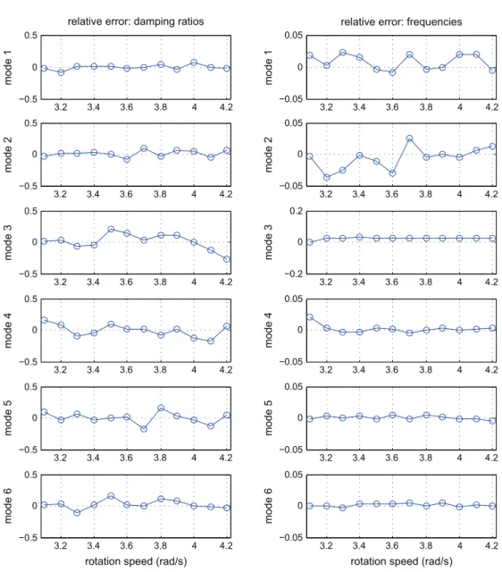
The new algorithm is also applied for simulation data set with varying rotation speed Ω from 3.1 rad/s to 4.2 rad/s by a step of 0.1 rad/s, and data were simulated over a number NT¼2000 of periods for each step of Ω. The relative errors of the
new algorithm are plotted toward the rotation speed and reported inFig. 3. The variation of the identified frequencies and
Table 3
Variation of relative errors for new SSI with respect to sample length. Mode Frequency error
(NT¼2000) Frequency error (NT¼ 10; 000) 1 0.0232 0.0082 3 0.0370 '0.0032 3 0.0288 0.0013 4 0.0209 '0.0012 5 0.0045 '0.0004 6 0.0050 '0.0007 3.2 3.4 3.6 3.8 4 4.2 −0.05 0 0.05 mode 1
relative error: frequencies
3.2 3.4 3.6 3.8 4 4.2 −0.05 0 0.05 mode 2 3.2 3.4 3.6 3.8 4 4.2 −0.2 0 0.2 mode 3 3.2 3.4 3.6 3.8 4 4.2 −0.05 0 0.05 mode 4 3.2 3.4 3.6 3.8 4 4.2 −0.05 0 0.05 mode 5 3.2 3.4 3.6 3.8 4 4.2 −0.05 0 0.05 mode 6
rotation speed (rad/s)
3.2 3.4 3.6 3.8 4 4.2
−0.5 0 0.5
mode 1
relative error: damping ratios
3.2 3.4 3.6 3.8 4 4.2 −0.5 0 0.5 mode 2 3.2 3.4 3.6 3.8 4 4.2 −0.5 0 0.5 mode 3 3.2 3.4 3.6 3.8 4 4.2 −0.5 0 0.5 mode 4 3.2 3.4 3.6 3.8 4 4.2 −0.5 0 0.5 mode 5 3.2 3.4 3.6 3.8 4 4.2 −0.5 0 0.5 mode 6
rotation speed (rad/s)
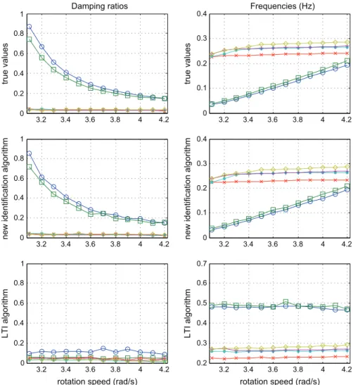
damping ratios using the new and the classical algorithms, as well as the variation of the true values, is given inFig. 4. One can notice that the modes identified by the new algorithm track the true modes, whereas the classical algorithm gives modes with different variations.
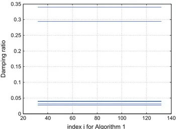
Another feature to test is that these identified frequencies and damping ratios do not change over time as shown in Eq.(21), for a different choice of the index j (j being a parameter forAlgorithm 1) (seeFig. 1). The variation of the estimated frequencies and damping ratios is plotted at Ω ¼ 3:5 rad=s, over a period (from the sample j¼q to j ¼ qþTd), and they are
indeed constant as shown inFigs. 5and6.
It is also important to notice that the classical algorithm manages to identify correctly some of the modes (Table 2), because the considered rotation speed is close to the critical speed Ω ¼ 4:4 rad=s of the ground resonance where the fuselage (time-invariant part) and the rotor (time-periodic part) are coupled. When the rotation speed is far from 4.4 rad/s, this classical algorithm gives totally irrelevant results.Table 4shows this for Ω ¼ 2 rad=s, for example. It shows the identified frequencies using the two algorithms as well as the true frequencies. The classical algorithm uses much more data samples N¼200,000 than the new algorithm NT¼2000, however its identified modes are still highly biased.
4.4. Comparison with other approaches
As mentioned in the Introduction, works on the identification of LPTV systems remain limited. Under the assumption of isotropy, the identification could be handled with the so-called Coleman transformation or multi-blade transformation (MBC)[43], which allows to write the underlying system in the rotating frame, and then to obtain a time-invariant model. This approach has been recently suggested in[44]where the MBC transform is used as a pre-processing step to the classical SSI algorithm. The isotropy assumption must be not only internal but external, also: the rotor blades of the considered system have the same static structural properties, and the external loads are symmetric [37]. The latter symmetry is
3.2 3.4 3.6 3.8 4 4.2 0 0.1 0.2 0.3 0.4 true values Frequencies (Hz) 3.2 3.4 3.6 3.8 4 4.2 0 0.1 0.2 0.3 0.4
new identification algorithm
3.2 3.4 3.6 3.8 4 4.2 0.2 0.3 0.4 0.5 0.6 0.7
rotation speed (rad/s)
LTI algorithm 3.2 3.4 3.6 3.8 4 4.2 0 0.2 0.4 0.6 0.8 1 true values Damping ratios 3.2 3.4 3.6 3.8 4 4.2 0 0.2 0.4 0.6 0.8 1
new identification algorithm
3.2 3.4 3.6 3.8 4 4.2 0 0.2 0.4 0.6 0.8 1
rotation speed (rad/s)
LTI algorithm
Fig. 4. Modes variation w.r.t. rotation speed Ω. On the left: the damping ratios. On the right: the frequencies. The top two figures are the true values. The bottom two figures: identification results by the classical SSI algorithm. And in the middle: identification results by the new SSI.
guaranteed when the system is operating in vacuum and is then quickly violated for real applications. In fact, the dynamic properties of the system (mainly the dynamic stiffnesses) may change drastically with the external loads such as aero-elastic and gravity loads as shown in[45,37]. In this case, the inherent periodic behavior cannot be completely suppressed and should be taken into account for the modal analysis[45,46]. This analysis is provided by the Floquet theory.
To the authors' knowledge, the work of Allen in[26]is the only work which deals with the output-only identification of the Floquet modes. The suggested approach uses a theory developed by Wereley in [29] regarding harmonic transfer functions (HTF), and the expression of the output spectrum in terms of the Floquet modes in order to estimate these latter
20 40 60 80 100 120 140 0 0.05 0.1 0.15 0.2 0.25 0.3 0.35
index j for Algorithm 1
Damping ratio
Fig. 5. Damping estimates for index j, over a period, forAlgorithm 1at Ω ¼ 3:5 rad=s.
20 40 60 80 100 120 140 0.08 0.1 0.12 0.14 0.16 0.18 0.2 0.22 0.24 0.26 0.28
index j for Algorithm 1
Frequency (Hz)
Fig. 6. Frequency estimates for index j, over a period, forAlgorithm 1at Ω ¼ 3:5 rad=s.
Table 4
Frequency estimates compared to true values for Ω ¼ 2 rad=s. Mode Classical SSI (Hz) New SSI (Hz) True values (Hz) 1 0.2171 0.0576 0.0586 2 0.2451 0.0732 0.0728 3 0.2451 0.0732 0.0728 4 0.2527 0.0995 0.0997 5 0.4791 0.1458 0.1481 6 0.4807 0.1559 0.1617
modes with the peak picking technique. As mentioned by Allen, the picking is based on a prior knowledge about the system and some spectra rays were neglected and were still uninterpreted.
The approach presented in the current paper does not require a prior knowledge of system dynamics and seems to give good estimates of the Floquet modes. At first sight, having fewer points for the new SSI algorithm (NT¼ N=Td) may appear as
a potential drawback compared to the classical SSI which uses more data samples. This drawback is overcome by the fact that the new algorithm is not biased unlike the classical one as illustrated by the numerical application.
Besides, an algorithm is defined by its bias (consistency) and variance properties (efficiency). In this paper, it has been demonstrated that for one realization of the noise sequence, the algorithm provides estimated quantities close to the true ones. Considerations on the efficiency are pure assumptions and conjectures at this point. It has to be proved by a much heavier tool set. Efficiency of subspace methods for linear time-invariant approaches has been considered by the authors recently (see[47]). The extension of this study to the algorithm suggested herein is the scope of a future work.
5. Conclusion
The problem of identification for linear periodically time-varying is addressed. A new subspace-based algorithm is proposed. It has the aim to identify the so-called discrete-time monodromy matrix and its eigenvalues. This matrix is derived from the Floquet transformation which gives an equivalent description of periodic systems. Its eigenvalues, the Floquet multipliers, replace the classical eigenvalues in the classical modal analysis for linear time-invariant systems.
For this, a subspace matrix was built over lagged output data subsequences. Then, the matrix was extracted from a least squares minimization equation. The suggested algorithm is finally tested on data created from the simulation of a hinged blades helicopter spinning on the ground. Future works will focus on both the estimation of the uncertainties associated to the identified parameters and the validation with experimental data from helicopters and wind turbines.
Appendix A. Proof of Proposition 3.1
The elements of the Hankel matrix in(24)are products between lagged outputs yj þ mand yj'l. These products write yj þ myT j'l¼C~j þ mFm þ lzj'lyTj'l þC~j þ mFm þ l'1v~ j'l þ 1yTj'l þC~j þ mFm þ l'2v~ j'l þ 2yTj'l þ⋯ þC~j þ mF ~vj þ m'1yT j'l þC~j þ mv~ j þ myTj'l þwj þ myTj'l ðA:1Þ
The observation matrix ~C is periodic. Then ~Cj þ iTd¼ ~
Cj, 8i40. Now, let us compute the sum:
∑ NT'1 i ¼ 0 yj þ m þ iTdyT j'l þ iTd¼ ~ Cj þ mFm þ lN∑T'1 i ¼ 0 zj'l þ iTdyT j'l þ iTd þC~j þ mFm þ l'1 ∑ NT'1 i ¼ 0 ~ vj'l þ 1 þ iTdyT j'l þ iTd þ⋯ þC~j þ mF ∑NT'1 i ¼ 0 ~ vj þ m'1 þ iTdyT j'l þ iTd þC~j þ mN∑T'1 i ¼ 0 ~ vj þ m þ iTdyT j'l þ iTd þ ∑ NT'1 i ¼ 0 wj þ m þ iTdyT j'l þ iTd ðA:2Þ
Dividing by NTleads to:
/
C~j þ mFm þ lð1=NTÞ∑Ni ¼ 0T'1zj'l þ iTdy
T
j'l þ iTd converges to ~Cj þ mF
m þ lGðj'lÞ when N
T goes large, where Gðj'lÞ is the correlation
between the ðj'lÞ'th time-invariant subsequences of the state vector and the output vector.
/
C~j þ mFm þ l'1ð1=NTÞ∑Ni ¼ 0T'1v~j'l þ 1 þ iTdy
T
j'l þ iTd converges to 0 when NT goes large, because w is a white noise which is uncorrelated of any time-invariant subsequence of the output, idem for ~Cj þ mFm þ l'2ð1=NTÞ∑Ni ¼ 0T'1v~j'l þ 2 þ iTdy
T j'l þ iTd, …, ~ Cj þ mFð1=NTÞ∑Ni ¼ 0T'1v~j þ m'1 þ iTdy T j'l þ iTd and ~Cj þ mð1=NTÞ∑ NT'1 i ¼ 0v~j þ m þ iTdy T j'l þ iTd.
/
ð1=NTÞ∑Ni ¼ 0T'1wj þ m þ iTdy Tj'l þ iTd converges to 0 too (unless when m ¼ l ¼ 0, which is not the case herein), for the same reason of uncorrelation.
Appendix B. Energies' expressions B.1. Kinetic energy
According to the theorem of Koenig, the total kinetic energy of one blade is the sum of the kinetic energy of the circular translation, and that of the rotation about the center of mass of the blade:
Tpk¼12m_zkz_kþ12Izϕ_2k ðB:1Þ
where m is the mass of the blade, Ω is the angular velocity of the main rotor, Izis the moment of inertia of the k-th blade
about its center of mass, z ¼ xþiy and zk¼ xkþiyk¼ zþðaþbeiϕkÞeiðΩt þ αkÞ is the coordinate of the k-th blade, with
α¼ 2π=ðNb'1Þ and Nbis the number of blades. Then for small displacements ϕk, the kinetic energy of one blade writes
Tpk¼12m½_zz þ_ z ibð_ ϕ_kþiΩϕkÞeiðΩt þ αkÞþ _zð'ibÞðϕ_k'iΩϕkÞe'iðΩt þ αkÞ
þb2ϕ_2k'Ω2abϕk2+þ12Izϕ_2k ðB:2Þ
Finally, the total kinetic energy of the helicopter writes T ¼12M _zz þ ∑_ Nb'1
k ¼ 0
Tpk ðB:3Þ
B.2. Potential energy
The potential energy of the helicopter originates from the stiffnesses of the fuselage in the two directions x and y, modeled inFig. 2by two springs, and the stiffnesses of the Nbblades. The total potential energy is then the sum of the
separate energies: U ¼12Kzzz þ 1 2 ∑ Nb'1 k ¼ 0 Kϕkϕ 2 k ðB:4Þ B.3. Dissipation function
Dampers are added to the model considered in[41]. Its incorporation in the structure provides more stability to it, by absorbing the oscillation of the landing gear and reducing the lead lagging modes on the rotor. This stabilizing effect is discussed in[48,49] who considered dampers on the rotor. The dampers are assumed to be linear. Nonlinear dampers can be replaced by equivalent linear viscous damping using a standard linearization technique[50]. Similar to the potential energy, the dissipation function can be written as
F ¼12Czz_z þ_ 12 ∑ Nb'1 k ¼ 0 Cϕk _ ϕ2k ðB:5Þ
Appendix C. System matrices The system matrices write
M¼
ðM þNbmÞ 0 'mb: sin0 ⋯ ⋯ 'mb:ð sin ÞNb'1 0 ðM þNbmÞ mb: cos0 ⋯ ⋯ mb:ð cos ÞNb'1 'mb: sin0 mb: cos0 ðmb2þIzÞ 0 ⋯ 0
⋮ ⋮ ⋮ ⋱ 'mb:ð sin ÞNb'1 mb:ð cos ÞNb'1 0 0 ⋯ ðmb 2 þIzÞ 2 6 6 6 6 6 6 6 4 3 7 7 7 7 7 7 7 5 C¼ Cx 0 '2 mbΩ: cos0 ⋯ '2 mbΩ:ð cos ÞNb'1 Cy '2 mbΩ: sin0 ⋯ '2 mbΩ:ð sin ÞNb'1 Cϕ0 ⋱ CϕNb'1 2 6 6 6 6 6 6 6 4 3 7 7 7 7 7 7 7 5
K¼ Kx 0 mbΩ2: sin0 ⋯ mbΩ2:ð sin ÞNb'1 Ky 'mbΩ2: cos0 ⋯ 'mbΩ2:ð cos ÞNb'1 Kϕ0þmΩ 2ab ⋱ KϕNb'1þmΩ2ab 2 6 6 6 6 6 6 6 4 3 7 7 7 7 7 7 7 5
where sink¼ sin ðΩt þαkÞ, cosk¼ cos ðΩt þαkÞ and α ¼ 2π=ðNb'1Þ.
References
[1]C. Desoer, Slowly varying discrete system xiþ1 ¼ aixi, Electronics Letters 6 (11) (1970) 339–340.
[2]M. Freedman, G. Zames, Logarithmic variation criteria for the stability of systems with time-varying gains, SIAM Journal on Control 6 (3) (1968) 487–507.
[3]L. Ljung, System Identification: Theory for the User, vol. 7632, Prentice Hall, New Jersey, 1987. [4]A.H. Sayed, Fundamentals of Adaptive Filtering, John Wiley & Sons, 2003.
[5]Y. Li, H.-l. Wei, S.A. Billings, Identification of time-varying systems using multi-wavelet basis functions, IEEE Transactions on Control Systems Technology 19 (3) (2011) 656–663.
[6]R. Zou, H. Wang, K.H. Chon, A robust time-varying identification algorithm using basis functions, Annals of Biomedical Engineering 31 (7) (2003) 840–853.
[7]Z. Qizhi, L. Li, Identification of time-varying system based on fourier series, in: WRI Global Congress on Intelligent Systems, GCIS'09, vol. 2, IEEE, 2009, pp. 44–47.
[8]M. Niedzwiecki, T. Klaput, Fast recursive basis function estimators for identification of time-varying processes, IEEE Transactions on Signal Processing 50 (8) (2002) 1925–1934.
[9]M. Verhaegen, X. Yu, A class of subspace model identification algorithms to identify periodically and arbitrarily time-varying systems, Automatica 31 (2) (1995) 201–216.
[10]K. Liu, Identification of linear time-varying systems, Journal of Sound and Vibration 206 (4) (1997) 487–505.
[11] K. Liu, Extension of modal analysis to linear time-varying systems, Journal of Sound and Vibration 226 (1) (1999) 149–167.
[12]K. Liu, L. Deng, Experimental verification of an algorithm for identification of linear time-varying systems, Journal of Sound and Vibration 279 (3) (2005) 1170–1180.
[13]P. Van Overschee, B. De Moor, Subspace Identification for Linear Systems: Theory, Implementation, Applications, Kluwer Academic Publishers, 1996. [14]M. Majji, J.-N. Juang, J.L. Junkins, Time-varying eigensystem realization algorithm, Journal of Guidance, Control, and Dynamics 33 (1) (2010) 13–28. [15]K. Josic, R. Rosenbaum, Unstable solutions of nonautonomous linear differential equations, SIAM Review 50 (3) (2008) 570–584.
[16]É. Mathieu, Mémoire sur le mouvement vibratoire d’une membrane de forme elliptique, Journal de mathématiques pures et appliquées 2e série, tome 13 (1868) 137–203.
[17]G. Floquet, Sur les équations différentielles linéaires à coefficients périodiques, Annales Scientifiques de l’École Normale Supérieure 12 (1883) 47–88. [18]J.A. Richards, Analysis of Periodically Time-varying Systems, Springer-Verlag, Berlin, 1983.
[19]P. Montagnier, C.C. Paige, R.J. Spiteri, Real Floquet factors of linear time-periodic systems, Systems & Control Letters 50 (4) (2003) 251–262. [20] S. Bittanti, P. Colaneri, Periodic Systems: Filtering and Control, Springer, London, 2009.
[21]L. Sanches, G. Michon, A. Berlioz, D. Alazard, Instability zones for isotropic and anisotropic multibladed rotor configurations, Mechanism and Machine Theory 46 (8) (2011) 1054–1065.
[22] L. Sanches, G. Michon, A. Berlioz, D. Alazard, Parametrically excited helicopter ground resonance dynamics with high blade asymmetries, Journal of Sound and Vibration 331 (16) (2012) 3897–3913.
[23] C.C. Ross, Differential Equations: An Introduction with Mathematicas, Springer, 2004.
[24] S.C. Sinha, E. Butcher, Symbolic computation of fundamental solution matrices for linear time-periodic dynamical systems, Journal of Sound and Vibration 206 (1) (1997) 61–85.
[25] E.A. Butcher, H. Ma, E. Bueler, V. Averina, Z. Szabo, Stability of linear time-periodic delay-differential equations via Chebyshev polynomials, International Journal for Numerical Methods in Engineering 59 (7) (2004) 895–922.
[26] M.S. Allen, M.W. Sracic, S. Chauhan, M.H. Hansen, Output-only modal analysis of linear time-periodic systems with application to wind turbine simulation data, Mechanical Systems and Signal Processing 25 (4) (2011) 1174–1191.
[27]M. Allen, J.H. Ginsberg, Floquet modal analysis to detect cracks in a rotating shaft on anisotropic supports, in: 24th International Modal Analysis Conference (IMAC XXIV), 2006.
[28] M. Allen, Floquet experimental modal analysis for system identification of linear time-periodic systems, in: ASME 2007 International Design Engineering Technical Conferences & Computers and Information in Engineering Conference, 2007.
[29] N.M. Wereley, S.R. Hall, Frequency response of linear time periodic systems, in: Proceedings of the 29th IEEE Conference on Decision and Control, IEEE, 1990, pp. 3650–3655.
[30] A. Benveniste, J.-J. Fuchs, Single sample modal identification of a nonstationary stochastic process, IEEE Transactions on Automatic Control 30 (1) (1985) 66–74.
[31]T. Soderstrom, P. Stoica, System Identification, Prentice Hall International Series in Systems and Control Engineering, 1989.
[32] B. Peeters, G. De Roeck, Reference-based stochastic subspace identification for output-only modal analysis, Mechanical Systems and Signal Processing 13 (6) (1999) 855–878.
[33] M. Basseville, A. Benveniste, M. Goursat, L. Hermans, L. Mevel, et al., Output-only subspace-based structural identification: from theory to industrial testing practice, ASME Journal of Dynamic Systems, Measurement, and Control 123 (4) (2001) 668–676. (Special issue on Identification of mechanical systems).
[34] M. Goursat, L. Mevel, Algorithms for covariance subspace identification: a choice of effective implementations, in: Proceedings of the IMAC XXVII, Florida, USA, 2009.
[35] M. Basseville, M. Abdelghani, A. Benveniste, Subspace-based fault detection algorithms for vibration monitoring, Automatica 36 (1) (2000) 101–109. [36] J.J. DaCunha, J.M. Davis, A unified Floquet theory for discrete, continuous, and hybrid periodic linear systems, Journal of Differential Equations 251 (11)
(2011) 2987–3027.
[37]P. Skjoldan, Aeroelastic Modal Dynamics of Wind Turbines Including Anisotropic Effects, Ph.D. Thesis, Technical University of Denmark, 2011.
[38] R. Meyer, C. Burrus, A unified analysis of multirate and periodically time-varying digital filters, IEEE Transactions on Circuits and Systems 22 (3) (1975) 162–168.
[39] A. Jhinaoui, L. Mevel, J. Morlier, Subspace identification for linear periodically time-varying systems, in: Proceedings of the 16th IFAC Symposium on System Identification (SYSID), 2012, pp. 1282–1287.
[40] A. Jhinaoui, L. Mevel, J. Morlier, Extension of subspace identification to lptv systems: application to helicopters, in: Topics in Modal Analysis I, vol. 5, Springer, 2012, pp. 425–433.
[41]L. Sanches, G. Michon, A. Berlioz, D. Alazard, Instability zones identification in multiblade rotor dynamics, in: 11th Pan-American Congress of Applied Mechanics, 2010.
[42] J. Wang, I. Chopra, Dynamics of helicopters in ground resonance with and without blade dissimilarities, in: AIAA Dynamics Specialists Conference, Dallas, TX, 1992, pp. 273–291.
[43] G. Bir, Multi-blade coordinate transformation and its applications to wind turbine analysis, in: ASME Wind Energy Symposium, 2008.
[44]D. Tcherniak, S. Chauhan, M. Rossetti, I. Font, J. Basurko, O. Salgado, Output-only modal analysis on operating wind turbines: application to simulated data, in: European Wind Energy Conference, 2010.
[45] K. Stol, H. Moll, G. Bir, H. Namik, A comparison of multi-blade coordinate transformation and direct periodic techniques for wind turbine control design, in: 47th AIAA Aerospace Sciences Meeting, 2009.
[46] L. Sanches, Helicopter Ground Resonance: Dynamical Modeling, Parametric Robustness Analysis and Experimental Validation, Ph.D. Thesis, ISAE, 2011.
[47]M. Döhler, X.-B. Lam, L. Mevel, Uncertainty quantification for modal parameters from stochastic subspace identification on multi-setup measurements, Mechanical Systems and Signal Processing 36 (2013) 562–581.
[48]D.L. Kunz, Influence of elastomeric damper modeling on the dynamic response of helicopter rotors, AIAA Journal 35 (1997) 349–354. [49]D.L. Kunz, Nonlinear analysis of helicopter ground resonance, Nonlinear Analysis: Real World Applications 3 (3) (2002) 383–395.
[50] L. Pang, G.M. Kamath, N.M. Wereley, Analysis and testing of a linear stroke magnetorheological damper, in: Proceedings of the 39th AIAA/ASME/ASCE/ AHS/ASC Structures, Structural Dynamics, and Materials Conference and Exhibit and AIAA/ASME/AHS Adaptive Structures Forum, 1998, pp. 2841– 2856.