O
pen
A
rchive
T
OULOUSE
A
rchive
O
uverte (
OATAO
)
OATAO is an open access repository that collects the work of Toulouse researchers and
makes it freely available over the web where possible.
This is an author-deposited version published in :
http://oatao.univ-toulouse.fr/
Eprints ID : 15495
The contribution was presented at :
http://liris.cnrs.fr/ismis15/
Official URL: http://dx.doi.org/10.1007/978-3-319-25252-0_21
To cite this version : The Cube of Opposition and the Complete Appraisal of
Situations by Means of Sugeno Integrals. (2015) In: 22nd International Symposium
on Methodologies for Intelligent Systems (ISMIS 2015), 21 October 2015 - 23
October 2015 (Lyon, France).
Any correspondance concerning this service should be sent to the repository
administrator: [email protected]
The cube of opposition and the complete appraisal of
situations by means of Sugeno integrals
Didier Dubois1, Henri Prade1, and Agn`es Rico2(B)
1
IRIT, Universit´e Paul Sabatier
118 route de Narbonne, 31062 Toulouse cedex 9 (France)
2
ERIC, Universit´e Claude Bernard Lyon 1 43 bld du 11 novembre 69100 Villeurbanne (France)
Abstract. The cube of opposition is a logical structure that underlies many in-formation representation settings. When applied to multiple criteria decision, it displays various possible aggregation attitudes. Situations are usually assessed by combinations of properties they satisfy, but also by combinations of proper-ties they do not satisfy. The cube of opposition applies to qualitative evaluation when criteria are weighted as well as in the general case where any subset of criteria may be weighted for expressing synergies between them, as for Sugeno integrals. Sugeno integrals are well-known as a powerful qualitative aggregation tool which takes into account positive synergies between properties. When there are negative synergies between properties we can use the so-called desintegral associated to the Sugeno integral. The paper investigates the use of the cube of opposition and of the if-then rules extracted from these integrals and desintegrals in order to better describe acceptable situations.
1
Introduction
The description of situations (or objects, or items) is usually based on the degrees to which they satisfy properties (or criteria). Sugeno integrals [12, 13] are qualitative in-tegrals first used as aggregation operators in multiple criteria decision. They deliver a global evaluation between the minimum and the maximum of the partial evaluations. The definition of the Sugeno integral is based on a monotonic set function, called ca-pacity or fuzzy measure, which represents the importance of the subsets of criteria.
More recently Sugeno integrals have been used as a representation tool for describ-ing more or less acceptable objects [11] under a bipolar view. In such a context the prop-erties are supposed to be positive, i.e, the global evaluation increases with the partial ratings. But some objects can be accepted because they don’t satisfy some properties. So we also need to consider negative properties, i.e., the global evaluation increases when the partial ratings decreases. Hence a pair of evaluations made of a Sugeno inte-gral and a reversed Sugeno inteinte-gral are used to describe acceptable objects in terms of properties they must have and of properties they must avoid. This reversed integral is a variant of Sugeno integral, called a desintegral. Their definition is based on a decreasing set function called anti-capacity.
Moreover, it was proved that the Sugeno integrals and the associated desintegrals can be encoded as a possibilistic logic base [7, 5]. These results have been used for
extracting decision rules from qualitative data evaluated on the basis of Sugeno integrals [1]. This paper extends these results to the extraction of decision rules from qualitative data using qualitative desintegrals. These decision rules should help completing the results presented in [11].
Besides, we can distinguish the optimistic part and the pessimistic part of any pacity [8]. It has been recently indicated that Sugeno integrals associated to these ca-pacities and their associated desintegrals form a cube of opposition [9], the integrals being present on the front facet and the desintegrals on the back facet of the cube (each of these two facets fit with the traditional views of squares of opposition). As this cube summarizes all the evaluation options, we may consider the different Sugeno integrals and desintegrals present on the cube in the selection process of acceptable situations.
The paper is organized as follows. Section 2 introduces the cube of opposition and discusses its relevance for multiple criteria aggregation. Section 3 restates the main results on Sugeno integrals, desintegrals, and their logical rule counterparts, before pre-senting the cube of opposition for Sugeno integrals and desintegrals in section 4. Section 5 takes advantage of the cube for discussing the different aggregation attitudes and their relations.
2
Square and cube of opposition in multiple criteria evaluation
The traditional square of opposition [10] is built with universally and existentially quan-tified statements in the following way. Consider a statement (A) of the form “all P ’s are Q’s”, which is negated by the statement (O) “at least one P is not a Q”, together with the statement (E) “no P is a Q”, which is clearly in even stronger opposition to the first statement (A). These three statements, together with the negation of the last statement, namely (I) “at least one P is a Q” can be displayed on a square whose vertices are traditionally denoted by the letters A, I (affirmative half) and E, O (negative half), as pictured in Figure 1 (where Q stands for “not Q”).
Contraries
A: all P ’s are Q’s E: all P ’s are Q’s
Sub-alterns
Sub-contraries
I: at least one P is a Q O: at least one P is a Q
Sub-alterns Contrad ict ories Contr a dictorie s
Fig. 1. Square of opposition As can be checked, noticeable relations hold in the square: - (i) A and O (resp. E and I) are the negation of each other;
- (ii) A entails I, and E entails O (it is assumed that there is at least one P for avoiding existential import problems);
- (iii) together A and E cannot be true, but may be false ; - (iv) together I and O cannot be false, but may be true.
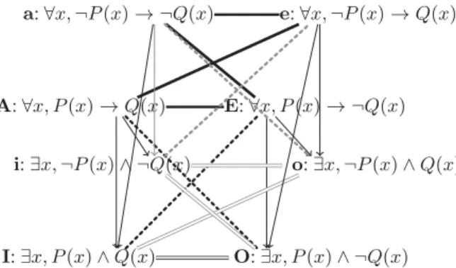
Changing P into¬P , and Q in ¬Q leads to another similar square of opposition aeoi, where we also assume that the set of “not-P ’s” is non-empty. Then the 8 state-ments, A, I, E, O, a, i, e, o may be organized in what may be called a cube of opposition [4] as in Figure 2. i: ∃x, ¬P(x) ∧ ¬Q(x) I: ∃x, P(x) ∧ Q(x) O: ∃x, P(x) ∧ ¬Q(x) o: ∃x, ¬P(x) ∧ Q(x) a: ∀x, ¬P(x) → ¬Q(x) A: ∀x, P(x) → Q(x) E: ∀x, P(x) → ¬Q(x) e: ∀x, ¬P(x) → Q(x)
Fig. 2. Cube of opposition of quantified statements
The front facet and the back facet of the cube are traditional squares of opposition. In the cube, if we also assume that the sets of “Q’s” and “not-Q’s” are non-empty, then the thick non-directed segments relate contraries, the double thin non-directed segments sub-contraries, the diagonal dotted non-directed lines contradictories, and the vertical uni-directed segments point to subalterns, and express entailments. Stated in set vocab-ulary, A, I, E, O, a, i, e, o, respectively means P ⊆ Q, P ∩ Q 6= ∅, P ⊆ Q, P ∩ Q 6= ∅, P ⊆ Q, P ∩ Q 6= ∅, P ⊆ Q, P ∩ Q 6= ∅. In order to satisfy the four conditions of a square of opposition for the front and the back facets, we need P 6= ∅ and P 6= ∅. In order to have the inclusions indicated by the diagonal arrows in the side facets, we need Q6= ∅ and Q 6= ∅ as further normalization conditions.
Suppose P denotes a set of important properties, Q a set of satisfied properties (for a considered object). Vertices A, I, a, i correspond respectively to 4 different cases: i) all important properties are satisfied, ii) at least one important property is satisfied, iii) all satisfied properties are important, iv) at least one non satisfied property is not important. Note also the cube is compatible with an understanding having a bipolar flavor [3]. Suppose that among possible properties for the considered objects, some are desirable (or requested) and form a subset R and some others are excluded (or undesirable) and form a subset E. Clearly, one should have E ⊆ R. For a considered object the set of properties is partitioned into the subset of satisfied properties S and the subset S of properties not satisfied. Then vertex A corresponds to R⊆ S and a to R ⊆ S. Then a also corresponds to E⊆ S.
More generally, satisfaction of properties may be graded, and importance (both with respect to desirability and undesiraribility) is also a matter of degree. It is the case in multiple criteria aggregation where objects are evaluated by means of a setC of criteria i (where1 ≤ i ≤ n). Let us denote by xithe evaluation of a given object for criterion
i, and x = (x1,· · · , xi,· · · , xn). We assume here that ∀i, xi ∈ [0, 1]. xi = 1 means
satisfaction. Let πi ∈ [0, 1] represent the level of importance of criterion i. The larger
πithe more important the criterion.
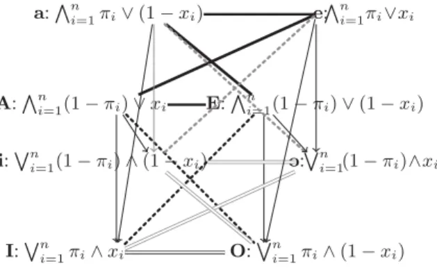
Simple qualitative aggregation operators are the weighted min and the weighted max [2]. The first one measures the extent to which all important criteria are satisfied; it corresponds to the expressionVni=1(1 − πi) ∨ xi, while the second one,Wni=1πi∧ xi,
is optimistic and only requires that at least one important criterion be highly satisfied. Under the hypothesis of the double normalization (∃i, πi= 1 and ∃j, πj = 0) and the
hypothesis∃r, xr= 1 and ∃s, xs= 0 , weighted min and weighted max correspond to
vertices A and I of the cube on Fig. 3.
i:Wni=1(1 − πi) ∧ (1 − xi) I:Wni=1πi∧xi O: Wn i=1πi∧(1 − xi) o:Wni=1(1 − πi)∧xi a:Vni=1πi∨(1 − xi) A:Vni=1(1 − πi) ∨ xi E: Vn i=1(1 − πi) ∨ (1 − xi) e:Vni=1πi∨xi
Fig. 3. Cube of weighted qualitative aggregations
There is a correspondance between the aggregation functions on the right facet and those on the left facet, replacing x with1 − x.
Suppose that a fully satisfied object x is an object with an global rating equal to1. Vertices A, I, a and i correspond respectively to 4 different cases: x is such that
i) A: all properties having some importance are fully satisfied (if πi>0 then xi= 1
for all i).
ii) I: there exists at least one important property fully satisfied (πi= 1 and xi = 1),
iii) a: all somewhat satisfied properties are fully important (if xi >0 then πi = 1
for all i)
iv) i: there exists at least one unimportant property that is not satisfied (πi= 0 and
xi= 0). These cases are similar to those presented in the cube on Fig. 2.
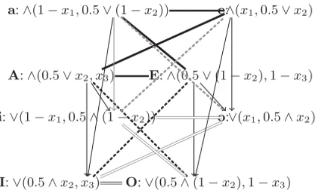
Example 1. We considerC = {1, 2, 3} and π1= 0, π2= 0.5 and π3= 1; see Fig. 4.
– on vertex A (resp. I) a fully satisfied object is such that x2= x3= 1 (resp. x3= 1).
– on vertex a (resp. i) a fully satisfied object is such that x1= x2= 0 (resp. x1= 0),
The operations of the front facet of the cube of Fig. 3 merge positive evaluations that focus on the high satisfaction of important criteria, while the local ratings xi on
the back could be interpreted as negative ones (measuring the intensity of faults). Then aggregations yield global ratings evaluating the lack of presence of important fault. In this case, weights are tolerance levels forbidding a fault to be too strongly present Then the vertices a and i in the back facet are interpreted differently: a is true if all somewhat intolerable faults are fully absent; i is true if there exists at least one intolerable fault that is absent. This framework this involves two complementary points of view, recently discussed in a multiple criteria aggregation perspective [6].
i: ∨(1 − x1,0.5 ∧ (1 − x2)) I: ∨(0.5 ∧ x2, x3) O: ∨(0.5 ∧ (1 − x2), 1 − x3) o:∨(x1,0.5 ∧ x2) a: ∧(1 − x1,0.5 ∨ (1 − x2)) A: ∧(0.5 ∨ x2, x3) E: ∧(0.5 ∨ (1 − x2), 1 − x3) e:∧(x1,0.5 ∨ x2)
Fig. 4. Cube of weighted qualitative aggregations
3
Sugeno integrals, desintegrals and rules
In the definition of Sugeno integral the relative weights of the set of properties are represented by a capacity (or fuzzy measure) which is a set function µ: 2C → L that
satisfies µ(∅) = 0, µ(C) = 1 and A ⊆ B implies µ(A) ≤ µ(B).
In order to translate a Sugeno integral into rules we also need the notions of conju-gate capacity, qualitative Moebius transform and focal sets: The conjuconju-gate capacity of µ is defined by µc(A) = 1 − µ(A) where A is the complementary of A.
In this paper, the capacities are supposed to be normalized in a special way, i.e. ∃A 6= C such that µ(A) = 1 and ∃B such that µc(B) = 1. It is worth noticing that in
such a context there exists a non-empty set, namely B, such that µ(B) = 0.
The inner qualitative Moebius transform of a capacity µ is a mapping µ#: 2C → L
defined by
µ#(E) = µ(E) if µ(E) > max
B⊂Eµ(B) and 0 otherwise.
It contains the minimal information characterizing µ (µ(A) = maxE⊆Aµ#(E)). A
set E for which µ#(E) > 0 is called a focal set. The set of the focal sets of µ is denoted
byF(µ). The Sugeno integral of an object x with respect to a capacity µ is originally defined by [12, 13]:
Sµ(x) = max
α∈Lmin(α, µ({i|xi≥ α})). (1)
There are two equivalent expressions used in this article: Sµ(x) = max
A∈F(µ)[min(µ(A), mini∈Axi)] =A∈F(µminc)
[max(µ(A), max
i∈A xi)]. (2)
The first expression in (2) is the generalisation of a normal disjunctive form from Boolean functions to lattice-valued ones. The second is the generalisation of a nor-mal conjunctive form. Clearly using the first form, Sµ(x) = 1 if and only if there is a
focal set E of µ for which µ(E) = 1 and xi = 1 for all i in E. Likewise, using the
second form Sµ(x) = 0 if and only if there is a focal set F of µcfor which µc(F ) = 1
and xi= 0 for all i in F . The Sugeno integral can then be expressed in terms of if-then
rules that facilitate the interpretation of the integral, when it has been derived from dat a (see [1] for more details).
Selection rules Each focal T of µ corresponds to the selection rule: If xi≥ µ(T ) for all i ∈ T then Sµ(x) ≥ µ(T ).
The objects selected by such rules are those satisfying to a sufficient extent all properties present in the focal set appearing in the rule.
Elimination rules Each focal set of the conjugate µcwith level µc(F ) corresponds to
the following elimination rule:
If xi≤ 1 − µc(F ) for all i ∈ F then Sµ(x) ≤ 1 − µc(F ).
The objects rejected by these rules are those that do not satisfy enough the proper-ties in the focal set of µcof some such rule.
When Sugeno integrals are used as aggregation functions for selecting acceptable objects, the properties are considered positive: the global evaluation increases with the partial ratings. But generally we have also negative properties: the global evaluation increases when the partial ratings decrease. In such a context we can use a desintegral associated to the Sugeno integral. We now presents this desintegral.
In the case of negative properties, weights are assigned to sets of properties by means of an anti-capacity (or anti-fuzzy measure) which is a set function ν : 2C → L
such that ν(∅) = 1, ν(C) = 0, and if A ⊆ B then ν(B) ≤ ν(A). Clearly, ν is an anticapacity if and only if1 − ν is a capacity. The conjugate νc of an anti-capacity ν
is an anti-capacity defined by νc(A) = 1 − ν(A), where A is the complementary of
A. The desintegral is defined from the corresponding Sugeno integral, by reversing the direction of the local value scales (x becomes1 − x), and by considering a capacity induced by the anti-capacity ν, as follows:
Sν↓(x) = S1−νc(1 − x). (3)
Based on this identity, we straightforwardly obtain the following rules associated to the desintegral S↓
ν from those derived from the integral S1−νc:
Proposition 1
Selection rules Each focalT of1 − νccorresponds to the selection rule:
Ifxi≤ νc(T ) for all i in T , then Sν↓(x) ≥ 1 − νc(T ).
The objects selected by these rules are those that do not possess, to a high extent
(less thanνc(T )), faults present in the focal set of the capacity 1 − νc.
Elimination rules Each focal set of1 − ν corresponds to the elimination rule:
Ifxi≥ 1 − ν(F ) for all i ∈ F then Sν↓(x) ≤ ν(F ).
The objects rejected by these rules are those possessing to a sufficiently large extent
the faults in the focal sets of the capacity1 − ν.
4
The cube of opposition and Sugeno integrals
When we consider a capacity µ, its pessimistic part is µ∗(A) = min(µ(A), µc(A)) and
its optimistic part is µ∗(A) = max(µ(A), µc(A)) [8]. We have µ
∗ ≤ µ∗, µ∗c = µ∗
and µ∗c = µ
∗. We need these notions in order to respect the fact that, in the square of
opposition, the vertices A, E express stronger properties than vertices I, O.
Proposition 2 A capacityµ induces the following square of opposition for the
associ-ated Sugeno integrals
A: Sµ∗(x) E: Sµ∗(1 − x)
I: Sµ∗(x) O: Sµ∗(1 − x)
Proof. Aentails I and E entails O since µ∗ ≤ µ∗. A and O (resp. E and I) are the
negation of each other since for all capacities µ we have the relation:
Sµ(x) = 1 − Sµc(1 − x). (4)
Let us prove that expressions at vertices A and E cannot be both equal to 1. Consider x such that Sµ∗(x) = 1, hence using Equation (4), 1 = 1 − Sµ∗(1 − x). So Sµ∗(1 − x) ≤
Sµ∗(1 − x) = 0 which entails Sµ
∗(1 − x) = 0.
Similarly we can prove that I and O cannot be false together.
Remark 1. In the above square of opposition, A and E can be false together and I and
O can be true together. For instance, if µ is a non-fully informed necessity measure N (for instanceF(N ) = {E}, with weight 1, where E is not a singleton), it comes down to the known fact that we can find a subset A such that N(A) = N (A) = 0, and for possibility measure Π(A) = 1 − N (A) it holds that Π(A) = Π(A) = 1.
Note that Sµ∗(1 − x) = S1−µ∗(x) and Sµ∗(1 − x) = S1−µ∗(x) where 1 − µ
∗
1 − µ∗are anti capacities. Hence a capacity µ defines a square of opposition where the
decision rules on the vertices A and I (resp.E and O) are based on a Sugeno integral (resp. desintegral).
In order to present the cube associated to Sugeno integrals we need to introduce the negation of a capacity µ, namely the capacity µ defined as follows: µ#(E) = µ#(E)
and µ(A) = maxE⊆Aµ#(E). A square of opposition aieo can be defined with the
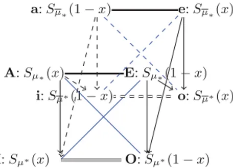
capacity µ. Hence we can construct a cube AIEO and aieo as follows: [9]:
i: Sµ∗(1 − x) I: Sµ∗(x) O: Sµ∗(1 − x) o: Sµ∗(x) a: Sµ∗(1 − x) A: Sµ∗(x) E: Sµ∗(1 − x) e: Sµ∗(x)
Proposition 3 If∃i 6= j ∈ C such that xi = 0, xj = 1 and {i}, {j}, C\{i}, C\{j} are
focal sets ofµ, then the cube in Fig. 5 is a cube of opposition.
Proof. AIEOand aieo are squares of opposition (due to µ∗≤ µ∗and µ∗≤ µ∗).
Let us prove that Sµ∗(x) ≤ Sµ∗(1 − x) (the arrow A → i on the left side facet).
Sµ∗(x) = minA[max(min(µ(A), 1 − µ(A)), maxi∈Axi] and
Sµ∗(1 − x) = maxA[min(max(µ(A), 1 − µ(A)), mini∈A(1 − xi)]. So we just need to
find sets E and F such that one term insideminAis less that one term insidemaxA.
Let us consider A= {i} where i is such that xi= 0. We have
max(min(µ(A), 1 − µ(A)), maxi∈Axi) = min(µ(C\{i}), 1 − µ({i})) and
min(max(µ(A), 1 − µ(A)), mini∈A(1 − xi)] = max(µ({i}), 1 − µ(C\{i})).
Note that µ(C\{i}) = µ#(C\{i}), since C\{i} is focal for µ and µ({i}) = µ#({i}) =
µ#(C\{i}) by definition. So min(µ(C\{i}), 1 − µ({i})) ≤ µ(C\{i}) = µ#(C\{i}) ≤
max(µ({i}), 1 − µ(C\{i})). The inequality Sµ∗(1 − x) ≤ Sµ∗(x) linking a with I, is
obtained, under the condition∃j ∈ C such that xj = 1, and C\{j} must be a focal set
of µ, i.e.,{j} is focal for µ using the equation (4). For arrow E → o and e → O, we need by symmetry to exchange i and j in the above requirements. This concludes the proof.
The cube of opposition is reduced to the facet AEIO if and only if µ= µ. So the cube is degenerated if and only if for each focal set T 6= C of µ, the complement T is also focal and µ#(T ) = µ#(T ), in other words, capacities expressing ignorance in the
sense that µ(A) = µ(A) for all A 6= ∅, C. Likewise the cube is reduced to the top facet AEea, if µ is self-conjugate, that is, µ= µc, i.e., µ(A) + µ(A) = 1.
5
Discussing aggregation attitudes with the cube
In this following, we characterize situations where objects get a global evaluation equal to1 using aggregations on the top facet. According to the selection rules, we can restrict to focal sets of the capacity with weight1.
Proposition 4 The global evaluations at vertices AIai of a cube associated to a
ca-pacityµ are maximal respectively in the following situations pertaining to the focal sets
ofµ:
A: The set of totally satisfied properties contain a focal set with weight 1 and
over-laps all other focal sets.
I: The set of satisfied properties contains a focal set with weight 1 or overlaps all
other focal sets.
a: The set of totally violated properties contains no focal set and its complement is
contained in a focal set with weight 1.
i: The set of totally violated properties contains no focal set or its complement is
contained in a focal set with weight 1.
Proof. A: Sµ∗(x) = 1 iff there exists a set A such that µ∗(A) = 1 and for all i in
A, xi= 1. µ∗(A) = 1 is equivalent to µ(A) = 1 and µc(A) = 1, that is µ(A) = 0.
I: Sµ∗(x) = 1 iff ∃A such that µ∗(A) = 1 and for all i in A, xi = 1. Since µ∗(A) =
max(µ(A), µc(A)) = 1, either µ(A) = 1 or µc(A) = 1, i.e., µ(A) = 0. So A
contains a focal set of µ with weight 1 or it overlaps all focal sets.
a: Sµ∗(1 − x) = 1 if and only if there exists a set A such that µ∗(A) = 1 and for all i
in A, xi = 0. The condition µ∗(A) = 1 reads µ(A) = 1 and µc(A) = 1. The first
condition says that µ#(B) = 1 for some subset B of A that is µ#(B) = 1, where
B contains A. The second condition says that µ(A) = 0 = µ(A). It means that there is no focal set of µ contained in A. So Sµ∗(1 − x) = 1 if and only if there
exists A such that for all i in A, xi = 0, and A is contained in a focal set of µ with
weight 1, and A contains no focal set of µ.
i: Sµ∗(1 − x) = 1 iff ∃A such that µ∗(A) = 1 and for all i in A, xi = 0. Since
µ∗(A) = max(µ(A), µc(A)) = 1, either µ(A) = 1 or µc(A) = 1, i.e., µ(A) = 0.
So, from the previous case we find that Sµ∗(1 − x) = 1 if and only if for all i in
A, xi = 0, and A is contained in a focal set of µ with weight 1, or A contains no
focal set of µ.
Example 2. AssumeC = {p, q, r}. We want to select objects with properties p and q
or p and r. Hence we haveFµ= {{p, q}, {p, r}} with µ#({p, q}) = µ#({p, r}) = 1.
We can calculate the useful capacities:
capacity{p} {q} {r} {p, q} {p, r} {q, r} {p, q, r} µ# 0 0 0 1 1 0 0 µ 0 0 0 1 1 0 1 µc 1 0 0 1 1 1 1 µc # 1 0 0 0 0 1 0 µ# 0 1 1 0 0 0 0 µ 0 1 1 1 1 1 1 µc# 0 0 0 0 0 1 0 µc 0 0 0 0 0 1 1 µc≥ µ so µ ∗= µ and µ∗= µc µ≥ µcso µ∗= µ and µ ∗= µc
Note that µ is a possibility measure.
The aggregation functions on the vertices are: A: Sµ(x) = max(min(xp, xq), min(xp, xr)) I:Sµc(x) = max(x p,min(xq, xr)) a:Sµc(1 − x) = min(1 − x q,1 − xr) i:Sµ(1 − x) = max(1 − xq,1 − xr).
Note that for vertex A, the two focal sets overlap so that the first condition of Propo-sition 4 is met when Sµ(x) = 1. For vertex I, one can see that Sµc(x) = 1 when x
p= 1
and{p} does overlap all focal sets of µ; the same occurs when xq = xr = 1. For
ver-tex a, Sµc(1 − x) = 1 when x
q = xr = 0, and note that the complement of {q, r}
is contained in a focal set of µ, while {q, r} contains no focal set of µ. For vertex i, Sµ(1 − x) = 1 when, xq = 0 or xr= 0, and clearly, neither {q} not {r} contain any
focal set of µ, but the complement of each of them is a focal set of µ.
6
Concluding remarks
This paper has shown how the structure of the cube of opposition extends from ordi-nary sets to weighted min- and max-based aggregations and more generally to Sugeno
integrals, which constitute a very important family of qualitative aggregation operators, which moreover have a logical reading. The cube exhausts all the possible aggregation attitudes. Moreover, as mentioned in Section 2, it is compatible with a bipolar view where we distinguish between desirable properties and rejected properties. It thus pro-vides a rich theoretical basis for multiple criteria aggregation.
References
1. D. Dubois, C. Durrieu, H. Prade, A. Rico, Y. Ferro. Extracting decision rules from qualitative data using Sugeno integral: a case study Proc. 13th Europ. Conf. on Symbolic and Quantitative Approaches to Reasoning under Uncertainty (ECSQARU’15), LNCS, Springer, 2015. 2. D. Dubois , H. Prade. Weighted minimum and maximum operations. An addendum to ‘A
review of fuzzy set aggregation connectives’. Information Sciences, 39, 205-210, 1986. 3. D. Dubois , H. Prade. An introduction to bipolar representations of information and
prefer-ence. Int. J. Intelligent Systems, 23 (8), 866-877, 2008.
4. D. Dubois, H. Prade. From Blanch´e’s hexagonal organization of concepts to formal concept analysis and possibility theory. Logica Univers., 2012, vol. 6, 149-169.
5. D. Dubois, H. Prade, A. Rico. Qualitative integrals and desintegrals - Towards a logical view. Proc. Int. Conf. on Modeling Decisions for Artificial Intelligence (MDAI’12), Springer, LNCS 7647, 127-138, 2012.
6. D. Dubois, H. Prade, A. Rico. Qualitative integrals and desintegrals: How to handle positive and negative scales in evaluation. Proc. 14th IPMU (Information Processing and Management of Uncertainty in Knowledge-Based Systems), vol. 299 of CCIS, Springer, 306-316, 2012 7. D. Dubois, H. Prade, A. Rico. The logical encoding of Sugeno integrals. Fuzzy Sets and
Systems, 241, 61-75, 2014.
8. D. Dubois, H. Prade, A. Rico. On the informational comparison of qualitative fuzzy measures. Proc. IPMU’14 (Information Processing and Management of Uncertainty in Knowledge-Based Systems), vol. 442 of CCIS, 216-225, 2014.
9. D. Dubois, H. Prade, A. Rico. The cube of opposition. A structure underlying many knowledge representation formalisms. Proc. 24th Int. Joint Conf. on Artificial Intelligence (IJCAI’15), Buenos Aires, Jul. 25-31, to appear, 2015.
10. T. Parsons. The traditional square of opposition. In: E. N. Zalta, editor, The Stanford Ency-clopedia of Philosophy. 2008.
11. H. Prade, A. Rico. Decribing acceptable objects by means of Sugeno integrals. in proc. In-ternational Conference on Soft Computing and Pattern Recognition (Socpar) p.6-11 (2010). 12. M. Sugeno. Theory of Fuzzy Integrals and its Applications, Ph.D. Thesis, Tokyo Institute of
Technology, Tokyo, 1974.
13. M. Sugeno. Fuzzy measures and fuzzy integrals: a survey. In: Fuzzy Automata and Decision Processes, (M.M. Gupta, G.N. Saridis, and B.R. Gaines, eds.), North-Holland, 89-102, 1977.