HAL Id: hal-03221512
https://hal.inria.fr/hal-03221512
Submitted on 8 May 2021HAL is a multi-disciplinary open access
archive for the deposit and dissemination of sci-entific research documents, whether they are pub-lished or not. The documents may come from teaching and research institutions in France or abroad, or from public or private research centers.
L’archive ouverte pluridisciplinaire HAL, est destinée au dépôt et à la diffusion de documents scientifiques de niveau recherche, publiés ou non, émanant des établissements d’enseignement et de recherche français ou étrangers, des laboratoires publics ou privés.
Experimental Comparison of Semi-parametric,
Parametric, and Machine Learning Methods for
Time-to-Event Analysis Through the IPEC Score
Camila Fernández, Chung Shue Chen, Pierre Gaillard, Alonso Silva
To cite this version:
Camila Fernández, Chung Shue Chen, Pierre Gaillard, Alonso Silva. Experimental Comparison of Semi-parametric, Parametric, and Machine Learning Methods for Time-to-Event Analysis Through the IPEC Score. SFdS 2020 - 52èmes Journées de Statistiques de la Société Française de Statistique, Jun 2021, Nice, France. pp.1-6. �hal-03221512�
Experimental Comparison of Semi-parametric,
Parametric, and Machine Learning Methods for
Time-to-Event Analysis Through the IPEC Score
Camila Fern´andez1,2, Chung Shue Chen2, Pierre Gaillard3, Alonso Silva4 1Sorbonne Universit´e, 2Nokia Bell Labs, 3INRIA, 4Safran Tech
{camila.fernandez, chung shue.chen}@nokia.com, [email protected], [email protected]
Abstract. In this paper, we make an experimental comparison of semi-parametric (Cox proportional hazards model, Aalen additive model), parametric (Weibull AFT model), and machine learning methods (Random Survival Forest, Gradient Boosting Cox propor-tional hazards loss, DeepSurv) through the IPEC score on three different datasets (PBC, GBCSG2 and TLCM).
Keywords. Machine Learning, Survival Analysis, Health, Bootstrap, IPEC score. Acknowledgment. The work presented here has been partially carried out at LINCS.
1
Introduction
Time-to-event analysis is a branch of statistics that looks for modeling the time remaining until a certain critical event occurs. For example, this event can be the time until a biological organism dies or the time until a machine fails. There are many other examples, in healthcare, the aim is usually to predict the time until a patient with certain disease dies or the time until the recurrence of an illness, whereas in telecom, the goal could be to predict the customer churn, etc. One of the main interests of time-to-event analysis is right censoring, it comes naturally from the fact that not necessary all the samples have reached the event time which makes the problem more difficult and a different challenge from the typical regression problem.
In Fernandez et all. (2020), the performance (through the concordance index) of several models have been compared on two different datasets, both of them related to a healthcare approach. The first one is about patients diagnosed with primary biliary cirrhosis (PBC) where the goal is to predict the time until the patient dies. The second dataset consists on patient diagnosed with breast cancer and the objective is to predict the recurrence of the disease. Here we add a third dataset which is from a different source, it consists on clients from a telecommunication company, Telco (TLCM), and the aim is to predict the customer churn. We also consider a different score to carry out this comparison, the IPEC score (see Section 1.2).
In this work, we implement a bootstrapping technique for the computation of the IPEC score in the test set, this is with the aim of obtain a better approximation of the asymptotic behavior of the estimated event time. Each sample of each dataset has an
observed time which can correspond either to a survival time or a censored time. A censored time will be a lower bound for the survival time and so we will be in the case in which the critical event has not occurred at the moment of the observation.
Survival and hazard function The fundamental task of time-to-event analysis is to estimate the probability distribution of time until some event of interest happens.
Consider a covariates/features vector X, a random variable that takes on values in the covariates/features space X . Consider a survival time T , a non-negative real-valued random variable. Then, for a feature vector x ∈ X , our aim is to estimate the conditional survival function:
S(t|x) := P(T > t|X = x), (1) where t ≥ 0 is the time and P is the probability function. In order to estimate the conditional survival function S(·|x), we assume that we have access to a certain dataset in which for the i-th sample we have: Xi the feature vector, δi the survival time indicator,
which indicates whether we observe the survival time or the censoring time, and Yi which
is the survival time if δi = 1 and the censoring time otherwise. We split the dataset into
a training set of size n and a test set of size m. The training set is used to estimate the parameters of each model and the test set to measure how accurate is the estimation of the probability function.
Many models have been proposed to estimate the conditional survival function S(·|x) such as Cox proportional hazards from Cox (1972), gradient boosting from Friedman (2001) and random survival forest from Ishwaran (2008). The most standard approaches are the semi-parametric and parametric models, which assume a given structure of the hazard function h(t|x) := −∂t∂ log S(t|x).
IPEC score The IPEC score, introduced first by Gerds and Schummacher (2006), is an alternative score to the concordance index that we used in a previous work in Fernandez et all. (2020) in order to measure the accuracy of time to event models. The IPEC score is a consistent estimator for the mean square error of the probability function S. We used a variant of the original IPEC score which was presented by Chen (2019). This score approximates the following MSE of a survival probability estimator ˆS, which cannot be directly computed from the dataset,
M SE( ˆS) = Z τ
0
E[(1{T > t} −S(t|X))ˆ 2]dt (2) where τ is a user-specified time horizon and T is the survival time of feature vector X. Let us define SC(t|x) = P(C > t|X = x) where C is the censored time. Then, the IPEC
score is computed as follows. Let ˆSC be an estimator of SC,
IP EC( ˆS) = 1 m m X i=1 Z τ 0 Wi(t)(1{Yi > t) − ˆS(t|Xi))2 (3)
where (Xi, Yi, δi) for 0 < i ≤ m are the samples of the test set. Wi is defined as: Wi(t) = (δ i1{Yi≤t} ˆ SC(Yi|Xi) + 1{Yi>t} ˆ SC(t|Xi) ˆ SC(t|Xi) ≥ θ 1/θ otherwise. (4)
Here, θ is an user-specified bound which was introduced in order to prevent a division by 0 and then, in the worst case, the IPEC score is finite. The addition of this last parameter is the only difference between the original IPEC score of Gerds and Schum-macher (2006) and the variant introduced by Chen (2019). In practice, θ can be set as an arbitrarily small but positive constant. Note that 0 ≤ IP EC( ˆS) ≤ τ /θ.
2
Datasets Description
German Breast Cancer Study Group dataset (GBCSG2) The German Breast Cancer Study Group (GBCSG2) dataset, made available by Schumacher et al. (1994), studies the effects of hormone treatment on recurrence-free survival time. The event of interest is the recurrence of cancer time. The dataset has 686 samples and 8 co-variates/features: age, estrogen receptor, hormonal therapy, menopausal status (pre-menopausal or post(pre-menopausal), number of positive nodes, progesterone receptor, tumor grade, and tumor size. At the end of the study, there were 387 patients (56.4%) who were right censored (recurrence-free).
Mayo Clinic Primary Biliary Cirrhosis dataset (PBC) The Mayo Clinic Primary Biliary Cirrhosis dataset, made available by Therneau and Grambsch (2000), studies the effects of the drug D-penicillamine on the survival time. The event of interest is the death time. The dataset has 276 samples and 17 covariates/features: age, serum albumin, alkaline phosphatase, presence of ascites, aspartate aminotransferase, serum bilirunbin, serum cholesterol, urine copper, edema, presence of hepatomegaly or enlarged liver, case number, platelet count, standardized blood clotting time, sex, blood vessel malformations in the skin, histologic stage of disease, treatment and triglycerides. At the end of the study, there were 165 patients (59.8%) who were right censored (alive).
Kaggle Telco Churn (TLCM) The Kaggle Telco Churn dataset, made available by Kaggle in 2008, studies the possible causes of customer churn in a telecommunication enterprise. The event of interest is the churn time of the clients. The dataset has 7043 samples and 19 covariates/features: customer ID, gender, senior citizen, partner, depen-dents, phone service, multiple lines, internet service, online security, online backup, device protection, tech support, streaming TV, streaming movies, contract, paperless billing, payment method, monthly charges and total charges. At the end of the study, there were 5174 clients (73%) who were right censored (not have churned yet).
3
Models
We took into consideration several models for the comparison analysis. Semi-parametric models such as Cox (1972) and Aalen’s additive (1989), both models assume certain parametrical structure on the hazard function. These models are semi-parametric in the sense that the baseline hazard function does not have to be specified and it can vary allowing a different parameter to be used for each unique survival time.
We also consider a parametric model, Weibull accelerated failure time by Liu (2018), it supposes that the hazard function depends on an accelerated rate λ(x) which can be estimated parametrically.
Finally we consider machine learning models such as Random survival forest proposed by Ishwaran et all. (2008), Gradient boosting cox proportional hazards loss proposed by Friedman (2001), DeepSurv by Katzman et all. (2018) and a variation of random survival forest proposed by Chen (2019). We also considered a randomized search of the parameters which was done by cross validation. For more information and details about these models look at Fernandez et all. (2020).
4
Results and Conclusion
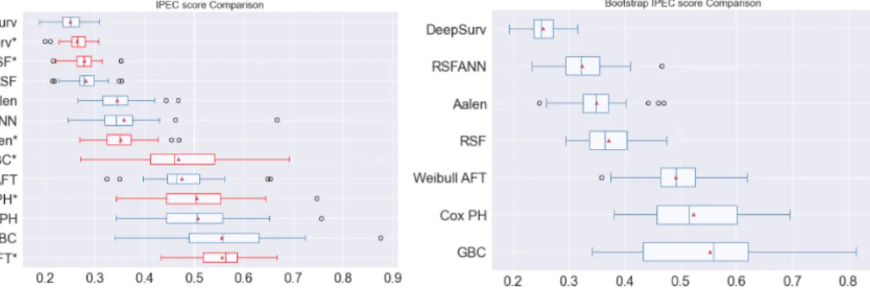
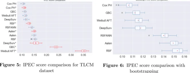
For each dataset, we choose 25 different seeds for splitting the data which generates 25 different partitions between training and test sets (75% and 25% respectively). We repeat the experiment 25 times and we make a boxplot with the distribution of the IPEC scores obtained. Fig. 1, 3 and 5 respectively compare the IPEC score for PBC, GBCSG2 and TLCM datasets, and Fig. 2, 4 and 6 show the same comparison after re-sampling the test set five times (bootstrapping).
In Fig. 1, we can appreciate that Gradient boosting with randomized search of the parameters performs better than the other models and DeepSurv is in second place. Fig. 3 shows that DeepSurv outperforms all the other models for GBCSG2. And finally, Fig. 5 shows the comparison for TLCM dataset where we can observe that Cox proportional Hazards model is the model with the best performance and DeepSurv dropped down to the fifth place.
Furthermore, we can observe that traditional methods performed reasonably well for the big dataset TLCM, but they underperformed against machine learning methods for the smaller datasets (GBCSG2 and PBC). We can also observe that the deep learning method (Deepsurv) performed better than random survival forest model in all the datasets.
Fig. 2, 4 and 6 show the comparison of the IPEC score using the bootstrapping tech-nique. We appreciate that DeepSurv outperforms all the other models for the smaller datasets (PBC and GBCSG2) and Cox proportional hazards has the best result for the biggest dataset (TLCM) as in the previous case without re-sampling.
This shows that there is no much difference in the results when we apply the bootstrap-ping technique for the test of the models. In addition, we know that classical methods
are easier to interpret in the sense of measure how each covariate/feature influences in the model. For the case of PBC dataset, gradient boosting with random search outperforms DeepSurv by a 12% while similarly in TLCM the method cox proportional hazards in-crease the performance by a 12% with respect to Deepsurv model. The case of GBCSG2 is different because DeepSurv improves the performance in a 37% compared to Aalen’s additive method, therefore, if this increment of performance is significant enough to com-pensate the loss of interpretation will depend mainly on the applications.
Figure 1: IPEC score comparison for PBC dataset
Figure 2: IPEC score comparison with bootstrapping
Figure 3: IPEC score comparison for GBCSG2 dataset
Figure 4: IPEC score comparison with bootstrapping
Figure 5: IPEC score comparison for TLCM dataset
Figure 6: IPEC score comparison with bootstrapping
Bibliographie
Aalen, O. O. (1989). A linear regression model for the analysis of life times. Statistics in Medicine, vol. 8, pp. 907–925.
Chen, G. (2019). Nearest neighbor and kernel survival analysis: Nonasymptotic error bounds and strong consistency rates. arXiv preprint arXiv:1905.05285.
Cox, D. R. (1972). Regression models and life-tables. Journal of the Royal Statistical Society, Series B. 34 (2): 187–220.
Davidson-Pilon, C., et al. (2020), CamDavidsonPilon/lifelines:v0.23.9, doi: 10.5281/zen-odo.805993.
Efron, B. (1982), The jacknife, the bootstrap and other resampling plans, SIAM.
Fern´andez, C., Chen, C. S., Gaillard, P., Silva, A. (2020), Experimental comparison of semi-parametric, parametric and machine learning models for time-to-event analysis through the concordance index. Journ´ee de Statistique SFdS, pp.317-325
Friedman, J. H. (2001). Greedy function approximation: A gradient boosting machine. Annals of Statistics, pp.1189-1232
Ishwaran, H., Kogalur, U. B., Blackstone, E. H., Lauer, M. S. (2008). Random survival forests. Annals of Applied Statistics, vol. 2, no. 3, pp. 841–860.
Katzman J., et al. (2018). DeepSurv: Personalized treatment recommender system using a Cox proportional hazards deep neural network. BMC Medical Research Methodology. Pedregosa, F., et al. (2011). Scikit-learn: Machine learning in Python, JMLR.
P¨olsterl, S. (2019). Scikit-survival:v0.11, doi:10.5281/zenodo.3352342.
Schumacher, M., et al. (1994), Randomized 2 x 2 trial evaluating hormonal treatment and the duration of chemotherapy in node-positive breast cancer patients. Journal of Clinical Oncology, 12(10), pp. 2086–2093.
Liu, E. (2018), Using Weibull accelerated failure time regression model to predict survival time and life expectancy. BioRxiv.