Contribution à l’inspection automatique des pièces flexibles à l'état libre sans gabarit de conformation

(1)

(2)

UNIVERSITÉ DU QUÉBEC

DOCTORAT PRÉSENTÉ À

L’UNIVERSITÉ DU QUÉBEC À TROIS-RIVIÈRES COMME EXIGENCE PARTIELLE

DU DOCTORAT EN INGÉNIERIE OFFERT EN EXTENSION

EN VERTU D’UN PROTOCOLE D’ENTENTE AVEC L’UNIVERSITÉ DU QUÉBEC À CHICOUTIMI

PAR

Sasan Sattarpanah Karganroudi

CONTRIBUTION À L’INSPECTION AUTOMATIQUE DES PIÈCES FLEXIBLES À L'ÉTAT LIBRE SANS GABARIT DE CONFORMATION

(3)

DO C TO R AT EN INGÉNIERIE (PH. D.)

Programme offert par l’Université du Québec à Chicoutimi (UQAC)

en extension avec

l’Université du Québec à Trois-Rivières (UQTR)

Cette thèse a été dirigée par :

Vincent François, directeur de recherche, PhD Université du Québec à Trois-Rivières

Jean-Christophe Cuillière, codirecteur de recherche, PhD Université du Québec à Trois-Rivières

Jury d’évaluation de la thèse :

Luc Laperrière, PhD. Université du Québec à Trois-Rivières

René Mayer, PhD. École Polytechnique de Montréal

Louis Rivest, PhD. École de Technologie Supérieure

(4)

RÉSUMÉ

Le marché industriel compétitif exige une production de haute qualité de la part des compagnies de fabrication. Le département de contrôle qualité dans les secteurs industriels vérifie les exigences géométriques des produits en se référant aux tolérances. Ces exigences sont présentées dans les normes de Dimensionnement Géométrique Et Tolerances (DG&T). Toutefois, les méthodes conventionnelles de mesure et de dimensionnement sont couteuses et longues. De nos jours, les méthodes de mesure manuelles sont remplacées par les méthodes automatisées dites Inspection Assistée par Ordinateur (IAO). Les méthodes IAO appliquent les améliorations dans le calcul informatique et les dispositifs d’acquisition de données 3-D afin de comparer le maillage du modèle scanné de la pièce fabriquée avec le modèle conçu par ordinateur utilisant la Conception Assistée par Ordinateur (CAO). Les normes de métrologie, telles que ASME-Y14.5 et ISO-GPS, exigent la mise en œuvre de l'inspection à l'état libre dans lequel la pièce est soumise uniquement à la gravité. Les pièces souples (non rigide) sont exemptées de la règle d'inspection à l'état libre en raison de l'écart géométrique significatif de ces dernières au dit-état tenant compte des tolérances. En dépit du développement des méthodes IAO, l’inspection des pièces souples demeure un sérieux défi. Les méthodes d'inspection conventionnelles appliquent des gabarits complexes pour récupérer la forme fonctionnelle des pièces souples. Cependant, la fabrication et la configuration de ces gabarits de conformité sont compliquées et chères. Depuis que les clients et les industriels exigent des gabarits d’inspection répétitifs et indépendants, le prix de ces derniers a doublé. Les méthodes d'inspection sans gabarit des pièces souples basées sur les méthodes IAO ont été développées afin d'éliminer l’utilisation couteuse des gabarits de conformité. Ces procédés visent à distinguer les déformations flexibles des pièces à l'état libre des défauts. Les méthodes d'inspection sans gabarits doivent être automatiques, fiables, précises et reproductibles pour les pièces souples aux formes sophistiquées. Le modèle scanné, qui est obtenu sous forme de nuages de points, représente la forme d'une pièce à l'état libre. Ensuite, l'inspection des défauts est réalisée en comparant les modèles scannés

(5)

et CAO, mais ces modèles sont présentés dans des systèmes de coordonnées indépendants. En effet, le modèle scanné est présenté dans le système de coordonnées du système de mesure (système de numérisation) tandis que le modèle de CAO est dans le système de coordonnées de conception. Pour effectuer l'inspection et faciliter une comparaison précise entre les modèles, le processus de recalage est nécessaire afin d’aligner et ramener plus près les modèles scanné et CAO dans un système commun de coordonnées. Le recalage inclut une compensation virtuelle de la déformation flexible des pièces à l'état libre. Après, l’inspection est assurée par une comparaison géométrique entre les modèles CAO et les pièces souples scannées.

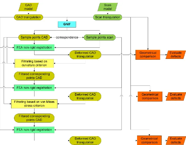
La présente thèse porte sur l’élaboration de méthodes automatiques d'inspection assistée par ordinateur sans gabarit. Ceci constitue une amélioration de la méthode d'inspection numérique généralisée (Generalized Numerical Inspection Fixture (GNIF)). Cette thèse présente également la vérification de la robustesse de notre nouvelle méthode. À cet effet, une méthode IAO automatique et sans gabarit pour des pièces souples basée sur des points de correspondance a été développée afin d’identifier et de quantifier plus précisément les défauts sur la surface des modèles scannés. La déformation flexible des pièces à l'état libre dans notre méthode est compensée en appliquant le recalage basé sur la méthode d’éléments finis, Recalage Non rigide par Élément Finis (RNÉF), pour déformer le modèle CAO vers le maillage du modèle scanné. Des points d'échantillonnage correspondants générés entre les modèles CAO et scanné d'une pièce sont utilisés afin de calculer le champ de déplacement qui sert de conditions aux limites dans RNÉF. Ces points d'échantillonnage correspondants, qui sont générés par la méthode GNIF, sont répartis uniformément sur la surface des modèles. La comparaison entre ce modèle CAO déformé et le maillage du modèle scanné vise à évaluer et à quantifier les défauts sur le modèle scanné. Cependant, certains points d'échantillonnage peuvent être situés à proximité ou sur des zones défectueuses, ce qui entraîne une estimation inexacte des défauts. Ces points d'échantillonnage sont automatiquement filtrés dans cette méthode IAO basée sur le calcul d’estimation de courbure et les contraintes de von Mises. Une fois filtrés, les points d'échantillonnage restants sont utilisés dans un nouveau RNÉF, ce qui

(6)

permet une évaluation précise des défauts par rapport aux tolérances. Toutes les méthodes d’IAO nécessitent une évaluation de la performance et de la robustesse de la méthode par rapport aux mesures actuelles. Cette thèse introduit également une nouvelle métrique de validation pour la vérification et la validation (V&V) des méthodes IAO basée sur les recommandations ASME. L'approche V&V développée utilise un test d'hypothèse statistique non paramétrique, à savoir le test de Kolmogorov-Smirnov (K-S). En plus de valider la taille des défauts, le test K-S permet une évaluation plus approfondie basée sur la répartition de la distance entre le modèle scanné et le modèle CAO pour chaque défaut. La robustesse de notre méthode IAO par rapport aux incertitudes telles que les bruits de scan est évaluée quantitativement en utilisant la métrique de validation développée. En raison de la conformité des pièces souples, une pièce ayant des défauts peut encore être assemblée à l'état d'assemblage. Cette thèse présente également une méthode originale d’IAO sans gabarit pour des pièces souples comportant des défauts afin d’évaluer la faisabilité de l'assemblage de ces pièces à l'état d'assemblage fonctionnel. Notre méthode d'inspection virtuelle de montage à l'état d'assemblage, Virtual Mounting Assembly-State Inspection (VMASI), effectue un recalage non rigide pour monter virtuellement le maillage du modèle scanné à l'état d'assemblage. À cet effet, les nuages de points du modèle scanné représentant la pièce à l'état libre sont déformés pour répondre aux contraintes d'assemblage telles que la position de fixation (par exemple des trous de montage). Pour atteindre les exigences fonctionnelles sur des pièces souples comportant des défauts, l'application de charges d'assemblage est autorisée à la surface du modèle scanné. Ces charges d'assemblage sont limitées aux charges admissibles. Les charges d'assemblage requises sont estimées grâce à une nouvelle méthode d’optimisation de calcul des pressions de montage (pour mise en forme de la pièce sur le gabarit virtuel), Restraining Pressures Optimization (RPO), visant à déplacer le modèle scanné afin d'atteindre la tolérance pour les trous de montage. Par conséquent, le modèle scanné ayant des défauts peut être mis en forme sur le gabarit virtuel si les trous de montage sur la forme fonctionnelle prédite du modèle scanné atteignent la plage de tolérance. Différentes pièces de l'industrie aérospatiale sont utilisées pour évaluer la performance de nos

(7)

méthodes développées dans cette thèse. L'inspection automatique pour identifier les différents types de défauts au niveau local et général sur les pièces conduit à une évaluation précise des défauts. La robustesse de la méthode d'inspection est également testée avec différents niveaux de bruits de numérisation, ce qui présente des résultats prometteurs. La méthode VMASI est validée par différents types de pièces déformables (flexible) en aérospatiale. Nous concluons que certaines pièces comportant des défauts peuvent être mise en forme à l’état d'assemblage lorsqu’elles sont soumises à des charges admissibles.

Mots clés : Pièces souples, DG&T, Inspection Assistée par Ordinateur (IAO), méthode

d’éléments finis, inspection sans gabarit, recalage non rigide, état d’assemblage, état libre, montage virtuel, optimisation, vérification et validation (V&V).

(8)

ABSTRACT

The competitive industrial market demands manufacturing companies to provide the markets with a higher quality of production. The quality control department in industrial sectors verifies geometrical requirements of products with consistent tolerances. These requirements are presented in Geometric Dimensioning and Tolerancing (GD&T) standards. However, conventional measuring and dimensioning methods for manufactured parts are time-consuming and costly. Nowadays manual and tactile measuring methods have been replaced by Computer-Aided Inspection (CAI) methods. The CAI methods apply improvements in computational calculations and 3-D data acquisition devices (scanners) to compare the scan mesh of manufactured parts with the Computer-Aided Design (CAD) model. Metrology standards, such as ASME-Y14.5 and ISO-GPS, require implementing the inspection in free-state, wherein the part is only under its weight. Non-rigid parts are exempted from the free-state inspection rule because of their significant geometrical deviation in a free-state with respect to the tolerances. Despite the developments in CAI methods, inspection of non-rigid parts still remains a serious challenge. Conventional inspection methods apply complex fixtures for non-rigid parts to retrieve the functional shape of these parts on physical fixtures; however, the fabrication and setup of these fixtures are sophisticated and expensive. The cost of fixtures has doubled since the client and manufacturing sectors require repetitive and independent inspection fixtures. To eliminate the need for costly and time-consuming inspection fixtures, fixtureless inspection methods of non-rigid parts based on CAI methods have been developed. These methods aim at distinguishing flexible deformations of parts in a free-state from defects. Fixtureless inspection methods are required to be automatic, reliable, reasonably accurate and repeatable for non-rigid parts with complex shapes. The scan model, which is acquired as point clouds, represent the shape of a part in a free-state. Afterward, the inspection of defects is performed by comparing the scan and CAD models, but these models are presented in different coordinate systems. Indeed, the scan model is presented in the measurement coordinate system whereas the CAD model is introduced in the designed coordinate system. To accomplish the inspection and

(9)

facilitate an accurate comparison between the models, the registration process is required to align the scan and CAD models in a common coordinate system. The registration includes a virtual compensation for the flexible deformation of the parts in a free-state. Then, the inspection is implemented as a geometrical comparison between the CAD and scan models.

This thesis focuses on developing automatic and accurate fixtureless CAI methods for non-rigid parts along with assessing the robustness of the methods. To this end, an automatic fixtureless CAI method for non-rigid parts based on filtering registration points is developed to identify and quantify defects more accurately on the surface of scan models. The flexible deformation of parts in a free-state in our developed automatic fixtureless CAI method is compensated by applying FE non-rigid Registration (FENR) to deform the CAD model towards the scan mesh. The displacement boundary conditions (BCs) for FENR are determined based on the corresponding sample points, which are generated by the Generalized Numerical Inspection Fixture (GNIF) method on the CAD and scan models. These corresponding sample points are evenly distributed on the surface of the models. The comparison between this deformed CAD model and the scan mesh intend to evaluate and quantify the defects on the scan model. However, some sample points can be located close or on defect areas which result in an inaccurate estimation of defects. These sample points are automatically filtered out in our CAI method based on curvature and von Mises stress criteria. Once filtered out, the remaining sample points are used in a new FENR, which allows an accurate evaluation of defects with respect to the tolerances.

The performance and robustness of all CAI methods are generally required to be assessed with respect to the actual measurements. This thesis also introduces a new validation metric for Verification and Validation (V&V) of CAI methods based on ASME recommendations. The developed V&V approach uses a nonparametric statistical hypothesis test, namely the Kolmogorov–Smirnov (K-S) test. In addition to validating the defects size, the K-S test allows a deeper evaluation based on distance distribution of

(10)

defects. The robustness of CAI method with respect to uncertainties such as scanning noise is quantitatively assessed using the developed validation metric.

Due to the compliance of non-rigid parts, a geometrically deviated part can still be assembled in the assembly-state. This thesis also presents a fixtureless CAI method for geometrically deviated (presenting defects) non-rigid parts to evaluate the feasibility of mounting these parts in the functional assembly-state. Our developed Virtual Mounting Assembly-State Inspection (VMASI) method performs a non-rigid registration to virtually mount the scan mesh in assembly-state. To this end, the point clouds of scan model representing the part in a free-state is deformed to meet the assembly constraints such as fixation position (e.g. mounting holes). In some cases, the functional shape of a deviated part can be retrieved by applying assembly loads, which are limited to permissible loads, on the surface of the part. The required assembly loads are estimated through our developed Restraining Pressures Optimization (RPO) aiming at displacing the deviated scan model to achieve the tolerance for mounting holes. Therefore, the deviated scan model can be assembled if the mounting holes on the predicted functional shape of scan model attain the tolerance range.

Different industrial parts are used to evaluate the performance of our developed methods in this thesis. The automatic inspection for identifying different types of small (local) and big (global) defects on the parts results in an accurate evaluation of defects. The robustness of this inspection method is also validated with respect to different levels of scanning noise, which shows promising results. Meanwhile, the VMASI method is performed on various parts with different types of defects, which concludes that in some cases the functional shape of deviated parts can be retrieved by mounting them on a virtual fixture in assembly-state under restraining loads.

Keywords: non-rigid parts, Computer-Aided Inspection (CAI), GD&T, FEA, non-rigid

registration, fixtureless inspection, free-state, assembly-state, virtual mounting, optimization, verification and validation (V&V).

(11)

DEDICATION

(12)

ACKNOWLEDGMENTS

I express my deepest gratitude to my supervisors Professor Jean-Christophe Cuillière and Professor Vincent François for their support and precious advice during the research work.

I would like to extend my appreciation to Professor Souheil-Antoine Tahan from École de Technologie Supérieure (ÉTS) for his guidance and support during the course of this project.

I acknowledge Mr. Vahid Sabri from École de Technologie Supérieure (ÉTS) for his collaborations associated with the case studies and the GNIF method. I also acknowledge Mr. Vincent Mathon for his help towards nonlinear FEA simulation that is performed in the framework of his internship at Université du Québec à Trois-Rivières (UQTR). I thank all my colleagues in the laboratory of Équipe de Recherche en Intégration Cao-CAlcul (ÉRICCA) and my friends in UQTR for the four years of support and cooperation. The support and financial contribution of the Natural Sciences and Engineering Research Council of Canada (NSERC), Consortium for Aerospace Research and Innovation in Québec (CRIAQ), Mitacs and UQTR foundation is very much appreciated.

My great thanks go to my family and all my teachers for their unwavering support during the years of my studies.

(13)

LIST OF TABLES

Table 2-1: The classification for compliant behavior of parts concerning the induced displacement under applied force (Abenhaim, Desrochers et al. 2012). ... 44 Table 4-1: Estimated size of defects and errors based on curvature and von Mises criteria for Part A with small (local) defects and bending deformation. ... 101 Table 4-2: Estimated size of defects and errors based on curvature and von Mises criteria for part A with small (local) defects and torsion deformation. ... 111 Table 4-3: Estimated size of defects and errors based on curvature and von Mises criteria for Part A with a big (global) defect and bending deformation. ... 115 Table 4-4: Estimated size of defects and errors based on curvature and von Mises criteria for Part A with a big (global) defect and torsion deformation. ... 119 Table 4-5: Estimated size of defects and errors based on curvature and von Mises criteria for Part B with small (local) defects and bending deformation. ... 124 Table 4-6: Estimated size of defects and errors based on curvature and von Mises criteria for Part B with small (local) defects and torsion deformation. ... 127 Table 4-7: Estimated size of defects and errors based on curvature and von Mises criteria for Part B with a big (global) defect and bending deformation. ... 130 Table 4-8: Estimated size of defects and errors based on curvature and von Mises criteria for Part B with a big (global) defect and torsion deformation. ... 132 Table 5-1: Estimated size of defects and errors for part A with small (local) defects and bending deformation. ... 163 Table 5-2: Validation results with K-S tests (𝐻0: the distance distribution of nominal and estimated defects are sufficiently similar) at 5% significance level for part A with small (local) defects and bending deformation. ... 164 Table 5-3: Estimated size of defects and errors for part A with a big (global) defect and bending deformation. ... 166

(19)

Table 5-4: Validation results with K-S tests (𝐻0: the distance distribution of nominal and estimated defects are sufficiently similar) at 5% significance level for part A with a big (global) defect and bending deformation. ... 167 Table 5-5: Estimated size of defects and errors for part B with small (local) defects and bending deformation. ... 171 Table 5-6: Estimated size of defects and errors for part B with small (local) defects and torsion deformation. ... 174 Table 5-7: Validation results with K-S tests (𝐻0: the distance distribution of nominal and estimated defects are sufficiently similar) at 5% significance level for part B with small (local) defects under bending and torsion deformation. ... 175 Table 5-8: Estimated size of defects and errors for part B with a big (global) defect and bending deformation. ... 177 Table 5-9: Estimated size of defects and errors for part B with a big (global) defect and torsion deformation. ... 179 Table 5-10: Validation results with K-S tests (𝐻0: the distance distribution of nominal and estimated defects are sufficiently similar) at 5% significance level for part B with a big (global) defect and under bending and torsion deformation. ... 180 Table 5-11: Estimated size of defects and errors for part A with small (local) defects and large bending deformation. ... 184 Table 5-12: Validation results with K-S tests (𝐻0: the distance distribution of nominal and estimated defects are sufficiently similar) at 5% significance level for part A with small (local) defects and large bending deformation. ... 185 Table 5-13: Estimated size of defects and errors for part A with a big (global) defect and large bending deformation. ... 187 Table 6-1: Synthesis of validation cases defects for part A. ... 225 Table 6-2: Assembly pressure and force results for the validation case A-1. ... 227

(20)

Table 6-3: Position, profile and orientation results for the validation case A-1. ... 227

Table 6-4: Assembly pressure and force results for the validation case A-2. ... 229

Table 6-12: Assembly pressure and force results for the validation case of part B simulated as a small plastic defect. ... 239

Table 6-13: Position, profile and orientation results for the validation case of part B simulated as a small plastic defect. ... 239

Table 6-14: Assembly pressure and force results for the validation case of part B simulated as an intermediate plastic defect. ... 242

Table 6-15: Position, profile and orientation results for the validation case of part B simulated as an intermediate plastic defect. ... 242

Table 6-16: Assembly pressure and force results for the validation case of part B simulated as a large plastic defect. ... 245

Table 6-17: Position, profile and orientation results for the validation case of part B simulated as a large plastic defect. ... 245

Table 7-1: Estimated size of defects and errors implementing nonlinear and linear FENR. ... 260

(21)

LIST OF FIGURES

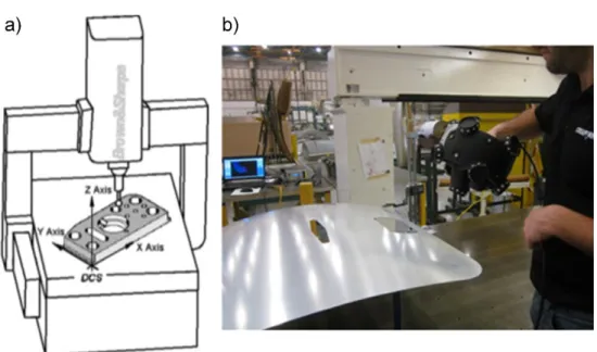
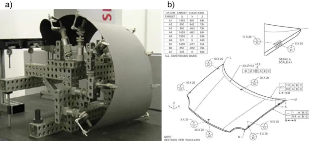
Figure 1-1: An ordinary aerospace panel, a) in free-state, b) constrained on supports of the inspection fixture (Abenhaim, Desrochers et al. 2015) ... 37 Figure 1-2: An aerospace panel restrained under known loads by using weights (the black sandbags) on its surface (Abenhaim, Desrochers et al. 2015). ... 38 Figure 1-3: Structure of the thesis based on the articles. ... 41 Figure 2-1: Classification of the compliant behavior of parts (Abenhaim, Desrochers et al. 2012)... 44 Figure 2-2: Measuring tools, a) using CMM for measuring a rigid part (Li and Gu 2004), b) using a noncontact scanner for scanning the surface of a non-rigid part. ... 46 Figure 2-3: Categorization of the quality requirements specifications for GD&T of

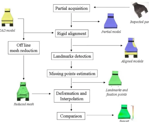
non-rigid parts (Abenhaim, Desrochers et al. 2012). ... 48 Figure 2-4: The restrained conditions for non-rigid parts, a) an inspection fixture restraining a curved aerospace panel (Ascione and Polini 2010) b) A non-rigid part restrained to the design shape using datum targets (ASME Y14.5). ... 49 Figure 2-5: The process chain of the virtual distortion compensation method (Weckenmann and Weickmann 2006). ... 54 Figure 2-6: Schematic flowchart of proposed virtual fixture method in (Abenhaim, Desrochers et al. 2015). ... 56 Figure 2-7: An overview of the non-rigid CAI method using partial measuring data (Jaramillo, Prieto et al. 2013). ... 58 Figure 2-8: constructing deformed CAD model using displacement field without taking into consideration the presence of effects (Abenhaim, Tahan et al. 2011). ... 59 Figure 2-9: Distance preserving property of non-rigid part during an isometric deformation (Radvar-Esfahlan and Tahan 2014). ... 61

(22)

Figure 2-10: Corresponding sample points (black points) generated on the CAD and scan models for a turbine blade (Radvar-Esfahlan and Tahan 2014). ... 62 Figure 2-11: The flowchart of the inspection process using GNIF method

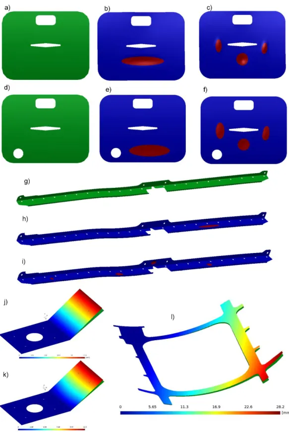
(Radvar-Esfahlan and Tahan 2012) ... 62 Figure 2-12: verification and validation (V&V) activities and results based on ASME recommendation (Schwer, Mair et al. 2012). ... 66 Figure 3-1: A complex inspection fixture set-up for a large aerospace panel. ... 70 Figure 3-2: simplified flowchart of a fixtureless CAI followed by a verification and validation approach. ... 72 Figure 3-3: A summary of CAD and simulated scan models used in this thesis. ... 76 Figure 4-1: An aerospace panel, a) in free-state, b) constrained on its inspection fixture [4]. ... 83 Figure 4-2: Surface data acquisition by a handy scanner. ... 84 Figure 4-3: CAD model along with GD&T specification for part A (dimensions are in mm). ... 90 Figure 4-4: A non-rigid aluminum panel a) front view of the CAD model b) top view of the CAD model c) front view of the scanned part in a free-state d) top view of the scanned part in a free-state. ... 91 Figure 4-5: GNIF corresponding sample points (in black) are located in the center of colored zones on CAD and scanned models. ... 91 Figure 4-6: a) The purple point presents a GNIF sample point to be inserted b) the sample point is inserted into the mesh by incremental Delaunay triangulation c) Testing the empty sphere criterion d) swap diagonal operator. ... 92 Figure 4-7: a) GNIF sample points on the CAD model represented as red spots b) displacement distribution [mm] after FENR based on using all GNIF sample points

(23)

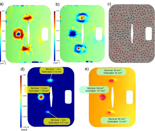
c) comparison between estimated and nominal size of defects [mm] when using all GNIF sample points d) estimating the area of defects [mm2]. ... 93 Figure 4-8: Schematic diagram of the proposed sample point filtration method. ... 95 Figure 4-9: a) distribution of the difference in maximum curvature (𝐾1) [mm-1_{] b)} distribution of the difference in minimum curvature (𝐾2) [mm-1_{] c) sample points} filtered using the curvature criterion (represented as blue spots) d) comparison between estimated and nominal size of defects [mm] when using sample points after filtering based on the curvature criterion e) estimating the area of defects [mm2]. 97 Figure 4-10: a) distribution of von Mises stress [Pa] after FENR when using GNIF sample points after filtering based on the curvature criterion b) sample points filtered using both curvature and von Mises stress criteria (represented as blue spots) c) comparison between estimated and nominal size of defects [mm] when using GNIF sample points after filtering based on both curvature and von Mises stress criteria d) estimating the area of defects [mm2]. ... 99 Figure 4-11: Interest of using the two filters successively. ... 102 Figure 4-12: a) GNIF sample points on the CAD model represented as red spots b) comparison between deformed CAD and scanned models when using all GNIF sample points [mm]. ... 103 Figure 4-13: a) distribution of the difference in maximum curvature (𝐾1) [mm-1_{] b)} distribution of the difference in minimum curvature (𝐾2) [mm-1_{] c) sample points} filtered using the curvature criterion (represented as blue spots) d) comparison between deformed CAD and scanned models when using GNIF sample points after filtering based on the curvature criterion [mm]. ... 104 Figure 4-14: a) distribution of von Mises stress [Pa] after FENR when using GNIF sample points after filtering based on the curvature criterion b) sample points filtered using curvature and von Mises stress criteria (represented as blue spots) c) comparison

(24)

between deformed CAD and scanned models when using GNIF sample points after filtering based on both curvature and von Mises stress criteria [mm]. ... 105 Figure 4-15: Synthesis of validation cases. ... 107 Figure 4-16: Side view of the CAD model for part A (in green) compared with the scanned model in a free-state (in brown) with a) bending deformation b) torsion deformation. ... 108 Figure 4-17: Part A with small (local) defects and torsion a) GNIF sample points on the CAD model represented as red spots b) comparison between estimated and nominal size of defects [mm] based on using all GNIF sample points. ... 108 Figure 4-18: Part A with small (local) defects and torsion a) distribution of the difference in maximum curvature (𝐾1) [mm-1_{] b) distribution of the difference in minimum} curvature (𝐾2) [mm-1_{] c) sample points filtered using the curvature criterion} (represented as blue spots) d) comparison between estimated and nominal size of defects [mm] when using GNIF sample points after filtering based on the curvature criterion. ... 109 Figure 4-19: Part A with small (local) defects and torsion a) distribution of von Mises stress [Pa] after FENR based on GNIF sample points after filtering using the curvature criterion b) sample points filtered using curvature and von Mises stress criteria (represented as blue spots) c) comparison between estimated and nominal size of defects [mm] when using GNIF sample points after filtering based on both curvature and von Mises stress criteria. ... 110 Figure 4-20: Part A with a big (global) defect and bending a) GNIF sample points on the CAD model represented as red spots b) comparison between estimated and nominal size of defects [mm] when using all GNIF sample points. ... 112 Figure 4-21: Part A with a big (global) defect and bending a) distribution of the difference in maximum curvature (𝐾1) [mm-1_{] b) distribution of the difference in minimum} curvature (𝐾1) [mm-1_{] c) sample points filtered using the curvature criterion}

(25)

(represented as blue spots) d) comparison between estimated and nominal size of defects [mm] when using GNIF sample points after filtering based on the curvature criterion. ... 113 Figure 4-22: Part A with a big (global) defect and bending a) distribution of von Mises stress [Pa] after FENR when using GNIF sample points after filtering based on the curvature criterion b) sample points filtered using curvature and von Mises stress criteria (represented as blue spots) c) comparison between estimated and nominal size of defects [mm] when using GNIF sample points after filtering based on both curvature and von Mises stress criteria. ... 114 Figure 4-23: Part A with a big (global) defect and torsion a) GNIF sample points on the CAD model represented as red spots b) comparison between estimated and nominal size of defects [mm] when using all GNIF sample points. ... 116 Figure 4-24: Part A with a big (global) defect and torsion a) distribution of the difference in maximum curvature (𝐾1) [mm-1_{] b) distribution of the difference in minimum} curvature (𝐾1) [mm-1_{] c) sample points filtered using the curvature criterion} (represented as blue spots) d) comparison between estimated and nominal size of defects [mm] when using GNIF sample points after filtering based on the curvature criterion. ... 117 Figure 4-25: Part A with a big (global) defect and torsion a) distribution of von Mises stress [Pa] after FENR based on GNIF sample points after filtering using the curvature criterion b) sample points filtered using curvature and von Mises stress criteria (represented as blue spots) c) comparison between estimated and nominal size of defects [mm] when using GNIF sample points after filtering based on both curvature and von Mises stress criteria. ... 118 Figure 4-26: CAD model along with GD&T specification for part B (dimensions are in mm). ... 120 Figure 4-27: GNIF corresponding sample points (in black) on the CAD and scanned models of part B. ... 121

(26)

Figure 4-28: Side view of CAD model for part B (in green) compared with the scanned model (in brown) a) with bending deformation b) with torsion deformation. ... 121 Figure 4-29: Part B with small (local) defects and bending a) and f) initial and filtered sample points c) and d) distribution of the difference in principle curvatures [mm-1] e) distribution of von Mises stress [Pa] after the second FENR. b) and g) comparison between estimated and nominal size of defects [mm] based on initial and filtered sample points. ... 122 Figure 4-30: Part B with small (local) defects and torsion a) and f) initial and filtered sample points c) and d) distribution of the difference in principle curvatures [mm-1] e) distribution of von Mises stress [Pa] after the second FENR. b) and g) comparison between estimated and nominal size of defects [mm] based on initial and filtered sample points. ... 126 Figure 4-31: Part B with a big (global) defect and bending a) and f) initial and filtered sample points c) and d) distribution of the difference in principle curvatures [mm-1] e) distribution of von Mises stress [Pa] after the second FENR. b) and g) comparison between estimated and nominal size of defects [mm] based on initial and filtered sample points. ... 129 Figure 4-32: Part B with a big (global) defect and torsion a) and f) initial and filtered sample points c) and d) distribution of the difference in principle curvatures [mm-1] e) distribution of von Mises stress [Pa] after the second FENR. b) and g) comparison between estimated and nominal size of defects [mm] based on initial and filtered sample points. ... 131 Figure 5-1: A regular aerospace panel, a) in free-state, b) constrained by fixing jigs on the inspection fixture [2]. ... 140 Figure 5-2: 3D view of the CAD model of a non-rigid aluminum panel. ... 144 Figure 5-3: GNIF corresponding sample points (in black) are located in the center of colorful zones on the CAD and scanned models. ... 145

(27)

Figure 5-4: a) all GNIF sample points inserted into the CAD mesh based on classical Delaunay method (red spots) b) automatic sample point filtration based on curvature and von Mises stress criteria and criteria (blue spots). ... 146 Figure 5-5: Definition of maximum amplitude 𝐷𝑖𝑚𝑎𝑥 and area of a defect𝐴𝑖. ... 147 Figure 5-6: a) the scanned part with the nominal dimensions of defects b) estimated and nominal maximum amplitude (𝐷𝑖𝑚𝑎𝑥) of defects [mm] c) estimated and nominal area (𝐴𝑖 shown as red zones) of defects [mm2_{]. ... 147} Figure 5-7: Flowchart of our automatic fixtureless CAI method. ... 148 Figure 5-8: defects are identified as red zones based on the tolerance value (0.4 mm) a) for nominal defects b) for estimated defects. ... 153 Figure 5-9: CDF for nominal and estimated defects for Bump #1 and Bump #2. ... 154 Figure 5-10: Estimation of the distance distribution of a defect a) nominal defect, b) for an accurate inspection c) for an overestimated defect d) for a badly estimated defect. ... 155 Figure 5-11: a) a noise-free scan mesh b), c), d) scan meshes with synthetic noise with Gaussian distribution with zero mean value and standard deviation equal to b) 0.01mm c) 0.02mm d) 0.03mm. ... 156 Figure 5-12: Synthesis of validation cases with small free-state deformation... 158 Figure 5-13: CAD model along with GD&T specification for part A (dimensions are in mm). ... 160 Figure 5-14: a) nominal defect distance distribution for part A with small (local) defects, comparison between the CAD and scanned model of part A with small (local) defects and bending deformation as a distance distribution for b) noise-free scan mesh c) noisy scan mesh with σ=0.01 mm d) noisy scan mesh with σ=0.02 mm e) noisy scan mesh with σ=0.03 mm... 161

(28)

Figure 5-15: a) the scanned part with the nominal dimensions of big (global) defect b) nominal defect distance distribution for part A with a big (global) defect, comparison between the CAD and scanned model of part A with a big (global) defect and bending deformation as a distance distribution for c) noise-free scan mesh d) noisy scan mesh with σ=0.01 mm e) noisy scan mesh with σ=0.02 mm f) noisy scan mesh with σ=0.03 mm. ... 165 Figure 5-16: CAD model along with GD&T specification for part B (dimensions are in mm). ... 168 Figure 5-17: Side views of the CAD model for part B (in green) compared with scan data in a free-state (in brown) with a) bending deformation b) torsion deformation. .. 168 Figure 5-18: a) nominal defect distance distribution for part B with small (local) defects, comparison between the CAD and scanned model with small (local) defects and bending deformation as a distance distribution for b) noise-free scan mesh c) noisy scan mesh with σ=0.01 mm d) noisy scan mesh with σ=0.02 mm e) noisy scan mesh with σ=0.03 mm. ... 170 Figure 5-19: a) nominal defect distance distribution for part B with small (local) defects, comparison between the CAD and scanned model with small (local) defects and torsion deformation as a distance distribution for b) noise-free scan mesh c) noisy scan mesh with σ=0.01 mm d) noisy scan mesh with σ=0.02 mm e) noisy scan mesh with σ=0.03 mm. ... 173 Figure 5-20: a) nominal defect distance distribution for part B with a big (global) defect, comparison between the CAD and scanned model with a big (global) defect and bending deformation as a distance distribution for b) noise-free scan mesh c) noisy scan mesh with σ=0.01 mm d) noisy scan mesh with σ=0.02 mm e) noisy scan mesh with σ=0.03 mm. ... 176 Figure 5-21: a) nominal defect distance distribution for part B with a big (global) defect, comparison between the CAD and scanned model with a big (global) defect and torsion deformation as a distance distribution for b) noise-free scan mesh c) noisy

(29)

scan mesh with σ=0.01 mm d) noisy scan mesh with σ=0.02 mm e) noisy scan mesh with σ=0.03 mm. ... 178 Figure 5-22: Error intervals for part B with respect to the increase of noise amplitude.

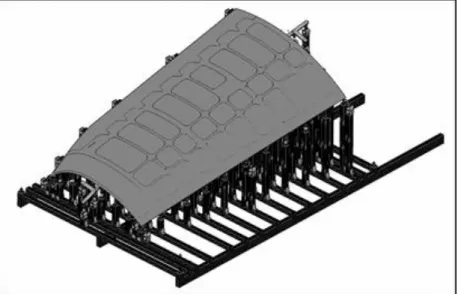
... 181 Figure 5-23: 3D views of CAD model (in green) compared with scan data in a free-state (in brown) for part A with a) small bending deformation b) large bending deformation. ... 182 Figure 5-24: a) nominal defect distance distribution for part A with small (local) defects, comparison between the CAD and scanned model of part A with small (local) defects and large bending deformation as a distance distribution for b) noise-free scan mesh c) noisy scan mesh with σ=0.01 mm d) noisy scan mesh with σ=0.02 mm e) noisy scan mesh with σ=0.03 mm. ... 183 Figure 5-25: a) nominal defect distance distribution for part A with a big (global) defect, comparison between the CAD and scanned model of part A with a big (global) defect and large bending deformation as a distance distribution for b) noise-free scan mesh c) noisy scan mesh with σ=0.01 mm d) noisy scan mesh with σ=0.02 mm e) noisy scan mesh with σ=0.03 mm. ... 186 Figure 5-26: Absolute error (in %) in the estimation of defects for part A for small versus large deformation. ... 188 Figure 6-1: An ordinary aerospace panel a) in free-state, b) constrained on supports of the inspection fixture [1]. ... 201 Figure 6-2: An aerospace panel under permissible restrained loads (the weight of black sandbags applied on the surface of part) achieves the functional shape on physical fixture [1]. ... 202 Figure 6-3: Schematic flowchart of the proposed assembly assessing method. ... 211 Figure 6-4: Analysis of geometrical offset based on GD&T specification. ... 218

(30)

Figure 6-5: Schematic misalignment of assembly mounting hole on predicted shape of scan model with respect to the CAD model. ... 219 Figure 6-6: Flowchart algorithm of proposed VMASI method. ... 220 Figure 6-7: Synthesis of validation cases with different types of defects. ... 222 Figure 6-8: GD&T specification for part A (dimensions are in mm). ... 224 Figure 6-9: a) Displacement distribution [mm] of deviated scan model generated by decreasing 1 deg. of forming angle; b) The partitioned scan model and predicted assembly pressure... 227 Figure 6-10: a) Displacement distribution [mm] of deviated scan model generated by decreasing 3 deg. of forming angle; b) The partitioned scan model and predicted assembly pressure... 229 Figure 6-11: a) Displacement distribution [mm] of deviated scan model generated by decreasing 5 deg. of forming angle; b) The partitioned scan model and predicted assembly pressure... 230 Figure 6-12: a) Displacement distribution [mm] of slightly deviated scan mesh simulating a plastic defect; b) The partitioned scan model and predicted assembly pressure. ... 232 Figure 6-13: a) displacement distribution [mm] of deviated scan mesh simulating a plastic defect; b) the partitioned scan model and predicted assembly pressure. ... 233 Figure 6-14: a) The manufactured part mounted on inspection fixtures where a real point cloud of scan mesh can be acquired, in our proposed method only 9 fixation features are kept as datums; b) GD&T specification for part B (dimensions are in mm). . 236 Figure 6-15: a) Displacement distribution [mm] of deviated scan mesh simulating a small plastic defect; b) The partitioned scan model and predicted assembly pressure. . 238

(31)

Figure 6-16: a) Displacement distribution [mm] of deviated scan mesh simulating an intermediate plastic defect; b) the partitioned scan model and predicted assembly pressure. ... 241 Figure 6-17: a) Displacement distribution [mm] of deviated scan mesh simulating a large plastic defect; b) the partitioned scan model and predicted assembly pressure. ... 244 Figure 7-1: 3D views of CAD model (in green) compared with scan model in a free-state (in brown) simulated based on large displacement formulation. ... 255 Figure 7-2: Remained sample points (as red spots) after applying filtering registration points method using a) nonlinear FENR for noise-free scan mesh b) linear FENR for noise-free scan mesh c) nonlinear FENR for noisy scan mesh with σ=0.01 mm d) linear FENR for noisy scan mesh with σ=0.01 mm. ... 256 Figure 7-3: Distribution of von Mises stress [Pa] when using GNIF sample points after a) nonlinear FENR for noise-free scan mesh b) linear FENR for noise-free scan mesh c) nonlinear FENR for noisy scan mesh with σ=0.01 mm d) linear FENR for noisy scan mesh with σ=0.01 mm. ... 257 Figure 7-4: a) nominal defect distance distribution, comparison between the deformed CAD and scan models as a distance distribution using b) nonlinear FENR for noise-free scan mesh c) linear FENR for noise-noise-free scan mesh d) nonlinear FENR for noisy scan mesh with σ=0.01 mm e) linear FENR for noisy scan mesh with σ=0.01 mm. ... 259 Figure 8-1: A synthesis of contributions in the thesis. ... 265

(32)

LIST OF SYMBOLS

𝐷_𝑖𝑚𝑎𝑥 Maximum amplitude of a defect i 𝐴_𝑖 Area of a defect i

𝑁𝑑𝑒𝑓𝑒𝑐𝑡 Number of identified defects

𝐻₀ Null hypothesis 𝐻_𝐴 Alternative hypothesis 𝐷𝑑𝑎 Nominal defect 𝐷𝑑_𝑒 Estimated defect σ Standard deviations μ Mean value

𝒮𝐶𝐴𝐷 Set of nodes on CAD mesh

𝒟𝐶𝐴𝐷 Set of nodes on inspection datums of CAD mesh

ℐ𝐶𝐴𝐷 Set of nodes on inspecting mounting holes of CAD mesh 𝒮𝑆𝐶𝑁 _{Set of nodes on scan mesh}

𝒟𝑆𝐶𝑁 _{Set of nodes on inspection datums of scan mesh} 𝒮 Set of nodes on scan mesh after pre-registration

𝒟 Set of nodes on inspection datums of scan mesh after pre-registration ℐ Set of nodes on inspecting mounting holes of scan mesh after

pre-registration

𝓣 List of partitioned zones on scan mesh after pre-registration ∆ Distance between mounting holes on scan and CAD meshes

(33)

LIST OF ABBREVIATIONS

CAD Computer-Aided Design CAI Computer-Aided Inspection

GD&T Geometric Dimensioning and Tolerancing GNIF Generalized Numerical Inspection Fixture FEA Finite Element Analysis

FENR Finite Element Non-rigid Registration K-S test Kolmogorov–Smirnov test

VMASI Virtual Mounting Assembly-State Inspection RPO Restraining Pressures Optimization

ICP Iterative Closest Point

IDI Iterative Displacement Inspection RBFs Radial Basis Functions

GMDS Generalized Multidimensional Scaling FMA Fast Marching Algorithm

RNIF Robust generalized Numerical Inspection Fixture V&V Verification and Validation

(34)

PREFACE

This research work is part of a collaborative research program on the metrology of non-rigid (flexible) parts. The project is defined in the framework of the Consortium de recherche et d'innovation en aérospatiale au Québec (CRIAQ), which is referred as CRIAQ MANU501. The industrial partners of this project are Bombardier Aerospaceand CREAFORMcompanies. Three universities that are engaged in this project include École de Technologie Supérieure (ÉTS), Université du Québec à Trois-Rivières (UQTR) and Université de Sherbrooke.

This thesis is composed as a paper-based thesis and consists of eight chapters. In Chapter 1, an introduction concerning the compliant behavior of non-rigid (flexible) parts, conventional inspection methods and Computer-Aided Inspection (CAI) methods is presented. In Chapter 2, a comprehensive literature review regarding the different types of scanning tools, and developed fixtureless CAI methods along with their advantages and drawbacks are presented. The general planning comprising the statement of problems and objectives of this thesis are explained in Chapter 3. Chapter 4, Chapter 5 and Chapter 6 are assigned to the articles submitted to scientific journals. These articles describe the improvements and developments of original methods for automatic inspection of non-rigid parts and robustness validation of the methods. This thesis is ended with a general discussion, various perspectives, and conclusions that are presented in Chapter 7 and Chapter 8.

(35)

CHAPTER 1 INTRODUCTION

Improvements in the metal forming industry lead to manufacturing of complex parts that are commonly used in different industrial sectors among which aerospace and automobile. These complex parts may include many details, features and complex freeform shapes. The quality, efficiency, and functionality of these parts are controlled by Geometric Dimensioning and Tolerancing (GD&T) approaches. Manufacturing companies attempt to maintain in the competitive markets by producing high-quality parts. The quality control (QC) process, consisting of geometrical and dimensional controls, ensures the functionality of products. However, conventional inspection methods are costly, time-consuming and require manual intervention. Despite the progress in manufacturing methods for reducing the lead time of production, the quality control is still a time-consuming challenge. For example, some inspection setup for non-rigid parts in Bombardier Aerospace company demands 60 to 75 hours of operation (Radvar-Esfahlan and Tahan 2014). Therefore, the recent concern of manufacturing companies is to perform an accurate dimensional inspection in a short time. Thin walled sheet metals, which are commonly used in industrial sectors among which the aerospace and automotive, present a more serious challenge for geometrical and dimensional inspection in a quality control process. These sheet metals have a small thickness compared to the other dimensions, which gives them flexible behavior during inspection. The flexibility of these non-rigid parts is referred to as compliant behavior in tolerancing contexts. These non-rigid parts may deform during a free-state inspection process, which is the main issue in GD&T. The compliance in a free-state can take place due to the weight of the part, residual stress (release of internal stress resulting from manufacturing) remaining in the part during the manufacturing process or any geometrical deviation. Metrology standards such as ASME Y14.5 and ISO-1101-GPS require performing the inspection of parts in free-state unless otherwise specified. The exceptions to this rule, as mentioned in standards ASME Y14.5 (2009) and ISO-10579-GPS, are for non-rigid parts. In fact, free-state refers to a situation that a part is not constrained and is not submitted to

(36)

any load except its weight. A non-rigid aerospace panel in a free-state, as shown in Figure 1-1-a, is deformed due to the weight on an inspection table. Conventional inspection methods use over constrained fixtures for non-rigid parts. In some cases, the functional shape of a non-rigid part can be retrieved by using these fixtures and by restraining the part under permissible loads during the dimensional inspection process. Therefore, even though the shape variation of parts exceeds the allocated dimensioning tolerances, these non-rigid parts can still be assembled. Improvements in digital data acquisition devices such as 3D optic and laser scanners (Bi and Wang 2010) along with the computational calculation developments lead to Computer-Aided Inspection (CAI) methods. The 3D data acquisition tools obtain a set of points, namely point clouds, from the surface of parts during the inspection process. The scan mesh is then generated from the raw scanning data (point clouds), which is processed by mesh smoothing methods as presented by (Karbacher and Haeusler 1998). This scan mesh intends to accurately represent the geometrical shape of the part with the least required data volume (mesh size). CAI methods apply tolerancing methods along with computational meshing tools to implement an automatic and time-saving inspection. In fact, CAI methods make the comparison between the Computer-Aided Design (CAD) model and the scan range data in a common coordinate system to evaluate the geometrical deviations (defects) of the part. Since the CAD model is in the Design Coordinate System (DCS) and the scan data in the Measurement Coordinate System (MCS), registration methods developed in CAI context are required to align the CAD and scan models in a common coordinate system. Considering the flexible deformation of parts in a free-state, the comparison between CAD and scan models cannot estimate defects size on scan model. To resolve this problem, CAI methods for non-rigid parts are used to distinguish between the defects (such as geometrical deviations and distortions with respect to CAD model) and the flexible deformation (due to the compliance) of non-rigid parts. As already mentioned, conventional dimensioning and inspection methods for non-rigid parts sets up over-constrained inspection fixtures to compensate for the flexible deformation of these parts and to ensure that the measurement setup properly represents the assembly functionality

(37)

of the part (Ascione and Polini 2010). These fixtures also retrieve the functional shape of the part and align it with the reference frame during the measuring process. Figure 1-1-b illustrates an example of such an inspection fixture for the part. The same part is demonstrated in Figure 1-1-a at a free-state.

Figure 1-1: An ordinary aerospace panel, a) in free-state, b) constrained on supports of the inspection fixture (Abenhaim, Desrochers et al. 2015)

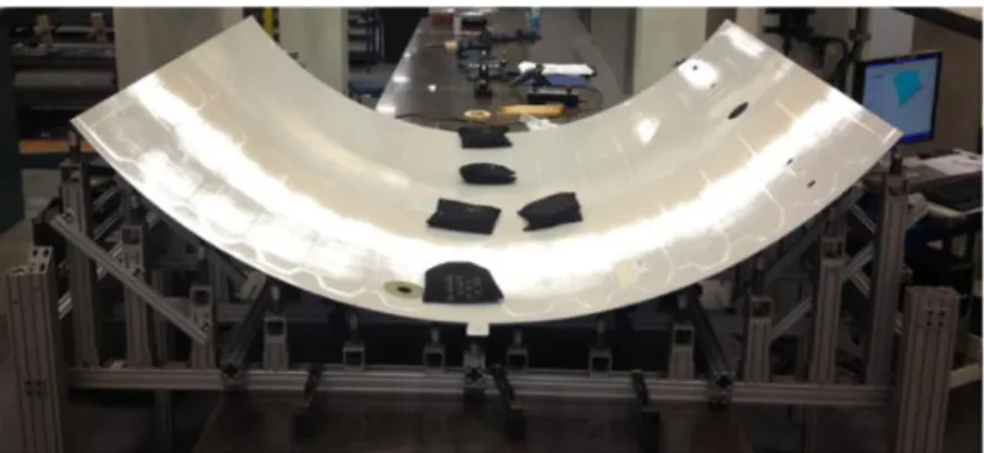
Moreover, dimensional inspection of non-rigid parts is generally accomplished in restrained conditions such as assembly loads, supports and clamps (Abenhaim, Desrochers et al. 2012). As shown in Figure 1-2, a practical inspection technique applies weights (e.g. sandbags) on the surface of a deviated non-rigid part to retrieve its functional shape constrained on a physical fixture. These weights are permissible assembly loads that are commonly presented as a note in design drawings authorizing their application during the inspection process. The limits for permissible loads are defined to prevent permanent deviations (plastic deformation) during the inspection and eventually assembly process. In drawings, a note such as “A load of X N/m2 can be used to achieve tolerance” is indicated next to the associated geometrical requirements specifying the permissible loads and the associated fixture. Therefore, a non-rigid part can be restrained by assembly loads that are limited to the given permissible values during the inspection. These restraining loads are usually used for large non-rigid parts such as aerospace panels for which the functional shape of parts can be retrieved by imposing constraints during assembly.

(38)

Figure 1-2: An aerospace panel restrained under known loads by using weights (the black sandbags) on its surface (Abenhaim, Desrochers et al. 2015).

Serious drawbacks of using physical inspection fixtures lead to developing fixtureless CAI methods to eliminate the need for costly and complex physical fixtures. These methods apply computational techniques to distinguish between defects and flexible deformation. This intends to virtually compensate for the flexible deformation of non-rigid parts in a free-state. The primary step for inspection of non-non-rigid parts is a pre-registration using rigid pre-registration methods. Rigid pre-registration brings the CAD and scan models closer in a common coordinate system using a transformation matrix. Among different rigid registration methods (Li and Gu 2004, Savio, De Chiffre et al. 2007), the Iterative Closest Point (ICP) algorithm (Besl and Mckay 1992) is widely applied in different domains. ICP algorithm provides a robust and efficient registration method for rigid parts. Applying pre-registration the CAD and scan models are aligned and brought closer without deforming the models. In fact, rigid registration does not take into consideration the flexible deformation of non-rigid parts. However, fixtureless CAI methods presented in section 2.4.2 enable the inspection by virtually compensating for the flexible deformation of scan models in a free-state. This allows the estimation of defects on the manufactured parts with respect to the nominal CAD models. In general, these fixtureless non-rigid registration methods search for correspondence between the CAD and scan models to deform the CAD or scan model towards the other one. This is performed by using FEA or gradually iterative displacements. Non-rigid registration methods based on deforming the scan mesh towards the CAD model are presented in

(39)

section 2.4.2.1, and non-rigid inspection methods based on deforming the CAD model towards the scan mesh are introduced in section 2.4.2.2. However, these non-rigid registration methods are not fully automated. An automatic fixtureless CAI for non-rigid parts that is capable of identifying and estimating both small (local) and big (global) defects is presented in Chapter 4. This method applies corresponding sample points to determine displacement boundary conditions (BCs) for a Finite Element Non-Rigid Registration (FENR). Distinguishing between the flexible deformation and defects, the sample points close and on defect areas are filtered out based on curvature and von Mises stress criteria. This leads to an accurate and automatic fixtureless CAI for non-rigid parts. Once a CAI method is developed, the robustness and performance of the method should be verified and validated with respect to actual measurements. To this end, a quantitative validation metric applied in a Verification and Validation (V&V) method is required. In Chapter 5, a new validation metric for fixtureless CAI methods is presented which analyses the robustness of CAI method with respect to scanning noise. This validation metric applies statistical hypothesis testing to validate whether the distance distribution of nominal and estimated defects are sufficiently similar.

Most of these developed fixtureless inspection methods do not take into consideration restraining loads. These loads are permitted to be used for placing deviated non-rigid parts into assembly state and are commonly mandated during inspection process especially for large parts such as aerospace panels. It should be considered that defects on non-rigid parts can generally occur during manufacturing and handling processes. In Chapter 6, a non-rigid registration method is proposed that aims to evaluate the feasibility of putting a deviated part in assembly-state. In fact, defects such as warpage, shrinkage or any type of plastic deformation on non-rigid parts result in misalignment at the assembly. However, excessive geometrical variations with respect to the assembly tolerance would be absorbed by the compliance of non-rigid parts. The developed Virtual Mounting Assembly-State Inspection (VMASI) method applies a new registration to virtually retrieve the functional shape of deviated parts under permissible assembly loads. The inspection is accomplished by verifying fixation features (e.g. mounting holes) on the

(40)

predicted shape of scan mesh in assembly-state with respect to the allocated assembly tolerances. The feasibility of mounting a geometrically deviated non-rigid part in assembly-state is approved when all mounting holes on the predicted shape of scan mesh are in the tolerance range.

1.1 Structure of the thesis

This thesis is composed in the form of article-based thesis wherein three articles are presented and logically connected to each other. The methodologies, results, and discussions are presented in detail inside the articles. These articles have been submitted for publication in scientific international journals with reviewing committees, which are recognized in their respective fields (advanced manufacturing for the first article, ASME V&V for the second article and Computer-Aided Design for the third article). As presented in Figure 1-3, at the time of writing this thesis, the first article is already published, the second and third articles are submitted and they are currently under review. This thesis is enclosed in 8 chapters. A comprehensive literature review consisting of the non-rigid parts specifications, scanning tools, rigid and non-rigid registration methods for fixtureless inspection of non-rigid parts is presented in Chapter 2. In Chapter 3, the general planning of the thesis is described which consists of the statement of the problem, objectives, and hypothesis of this project. This is followed by three articles in Chapter 4, Chapter 5 and Chapter 6 respectively. A general discussion on the methodology and results of developed CAI methods and validation metric is presented in Chapter 7. Finally in Chapter 8, major contributions, perspectives for future works and conclusions of the developed methods in this thesis are presented.

(41)

(42)

CHAPTER 2 LITERATURE REVIEW

2.1 Introduction

In this chapter, a comprehensive literature review concerning the compliance of non-rigid parts along with the developed inspection methods is presented. Flexible deformation and dimensional variation of non-rigid parts in a free-state, due to the compliant behavior, conventionally require inspection fixtures to recover their functional shape. These flexible deformations are due to gravity loads, residual stress, and/or assembly force. Meanwhile, dedicated fixtures such as conformation jigs should be provided in two sets for the supplier and the client for the sake of independent and repeatable inspection. To resolve these obstacles, Computer-Aided Inspection (CAI) methods are developed in which the fast and accurate scanning devices along with computational calculations are exploited. The fixtureless and automated CAI methods, which eliminate the need for complex fixtures are time and money savers for industrial sectors. The robustness, efficiency, and reliability of these numerical methods can also be evaluated quantitatively. This chapter discusses background information in regards to the compliant behavior of non-rigid parts. The classification associated with the flexibility of the parts is presented in section 2.2. Then, different 3D digitization tools, which include scanners are described in section 2.3. Different inspection methods including rigid and non-rigid registration algorithms are explained in section 2.4. A review on different Verification and Validation (V&V) methods and their application in several disciplines of computational mechanical engineering are introduced in section 2.5. At the end of this chapter, section 2.6, a summary of the state of the art is given.

2.2 The compliance of non-rigid parts

The definition of compliant behavior (compliance) for non-rigid parts is related to material and geometrical flexibility of parts. In fact, the higher compliance value of parts implies the higher flexibility of these parts. Therefore, the flexible deformation of

(43)

non-rigid parts in a free-state is due to the compliant behavior of these parts. Considering the notation of finite element analysis, [𝐾]{𝑢} = {𝑓}, the compliance (𝐶) is defined in Equation 2-1.

𝐶 = {𝑢}𝑡_{𝑓} _2-1

Where {𝑓} is the force vector, [𝐾] is the global stiffness matrix and {𝑢} is the displacement vector. The flexibility is defined as the inverse of stiffness ([𝐾]−1) accordingly.

A classification for the compliance of parts is represented in (Abenhaim, Desrochers et al. 2012). The proposed force value in this classification is the permissible force, which is commonly applied during manual assembly lines and inspection techniques in the aerospace industry. The classification for compliance of parts, as depicted in Figure 2-1 and Table 2-1, categories parts in three behavior zones (zone A, B, and C). It describes that parts in zone A are considered practically as rigid parts. The induced displacement of a rigid part due to a reasonable assembly force (around 40 N) is insignificant (less than 5% of the assigned tolerance). The parts categorized in zone B are considered as non-rigid parts where the induced displacement is over 10% of the assigned tolerances. These non-rigid parts, such as thin-walled sheet metals, are commonly used in different industrial sectors such as automobile and aerospace industries. As defined in ISO-GPS standard, the flexible deformation of non-rigid parts in a free-state is beyond the dimensional and/or geometrical tolerances. This standard determines free-state as a condition that parts are not subjected to any constraining load. In fact, these parts in a free-state are submitted only to their own weight during inspection process. The parts associated with the compliant behavior in zone C enclose extremely non-rigid parts such as seals and tissues for which the part shape is extremely dependent on the part orientation and weight.

(44)

Figure 2-1: Classification of the compliant behavior of parts (Abenhaim, Desrochers et al. 2012).

Table 2-1: The classification for compliant behavior of parts concerning the induced displacement under applied force (Abenhaim, Desrochers et al. 2012).

Zones Displacement under permissible assembly

force during inspection (~40 N) Compliant behavior of parts A < 5-10% of the assigned tolerance Rigid

B > 10% of the assigned tolerance Non-rigid (Flexible) C >>10% of the assigned tolerance Extremely Non-rigid

2.3 Measurement and 3D data acquisition methods

The traditional measuring methods apply measuring techniques that are operated by using special metrology devices such as inspection fixtures. These time-consuming techniques require skillful operators. However, developments in 3-D scanning technology allow creating a digital scan model from a physical object. Concerning the developed measuring systems (Savio, De Chiffre et al. 2007) and specifically laser scanners (Martínez, Cuesta et al. 2010), these measuring devices (scanners) can be categorized as contact and non-contact scanners.