Direct and semi-direct aerosol effects on
the southern African regional climate
during the austral winter season
Fiona Tummon
Thesis Presented for the Degree of
DOCTOR OF PHILOSOPHY
Acknowledgements
There are a great many people to thank for all the help, support, patience and encouragement that I’ve needed during the past three years. Firstly, I am deeply indebted to Fabien Solmon for his thorough and insightful supervision, for always being ready to answer my innumerable questions, no matter how mundane and for keeping a sense of humour throughout it all. I am also extremely grateful to Mark Tadross and Bruce Hewitson for their guidance, endless stream of interesting ideas and their invaluable criticism along the way. The enthusiasm of all three of my supervisors and their passion for their work is contagious and the immense depth of their knowledge has been of great inspiration.
Secondly, this thesis would never have been possible without the financial support of a CNRS bourse BDI-PED and, for the final months, the IDAF project. A big thank you is also due to CSAG and the LA for financing my trips between Cape Town and Toulouse (and especially for allowing me to experience an endless summer for almost two years).
Being split between two continents has been far from easy, but everyone from CSAG and the LA have always welcoming, willing to help and made the past three years a terrific experience. Special thanks to Cathy Liousse for her commitment, enthusiasm and all the informative discussions along the way, as well as to Robert Rosset for his continuous supply of useful articles. A very big thank you is also due to all the IT staff at the CHPC and CSAG in Cape Town, especially Jeremy Main and Chris Jack, for helping me through the somewhat painful process of installing RegCM. Also, to the IT staff at the LA in Toulouse, an enormous thank you – for always being ready to come to the rescue with a smile on their faces and taking the time to fix whatever problem there was, no matter how small.
Finally, for their continuous support, encouragement and always believing in me even when I didn’t, I thank my fabulous family (mom, dad and Oisin) and my friends, old and new, who’ve been there for the journey: Susanna, Steffi, Daniel, Eric-Michel, Héloise, Rebecca, Justin, Michaela, Erwan, Laurie, Vivija and Gosia, amongst the many others. The past three years would quite simply not have been the same had it not been for the kindness, care, willingness to listen and the weekend adventures shared with these people. Merci vraiment beaucoup!!
Abstract
The regional climate model RegCM3 is used to investigate the direct and semi-direct aerosol effects on the southern African climate during the austral winter season (June-September). The sensitivity of simulated aerosol-climate effects to different biomass burning inventories, boundary conditions and sea surface temperature (SST) feedbacks is tested to assess the range of uncertainty associated with these parameters. Sensitivity to both boundary forcing and SST feedbacks appears to be negligible, while the aerosol radiative forcing (RF) is found to vary approximately linearly in response to aerosol emissions (varying by up to a factor of two in response to the factor of two difference between emissions inventories). In all cases the surface RF is negative, while the top-to-atmosphere RF is negative over most of the domain but positive over high-albedo savannah regions where aerosol loading is concentrated. Although the magnitude of simulated RF varies depending on the biomass burning emissions inventory used, all simulations show similar aerosol-climate impacts. Surface temperature decreases over most of the subcontinent, a signal which acts to reduce model bias over the western half of the region. The absorbing nature of the simulated aerosol burden results in heating at altitude, which, in combination with the surface cooling, serves to increase stability in the lower atmosphere over most of the subcontinent. In the middle troposphere, however, this warming induces an elevated heat-pump effect in the equatorial regions between approximately 8°N and 5°S. This enhances convection, precipitation as well as soil moisture and effectively acts to spin-up the hydrological cycle in the tropics. An investigation of the interannual variability of seasonal average aerosol impacts shows that significant difference in variability is apparent only in the main biomass burning regions, where aerosol loading is highest. The seasonal average precipitation changes varies more from year to year than aerosol-induced surface temperature changes, likely as a result of the greater variability associated with convective processes controlling precipitation in the regions affected. In contrast, despite there being significant differences between synoptic conditions, there is little synoptic-scale variability of aerosol-climate impacts. This suggests that, at least on the synoptic-scale, the atmospheric aerosol loading is more sensitive to the magnitude of emissions than any other control.
Résumé
Le modèle climatique régional RegCM3 est utilisépour examiner les effets direct et semi-direct des aérosols sur le climat du sud de l'Afrique pendant l'hiver austral (juin-septembre). La sensibilité des effets simulés aux différents inventaires d'émissions de combustion de biomasse et aux différentes conditions aux limites est evaluer, afin d'estimer l'incertitude associée à ces paramètres. La sensibilité aux conditions aux limites derivées de réanalyses est modeste, mais le forçage radiatif des aérosols varie linéairement en réponse au différents inventaires testées jusqu'à un facteur deux. Le forçage radiatif est toujours négatif, alors que le forçage radiatif au sommet de l'atmosphère est negatif sur la plupart du domaine sauf au-dessus les régions de savane ou le contenu atmosphérique d'aérosols est élevée. Même si la magnitude du forçage radiatif varie, les simulations pour la période présente montrent des impacts climatiques comparables. La température de surface diminue sur la plupart de la région, ce signale qui réduit le biais du modèle sur l'ouest du sous-continent. L'échauffement en altitude est lié à la charge d'aérosols absorbants et cela, en combinaison avec la réduction de température en surface, mène à la stabilisation de la basse atmosphère. Toutefois, dans la moyenne troposphère de la zone équatoriale (entre 8°N et 5°S) cet échauffement à pour résultat un effet de 'pompe à chaleur en altitude'. Cet effet augmente la convection, les précipitations et l'humidité du sol, en accélérant le cycle hydrologique dans cette région. Une étude de la variabilité interannuelle des effets climatiques des aérosols montre que les changements des précipitations en moyenne saisonnière sont plus variables d'un an à l'autre que les changements de température de surface. Par contre, malgré des différences significatives entre les conditions synoptiques, la variabilité synoptique des impacts climatiques des aérosols est faible.
Abbreviations
AAO – Antarctic OscillationAEJ-N – African Easterly Jet - Northern branch AEJ-S – African Easterly Jet - Southern branch AERONET – Aerosol Robotic Network
AMMA – African Monsoon Multidisciplinary Analyses AOD – Aerosol Optical Depth
BATS – Biosphere-Atmosphere Transfer Scheme BC – Black Carbon
CCM – Community Climate Model CCN – Cloud Condensation Nuclei CLWP – Cloud Liquid Water Path
CMAP – CPC Merged Analysis of Precipitation CPC – Climate Prediction Centre
CRU – Climate Research Unit (of the University of East Anglia)
DEBITS – Deposition of Biogeochemically Important Species (umbrella project of IGAC) DJF – December/January/February
ECMWF – European Centre for Medium-range Weather Forecasting ENSO – El Niño Southern Oscillation
ERA40 – ECMWF 40-year Reanalysis GCM – Global Climate Model
GFED – Global Fire Emissions Database GLCC – Global Land Cover Characterisation GPCP – Global Precipitation Climatology Project GPH – Geopotential Height
ICTP – International Centre for Theoretical Physics IDAF – IGAC DEBITS Africa
IGAC – International Global Atmospheric Chemistry IN – Ice Nuclei
IPCC – International Panel for Climate Change ITCZ – Inter-Tropical Convergence Zone JJA – June/July/August
JJAS – June/July/August/September LW – Longwave
MAM – March/April/May MBL – Marine Boundary Layer
MISR – Multi-angle Imaging Spectro-Radiometer MIT – Massachusetts Institute of Technology MM4 – Mesoscale Model version 4
MM5 – Mesoscale Model version 5
MODIS – Moderate Resolution Imaging Spectrometer NAO – North Atlantic Oscillation
NCAR – National Centre for Atmospheric Research
NCEP-II – National Centre for Environmental Prediction reanalysis product version 2 NDVI – Normalised Difference Vegetation Index
NOAA – National Ocean Atmosphere Administration OC – Organic Carbon
PBL – Planetary Boundary Layer RCM – Regional Climate Model RegCM – Regional Climate Model RF – Radiative Forcing
RH – Relative Humidity
RMSD – Root-Mean-Square Difference SON – September/October/November SSA – Single Scattering Albedo SST – Sea Surface Temperature SW – Shortwave
TOA – Top Of Atmosphere
TOMS – Total Ozone Monitoring System TRMM – Tropical Rainfall Monitoring Mission USGS – United States Geological Surveys ZAB – Zaire Air Boundary
Contents
Acknowledgements ……….. 1
Abstract ……… 3
Résumé ……… 4
Abbreviations ………..……… 5
Chapter 1: General Introduction – Why southern Africa? Why Aerosols?
1.1 Motivation from a global perspective ……….. 131.2 Motivation at the regional level ………... 15
1.3 Why regional climate modelling? ………. 17
1.4 Goals and aims of this study ……… 19
Chapter 2: Background and Introduction
2.1 Southern Africa: a regional description ………. 222.1.1 Regional climate and mean circulation patterns ……… 22
2.1.2 Absolutely stable layers ……….. 26
2.1.3 Recirculation over southern Africa ……… 28
2.1.4 Aerosol plumes exiting the subcontinent ………. 29
2.1.5 Southern African climate variability ……… 31
2.1.6 Observed temperature and precipitation trends ……….. 33
2.1.7 Future climate projections ………... 34
2.2 Atmospheric aerosol ……….. 35
2.2.1 Aerosol formation, particle growth and size distribution ………. 36
2.2.2 Aerosol sources ………. 37 2.2.2.1 Industrial aerosol ………. 38 2.2.2.2 Carbonaceous aerosol ……….. 39 2.2.2.2.1 Black carbon ……….. 40 2.2.2.2.2 Organic carbon ……….. 41 2.2.2.3 Biomass burning ………. 41
2.2.2.4 Mineral dust aerosol ……… 45
2.2.2.5 Marine aerosol ………. 48
2.2.3 Aerosol deposition ……… 48
2.2.3.1 Dry deposition ………. 48
2.2.3.2 Wet deposition ………. 49
2.2.4 Aerosol optical properties ……… 50
2.2.4.1 Aerosol optical depth ……….. 50
2.2.4.3 Single scattering albedo ………. 51
2.2.5 Aerosol-radiation-climate interactions ……… 51
2.2.5.1 The direct aerosol effect ………. 53
2.2.5.2 The semi-direct aerosol effect ..………. 54
2.2.5.3 The indirect aerosol effects ……… 55
2.2.6 Other aerosol impacts ……….. 57
2.3. Aerosol observations ……… 58
2.3.1 Field campaigns in southern Africa ……… 58
2.3.1.1 SAFARI-1992 ………... 59
2.3.1.2 SA’ARI-1994 ……… 60
2.3.1.3 SAFARI-2000 ………... 60
2.3.1.4 IGAC DEBITS Africa (IDAF) ……….. 62
2.3.2 Remote sensing observations ……… 62
2.3.2.1 The Aerosol Robotic Network (AERONET) ……… 63
2.3.2.2 Total Ozone Monitoring System (TOMS) ……… 64
2.3.2.3 Multi-Imaging Spectro-Radiometer (MISR) ………. 65
2.3.2.4 Moderate Resolution Imaging Spectrometer (MODIS) ………. 65
2.4 Regional Climate modelling ………... 66
2.4.1 A brief introduction to regional climate models ………. 66
2.4.2 Regional climate modelling studies over Africa ……… 68
Chapter 3: Dynamical downscaling – Regional Climate Model III
3.1. RegCM3 dynamics and physics description ………. 703.1.1 A little history ………. 70
3.1.2 RegCM3 physics ………... 70
3.1.2.1 Radiative transfer scheme ………. 71
3.1.2.2 Land surface model ……… 72
3.1.2.3 Planetary boundary layer scheme ……… 72
3.1.2.4 Large-scale precipitation scheme ………. 73
3.1.2.5 Convective parameterisation schemes ……… 73
3.1.2.5.1 The modified-Kuo scheme ………... 73
3.1.2.5.2 The MIT-Emanuel scheme ……….. 74
3.1.2.5.3 The Grell scheme ……….. 74
3.2 Internal model variability ……… 75
3.2.1 Experiment setup ………..………… 75
3.2.2 Root-mean-square difference (RMSD) ……….. 76
3.2.3 Bias ………. 78
3.3. The RegCM3 aerosol module ………. 80
3.3.2 The RegCM3 dust scheme ……….. 82
3.3.3 Aerosol radiative properties ………. 82
3.4 Aerosol module tests ………. 84
3.4.1 Experiment description ………. 84
3.4.2 Aerosol optical depth comparison ……….. 86
3.4.2.1 Temporal comparison ………. 86
3.4.2.2 Spatial comparison ………. 89
3.4.3 Comparison with surface sulphur dioxide concentrations ……….. 91
3.5 Conclusions ………. 94
Chapter 4: Climatic impacts of southern African aerosol – short-term focus on
biomass burning 2001-2006
4.1 Experiment design ……….. 974.1.1 Model domain and lateral boundary conditions ……… 97
4.1.2 Ensemble simulation setup ………. 97
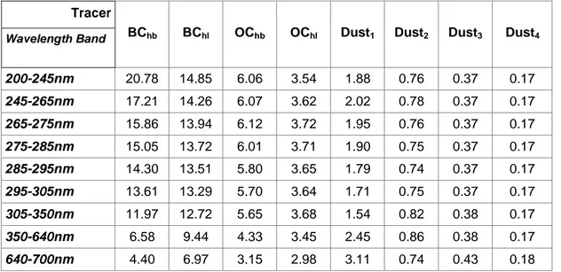
4.1.3 Aerosol emissions and chemistry module parameters ………... 98
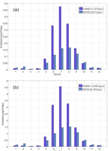
4.1.3.1 The AMMA biomass burning inventory ……… 98
4.1.3.2 The GFEDv2 biomass burning inventory ……… 98
4.1.3.3 Aerosol and dust module setup ……… 98
4.1.4 Internal model variability ……….. 99
4.1.5 Sensitivity tests ……….. 99
4.1.5.1 Testing biomass burning inventories ……… 99
4.1.5.2 Aerosol sea surface temperature feedbacks ……….. 99
4.2 Model validation ………. 100
4.2.1 Surface temperature ………... 100
4.2.2 Precipitation and circulation ……….. 101
4.2.3 Aerosol optical depth ………... 103
4.2.3.1 Temporal comparison ……… 103
4.2.3.2 Spatial Comparison .……….. 104
4.3 Simulated aerosol impacts ……….. 109
4.3.1 Surface radiative forcing ………. 109
4.3.2 Aerosol-induced surface temperature changes ……….. 111
4.3.3 Top-of-atmosphere radiative forcing ………. 111
4.3.4 Atmospheric radiative forcing ………. 112
4.3.5 Surface energy balance ……….. 112
4.3.6 Regional dynamical changes ………. 114
4.3.7 Aerosol-induced precipitation changes ………... 117
4.4 Sensitivity of simulated aerosol impacts ……… 118
4.4.1 GFED sensitivity test results ………. 119
4.5 Conclusions ……… 121
Chapter 5: Variability of aerosol-climate impacts at different timescales –
Interannual to synoptic variability
5.1 Experiment description, model setup and validation ………... 1235.1.1 Model domain and boundary conditions ……….. 123
5.1.2 Aerosol emissions and aerosol module setup ……… 125
5.1.3 Validation of simulated aerosol optical depth ………. 125
5.2 Long-term austral winter aerosol-climate impacts ………... 130
5.2.1 JJAS seasonal average radiative forcing ………. 130
5.2.2 Surface impacts ……….……….. 131
5.2.3 Regional atmospheric dynamical changes ……….. 134
5.3 Interannual variability of seasonal aerosol impacts ………. 134
5.3.1 Interannual variability of aerosol optical depth ……… 135
5.3.2 Aerosol-induced surface temperature changes ……….. 136
5.3.3 Precipitation changes ……….. 138
5.3.4 Association with regional climate drivers ………. 140
5.4 Synoptic variability of aerosol-climate impacts ………. 143
5.4.1 Self-Organising Maps (SOMs) ……….. 143
5.4.2 Applying the SOM technique over southern Africa ……… 143
5.4.3 Synoptic aerosol optical depth variability ……… 147
5.4.4 Simulated radiative forcing variability ……….. 149
5.4.5 Synoptic variability of surface impacts ………. 151
5.4.6 Variability of atmospheric dynamics and precipitation ……….. 153
5.5 Conclusions ……… 154
Chapter 6: Synthesis and perspective
6.1 Synthesis of results ………... 157 6.1.1 Objective one …..………. 158 6.1.1 Objective two …..………. 158 6.1.1 Objective three ...………. 159 6.1.1 Objective four …..………. 160 6.1.1 Summary ………..………. 1616.2 Discussion and Perspectives ……….. 161
6.2.1 Caveats and assumptions ……….. 161
6.2.2 Perspectives ………. 163
Appendix
A A.1 RegCM3 domain sensitivity over southern Africa ……… 165A.2 RegCM3 sensitivity to convective parameterisation ……… 178
Appendix
BB.1 Validation of southern African climate: 1982-2001 ……….. 187
CHAPTER 1
Why aerosols? Why southern Africa?
1.1 Motivation from a global perspective ……… 13
1.2 Motivation at the regional level ………. 15
1.3 Why regional climate modelling? ………..……… 17
1.4
Goals and aims of this study ……….……… 191.1
Motivation from a global perspective
Aerosols affect the earth system in a multitude of ways, by influencing the radiative budget, atmospheric chemistry processes, ecosystem functioning and even human health. Aerosol impacts on the earth-atmosphere energy budget affect global and regional climate by redistributing heat within the atmosphere and influencing atmospheric stability, affecting regional circulation patterns and the hydrological cycle [Chylek and Coakley, 1974; Martin et al., 1990; Dockery et al., 1994; Garstang et al., 1998; Lohmann and Feichter, 2005; Solomon et al., 2007; Ramanathan and Carmichael, 2008].
Light-coloured aerosols, such as sulphate particles, tend to scatter incoming radiation, cooling both the atmosphere and surface by reflecting radiation that would normally have entered the earth system [Chylek and Coakley, 1974; Arimoto, 2001; Sinha et al., 2003; Huang et al., 2007]. On the other hand, dark-coloured aerosols have a somewhat more complex impact, serving both to reflect and absorb incoming radiation. Absorption by these aerosol locally warms the atmosphere but simultaneously also contributes to surface cooling through the conventional ‘surface dimming’ effect [Kaufman et al., 2002; Giorgi et al., 2003; Kinne et al., 2003; Ramanathan and Carmichael, 2008]. Aerosol-induced warming at altitude may serve to decrease cloud cover (termed 'cloud burning') and exacerbate the positive, warming effect by locally reducing relative humidity [e.g. Ackerman et al., 2000; Koren et al., 2004]. In other cases, however, the warming at altitude may also serve to enhance cloud cover particularly if humidity is high and the absorbing aerosol layer lies above a low-level cloud deck [e.g. Johnson et al., 2004; Brioude et al., 2009; Perlwitz and Miller, 2010]. Whether resulting in a positive or negtive radiative forcing, this warming at altitude and the consequent impacts on cloud cover are known as the semi-direct aerosol effects.
In addition, aerosols also indirectly affect the earth’s energy budget by acting as cloud and ice condensation nuclei [Twomey, 1974; Kaufman et al., 2002; Lohmann and Feichter, 2005]. Increasing the aerosol loading generally tends to decrease average cloud and ice droplet size, thus resulting in increased cloud albedo and thickness [Twomey, 1974], as well as an increase in cloud lifetime [Albrecht, 1989], and, depending on the cloud type, also possible delays in precipitation onset and possible increases in precipitation intensity [Kaufman et al., 2002; Lohmann and Feichter, 2005]. Finally, and not to be forgotten, aerosols have numerous non-climatic impacts. They affect regional ecosystems through deposition of micronutrients as well as through the formation of acid rain [e.g.OECD, 1977; Garstang et al., 1998; Piketh et al., 2000; Tyson and Gatebe, 2001; Billmark et al., 2005] and also significantly impact human health, particularly in urban areas [e.g. Dockery et al., 1994; Forsberg et al., 2005; Liu et al., 2009].
Figure 1.1: Radiative forcing estimates of various components of the earth system, as well as the scale at which they dominate and the level of scientific understanding (LOSU) associated with each process [extracted from the IPCC AR4 report, 2007].
The relatively short atmospheric lifetime of aerosols leads to highly heterogeneous distributions through space and time. Partly as a result of this large variability and also because of uncertainty regarding their optical properties, the magnitude of the global aerosol radiative forcing remains highly uncertain [Pilewskie et al., 2003; Kinne et al., 2003; Solomon
et al., 2007]. The most recent International Panel on Climate Change (IPCC) report [2007] suggests that aerosol are likely to have a negative radiative forcing (thus cooling effect) comparable in magnitude to the warming effect of carbon dioxide (CO2). The uncertainty
associated with these estimates is, however, of similar magnitude to the estimates themselves and scientific understanding of these processes is still relatively low (see the well-known IPCC radiative forcing chart in fig. 1.1). At the regional scale, uncertainty in terms of aerosol radiative forcing and associated climate impacts is even greater.
Over the past two decades, awareness of the importance of aerosols on the climate system has grown and a large number and variety of models have been developed as means to estimate aerosol radiative forcing and their impact on climate, ecosystems and human health. In addition, a large number of earth-observing satellite missions have been launched and a wealth of aerosol-related observational data has become available over the past decade. Because of the enormous complexity of aerosol-related processes, some of which are still being discovered, measuring and simulating the aerosol impact on climate is a non-trivial task, no matter what scale is considered: global, regional or local. Models, thoroughly validated with observations are, at present, one of the best-available tools to further our understanding of aerosol impacts and to make better estimations of their radiative effect on the global energy budget.
1.2 Motivation at the regional level
At the regional scale aerosol radiative forcing may be as large or even greater than that of greenhouse gases [e.g. Keil and Haywood, 2003; Kinne et al., 2003]. Over southern Africa, however, the radiative impacts of aerosol and particularly their climatic impacts have been relatively poorly studied. This is especially important for Africa, which has been targeted as one of the most vulnerable regions to global change [Solomon et al., 2007]. Specific, regional-level information is of particular importance in developing regions such as southern Africa, where vulnerability to climate variability is high and the ability to cope and adapt to climatic changes is relatively low. It is thus vital that climate variability and the influence of the regional atmospheric aerosol burden over the subcontinent is better understood and more accurately quantified.
Southern Africa provides the ideal test bed for aerosol-climate studies. Its unique geographical location, climate and biophysical attributes mean that the region is influenced by virtually all aerosol types. The atmospheric aerosol loading is affected by strong seasonal biomass burning [Piketh et al., 1999b; Tyson and Gatebe, 2001; Swap et al., 2003], mineral dust production [Prospero et al., 2002], anthropogenic emissions [Zunckel, 1999; Terblanche et al., 2000] as well as marine aerosol [Piketh et al., 1999a]. Moreover, since most of
southern African lies in the subtropics, below the descending branch of the Hadley Cell, high pressures and subsidence dominate atmospheric circulation patterns for much of the year [Tyson et al., 1996a; Privette and Roy, 2005]. As a result of the high degree of atmospheric stability and anticyclonic circulation patterns associated with these conditions, the regional aerosol burden recirculates and accumulates below expansive stable layers that may stretch over 30° latitude in extent [Cosijn and Tyson, 1996; Tyson et al., 1996a,b]. This is particularly the case during the dry, austral winter season when biomass burning and dust aerosol concentrations are highest. As a consequence of the extensive recirculation, atmospheric aerosol lifetimes over southern Africa are longer than most other regions [Liousse et al., 1996; Tyson et al., 1996b] and the regional aerosol loading is likely to strongly affect the radiative balance over much of the subcontinent [Garstang et al., 1996; Swap et al., 2002a,b; Reason et al., 2006].
Figure 1.2: Map of southern Africa and its component countries, with inset showing its situation relative to the rest of Africa. Depending on the definition, Tanzania may be included as East Africa rather than southern Africa.
In addition, the southern African region also has an important impact on the global atmosphere, with aerosol and trace gases from the region being transported and affecting the atmosphere and climate well beyond the subcontinent [e.g. Fishman et al., 1991; Sturman et al., 1997; Pak et al., 2003]. As an example, evidence suggests that the transport of iron-rich mineral dust aerosol to the southwest Indian Ocean supports the very high biological activity
observed in this area. This activity is associated with a large uptake of carbon dioxide and the region serves as an important carbon sink and is significant in terms of the global carbon budget, and possibly even global climate [Tyson and Gatebe, 2001].
In an effort to better understand southern African aerosols and their impacts over the region two large, multi-disciplinary field campaigns were carried out in 1992 and 2000. These experiments aimed to characterise the regional atmospheric aerosol and trace gas composition as well as to investigate their sources, transport, physical and chemical transformation, their eventual deposition and their eventual influence on regional ecosystems and climate [Swap et al., 2002a,b]. A number of smaller, more local experiments and field campaigns have also taken place throughout the region over the past few decades, contributing to our working knowledge of the region and its atmospheric chemistry [e.g. Kirkman et al., 2000; Jayaratne and Verma, 2001; Martins et al., 2007]. A relatively small number of modelling studies concentrating on southern Africa have also been performed, ranging from global studies with some focus on the region [e.g. Takemura et al., 2002; Abel et al., 2005; Kinne et al., 2006], through to regional climate investigations [e.g. Joubert et al., 1996, 1999; Tadross et al., 2005] and studies of local radiative transfer budgets [e.g. Bergstrom et al., 2003; Jury and Whitehall, 2009].
1.3 Why regional climate modelling?
The climate model era dawned in the late 1970s with the development of global atmospheric models, which were typically run at very coarse resolutions ranging between 5°-7.5°. The need for resolving processes occurring at sub-grid-scale resolution led to the evolution, in the late 1980s, of limited-area models for climate applications. This work was pioneered by Dickinson et al. [1989] and Giorgi [1990], and is essentially based on the idea that a low-resolution global model or gridded observational dataset can be used as lateral boundary forcing for a high-resolution regional model focusing on a specific area of interest (see fig. 1.3 for an idealised depiction of this concept).
Over the years, both global and regional climate models have continued to develop in parallel, as our understanding of the earth system has improved and computing resources have advanced. The current generation of global climate models (GCMs) can run at resolutions as high as up to 50km (some even up to 20km, but with considerable changes to model physics) and most have been coupled to ocean and sea-ice models (AOGCMs), as well as to dynamic vegetation, hydrological and aerosol-chemistry models. The complexity of these models, however, means that simulating at such high resolutions over the long multi-century periods necessary for climate studies is not computationally feasible, and, at present, global models are typically still run at resolutions ranging from ~125-400km. This is
particularly true for global chemistry-climate models, which are extremely computationally intensive and which are generally still run at even lower resolutions (e.g. at ~2ºx 2.5º latitude by longitude).
Regional climate models (RCMs), which are currently run at resolutions varying anywhere between less than 10 to 80km, therefore continue to provide higher spatial information than GCMs [Vannitsem and Chome, 2005; Solomon et al., 2007]. The fine-scale resolution of topography, land-use characteristics and vegetation structure means that RCMS are better able to resolve the local effects these features have on weather and climate more accurately than the current generations of GCMs [Christensen et al., 1997; Joubert et al., 1999; Giorgi et al., 2006]. This high resolution is particularly important for the simulation of aerosol processes, which, as mentioned, are highly heterogeneous in space and time [Simmons et al., 2004].
Figure 1.3: A schematic representation of the horizontal and vertical resolution typical of a regional climate model (RCM).
Over the past two decades RCMs have been widely applied in various studies around the globe. Most studies have concentrated on the northern hemisphere, where, traditionally, the technical capacity for carrying out these studies has been focused. Compared to other regions, relatively few regional modelling studies have been carried out over Africa and a large part of this work has focused on the West African Monsoon region [e.g. Afiesimama et
al., 2006; Konare et al., 2008]. Although some regional climate modelling investigations have been carried out over the southern African region [e.g. Joubert et al., 1999; Hudson and Jones, 2002a; Tadross et al., 2005, 2006], no studies have yet examined the aerosol-climate impacts over the subcontinent using a coupled regional climate-chemistry model. In addition, very few modelling studies have concentrated on climate change scenarios for southern Africa [e.g. Hudson and Jones, 2002b]. Investigating the impact of climate change, and the likely feedbacks of aerosol forcing on this signal, is essential for the southern African region given its vulnerability and relatively low level capacity for mitigation and adaptation [Solomon et al., 2007]. To date, only a very limited number of studies have investigated these impacts.
1.4 Goals and aims of this study
The primary goal of this work is to investigate the direct and semi-direct radiative effects of aerosols on the southern African regional climate. For this purpose, the regional climate model RegCM3, which includes a basic land surface model as well as aerosol-chemistry and mineral dust emission modules, is used. We concentrate on the direct and semi-direct radiative effect of aerosols, since these aspects of aerosol forcing are more completely understood over Africa, at least in terms of the physical nature of such processes, and are thus better formulated in RegCM3. In addition, we focus on the dry austral winter season, since during these months very little precipitation occurs over southern Africa and the indirect aerosol effect is likely to be of little consequence to the regional atmosphere [Swap et al., 2003].
Within this context, the initial step is to validate RegCM3 and its aerosol chemistry module over the southern African region and in particular to assess the degree of uncertainty associated with the parameterisation of certain aerosol processes, such as emission and deposition. Thereafter, the second step is to explore the seasonal average climatic impacts of the atmospheric aerosol burden and to investigate the degree of variability between simulated impacts when using different biomass burning aerosol emissions inventories and different boundary forcing conditions. This is especially important given the high degree of uncertainty still associated with such emissions estimates (ranging up to a factor of two [e.g. Korontzi et al., 2004; Liousse et al., 2010]. Finally, the last step is to evaluate the variability of the various aerosol-climate impacts at different time scales, ranging from the interannual to the synoptic. The possible temporal variability of aerosol-climate impacts is a feature little explored in the literature, but one that is of considerable importance given the multitude of time scales over which aerosol processes act.
To summarise, the main objectives of this work are identified as:
sensitivity to various parameters associated with the online aerosol module;
•
assessing the ability of RegCM3 to reproduce southern African regional climate and especially seasonal atmospheric aerosol characteristics;•
investigating the simulated direct and semi-direct aerosol effects on the regional climate during the austral winter and to explore the sensitivity of model simulated aerosol-climate impacts in response to various aerosol emissions inventories and a forced sea surface temperature-feedback; and•
investigating the aerosol-climate impacts at different time scales, ranging from the interannual to the synoptic scale.This thesis has been developed into five sections to respond to these aims. Chapter two provides a general overview of the literature relevant to this study, including a description of the southern African region, various aerosol processes and the wide range of observations used for model validation. Chapter three includes a description of the regional climate model used, as well as results from a number of sensitivity tests that were carried out to assess model sensitivity over southern Africa. On the basis of these results the best model configuration over the southern African region was chosen. Chapter four is based on work carried out for the article 'Simulation of the direct and semi-direct aerosol effects on the southern Africa regional climate during the biomass burning season', recently published in the Journal of Geophysical Research [Tummon et al., 2010]. This chapter focuses on the climatic impact of biomass burning aerosol during the southern hemisphere winter season over the 2001-2006 period. Chapter five extends this work, covering a 20-year period, specifically aimed at investigating the variability of aerosol impacts at different scales, from the interannual through to the synoptic, as well as to further explore the uncertainty resulting from another, decadal-average emissions inventory. Finally, a summary of the most relevant results as well as perspectives on the investigations carried out completes this work in the final section, chapter six.
CHAPTER 2
Background and introduction
2.1 Southern Africa: a regional description ……….. 22 2.1.1 Regional climate and mean circulation patterns ………. 22 2.1.2 Absolutely stable layers ……….. 26 2.1.3 Recirculation over southern Africa ……… 28 2.1.4 Aerosol plumes exiting the subcontinent ………. 29 2.1.5 Southern African climate variability ……….. 31 2.1.6 Observed temperature and precipitation trends ………. 33 2.1.7 Future climate projections ……….. 34 2.2 Atmospheric aerosol ………. 35 2.2.1 Aerosol formation, particle growth and size distribution ……… 36 2.2.2 Aerosol sources ……….. 37 2.2.2.1 Industrial aerosol ……… 38 2.2.2.2 Carbonaceous aerosol ……….. 39 2.2.2.2.1 Black carbon ……….. 40 2.2.2.2.2 Organic carbon ………. 41 2.2.2.3 Biomass burning ………. 41 2.2.2.4 Mineral dust aerosol ………... 45 2.2.2.5 Marine aerosol ………. 48 2.2.3 Aerosol deposition ……… 48 2.2.3.1 Dry deposition ………. 48 2.2.3.2 Wet deposition ………. 49 2.2.4 Aerosol optical properties ……… 50 2.2.4.1 Aerosol optical depth ……….. 50 2.2.4.2 Phase function ………. 50 2.2.4.3 Single scattering albedo ………. 51 2.2.5 Aerosol-radiation-climate interactions ……… 51
2.2.5.1 The direct aerosol effect ………. 53 2.2.5.2 The semi-direct aerosol effect ..………. 54 2.2.5.3 The indirect aerosol effects ……… 55 2.2.6 Other aerosol impacts ……….. 57 2.3. Aerosol observations ………. 58 2.3.1 Field campaigns in southern Africa ……… 58 2.3.1.1 SAFARI-1992 ………... 59
2.3.1.2 SA’ARI-1994 ……… 60 2.3.1.3 SAFARI-2000 ……….. 60 2.3.1.4 IGAC DEBITS Africa (IDAF) ………. 62 2.3.2 Remote sensing observations ……… 62
2.3.2.1 The Aerosol Robotic Network (AERONET) ……… 63 2.3.2.2 Total Ozone Monitoring System (TOMS) ……… 64 2.3.2.3 Multi-Imaging Spectro-Radiometer (MISR) ………. 65 2.3.2.4 Moderate Resolution Imaging Spectrometer (MODIS) ………. 65 2.4 Regional climate modelling ………... 66 2.4.1 A brief introduction to regional climate models ………. 66 2.4.2 Regional climate modelling studies over Africa ……… 68
2.1 Southern Africa: A regional description
2.1.1 Regional climate and mean circulation patterns
Southern Africa is a diverse and dynamic region in terms of many aspects: culturally, politically, ecologically and climatologically. Landscapes contrast widely, varying from poor to wealthy, stable to fluctuating and rich and fertile to dry and barren. Because of this variety, the subcontinent provides a unique and challenging environment in which to investigate the multitude of components that make up the regional coupled atmosphere-ocean system.
Geographically speaking, southern Africa is most frequently described as the region south of approximately 10ºS [Tyson and Preston-Whyte, 2000]. Much of the subcontinent lies on an elevated plateau at altitudes well in excess of 1000m, while the coastal margins are narrow, particularly in the south and southeast. Vegetation coverage essentially follows the north-south precipitation gradient, with the northern, wetter parts being dominated by broad-leafed, deciduous woodlands and dry forests. This progressively transitions into semi-arid, fine-leafed savannahs and grasslands that extend through most of the southern, drier parts of the region [Privette et al., 2004; Shugart et al., 2004]. To the very southwest, where semi-arid to arid conditions prevail, vegetation cover is sparse and shrubland or semi-desert vegetation dominate [Privette and Roy, 2005].
Most of southern African is situated in the subtropics, experiencing warm, dry winters and hot, humid summers. The regional atmospheric circulation is dominated by the semi-permanent high-pressure systems that constitute the general circulation of the southern hemisphere in this zone (see fig. 2.1.1). Except for at the surface, circulation patterns are anticyclonic for much of the year, the result of subsidence associated with the descending branch of the southern Hadley Cell [Tyson and Preston-Whyte, 2000; Reason et al., 2006]. These
circulation patterns are most frequent during the austral winter, from May through September, when the southern hemisphere Hadley Cell moves northwards and land surface temperatures are cooler. During this season the Inter-Tropical Convergence Zone (ITCZ), associated with the convergence of the northern and southern Hadley Cells is situated in the northern hemisphere.
As the year progresses and the surface warms, the southern Hadley Cell and ITCZ migrate southwards. This signals the beginning of the rainy season for most of southern Africa in October and November. On average, the ITCZ extends to about 15-17ºS, although this may vary by several degrees latitude from year to year [Torrance, 1972]. In some years it is situated further north than average, near 10-12ºS, and during these seasons southern African rainfall tends to be below normal since the comparatively dry south-easterly trades that form the southerly branch of the ITCZ dominate regional circulation patterns. In other years, the ITCZ strays unusually far south, sometimes reaching as far as 20ºS, bringing with it anomalously moist air and heavy rain to these regions [McHugh and Rogers, 2001]. Outside of the summer season rainfall may occur sporadically, but generally contributes relatively little to annual precipitation totals [Tyson and Preston-Whyte, 2000; Shugart et al., 2004].
Figure 2.1.1: (a) Summer and (b) winter average sea-level pressure (contours) and winds (vectors) over Africa. The stippled (dashed) line indicates the climatological location of the Inter-Tropical Convergence Zone (Zaire Air Boundary). Average vertical circulation patterns are presented on the left of each figure. [Following Nicholson and Grist, 2003].
A secondary convergence feature, the Zaire Air Boundary (ZAB; alternatively known as the Congo Air Boundary) originating from the South Atlantic, also influences circulation and precipitation patterns, particularly over the western half of the subcontinent [Tyson and
Preston-Whyte, 2000; McHugh and Rogers, 2001]. The ZAB affects southern Africa largely only in the austral summer when it extends from southwest to northeast traversing the subcontinent at similar latitudes to the ITCZ and eventually converging with this feature over eastern central Africa [Tyson and Preston-Whyte, 2000; see fig. 2.1.1]. As this air stream moves eastward over the Congo basin and flows toward the higher elevations of eastern Africa it cools adiabatically and brings abundant rainfall to these regions [Torrance, 1972; Nicholson, 1996]. The seasonal average position of the ITCZ and ZAB in both the southern hemisphere summer (January) and winter (July/August) seasons can be seen in figure 2.1.1(a) and (b) respectively.
Anticyclonic circulation returns to dominate the regional atmosphere as the rainy season comes to an end in March and April and the ITCZ begins its migration back towards the northern hemisphere. As the land surface cools and dries a surface temperature gradient is established between the semi-arid southern parts of the subcontinent and the sub-humid, perennially vegetated regions further north. From August onwards this temperature gradient induces a seasonal jet system, the southern branch of the African Easterly Jet (AEJ-S), which is usually persistent through until December [Nicholson and Grist, 2003]. Over the continent this jet has a well-defined core centred near 5º south at an altitude of approximately 700hPa, but over the adjacent Atlantic Ocean, the AEJ-S is situated closer to the equator and is neither as persistent nor as strong as over land. During the late summer (January to March) the jet degenerates as the ITCZ shifts back into the southern hemisphere and the precipitation it produces over the southern semi-arid regions reduces the strong surface temperature gradient that contributes to the formation of this jet [Nicholson and Grist, 2003].
The south-western-most tip of the subcontinent is the only region that does not experience a summer rainfall regime. Closer to the mid-latitudes than the tropics, this small portion of southern Africa receives maximum precipitation in the austral winter when the westerlies that dominate the temperate southern hemisphere regions strengthen and expand equatorward [Cosijn and Tyson, 1996; Shugart et al., 2004]. Rainfall is significant from July through to November, when the mid-latitude jet stream, a core feature of the westerly circulation patterns, reaches its most northerly position centred near 25°S [Garstang et al., 1996; Tyson and Preston-Whyte, 2000]. Similar to the AEJ-S, this jet stream is maintained by a strong meridional temperature gradient, but on this occasion one that exists in the mid- and upper troposphere.
Circulation patterns over the adjacent Atlantic and Indian Oceans are more consistent than over land, with anticyclonic conditions prevalent throughout the year. Although these systems undergo seasonal intensification and shift both in terms of latitude and longitude from season to season, they effectively remain a strong feature of the high-pressure systems that dominate the subtropical belt [Tyson and Preston-Whyte, 2000]. On the daily scale, the
Atlantic high may ridge east and south of the continent, sometimes leading to the ‘budding’ off of a separate high that then migrates eastward to the Indian Ocean. These ridging anticyclones strongly affect the weather of the subcontinent, particularly during the austral summer when the ocean high-pressures are most intense [Tyson and Preston-Whyte, 2000].
Figure 2.1.2: Mean austral summer (a; December to February) and winter (b; June to August) zonal wind (left sections) and mass flux (right sections). Areas where easterly zonal winds dominate are stippled grey (left sections) and dotted lines indicate mass flux contours less than 1012gm.s-1 (right sections). [Following Tyson and Preston-Whyte, 2000].
A number of the above-mentioned features are also evident in fig. 2.1.2, which shows the mean summer (December-February) and winter (June-August) zonal wind (left) and mass flux (right) profiles of the Southern Hemisphere. Seasonal average surface pressure (left) and meridional pressure profiles (right) are also shown in this figure. The latitudinal position of the
southern Hadley cell and the climatological region of subsidence (stretching over much of southern Africa, especially in winter) are clear. The position of the mid-latitude westerly jet is also evident near 200hPa during both seasons, as are the semi-permanent high pressure systems over the Atlantic and Indian Oceans.
2.1.2 Absolutely stable layers
The predominance of anticyclonic circulation and large-scale subsidence over southern Africa results in clear, dry conditions and adiabatic warming occurs throughout much of the regional atmosphere [Tyson and Gatebe, 2001; Kirkman et al., 2000]. The clear conditions mean that during the day the rate of incoming solar radiation is high, while at night significant cooling can occur. This, in combination with the adiabatic warming that occurs, creates the potential for a very a stable atmospheric thermodynamic structure, ideal for the generation of absolutely stable layers throughout the troposphere [Tyson et al., 1996].
Absolutely stable layers are defined as regions where the environmental lapse rate is less than the saturated adiabatic lapse rate [Tyson et al., 1996]. At any one time, up to four such layers may be present simultaneously over southern Africa [Tyson et al., 1996; Tyson and Gatebe, 2001]. These layers confine both horizontal transport and vertical diffusion of aerosols and trace gases (including water vapour) over the entire subcontinent and lead to an accumulation of both anthropogenic and biogenic products in the regional atmosphere [Tyson et al., 1996; Freiman and Tyson, 2000; Tyson and Gatebe, 2001; Freiman et al., 2002]. The longevity and ubiquity of these features is unique to southern Africa, and they are of considerable consequence, particularly in terms of regional atmospheric chemistry [Swap et al., 2002a,b].
The lowest of these absolutely stable layers occurs at approximately 850hPa, and is associated with the top of the mixing layer over the narrow coastal regions. This layer does not exist over the central plateau region since the plateau is, for the most part, higher in altitude than this level [Cosijn and Tyson, 1996]. In addition to anticyclone-associated subsidence, the development of the 850hPa absolutely stable layer is also affected by ocean-atmosphere heat fluxes, topographical influences, as well as sea breezes [Freiman and Tyson, 2000]. The second absolutely stable layer, which forms near 700hPa, occurs over the entire southern African region and is associated with the top of the mixing layer over much of the central plateau [Kirkman et al., 2000]. Both of these lower layers are frequently disrupted by the passage of low-pressure systems, which promote vertical mixing of aerosols and trace gases up to the 500hPa level. On average these low-pressure systems pass every six to seven days [Preston-Whyte and Tyson, 2000; Tyson et al., 1996].
The third absolutely stable layer forms preferentially at 500hPa and is the most persistent, being present on approximately 78% of the days of the year and at times for as long as up to 40 consecutive days [Cosijn and Tyson, 1996; Tyson et al., 1996; Piketh et al., 1999a; Freiman and Tyson, 2000; Freiman and Piketh, 2003]. Due to its enormous spatial extent (often covering up to 30º latitude) and the dense haze that is often trapped below this layer, it is commonly referred to as the ‘African haze layer’ [Tyson et al., 1996; Garstang et al., 1996]. Above this layer the air is remarkably clear, with aerosol number concentrations dropping by at least two orders of magnitude from between 3000-10000/cm3 in the haze layer to between 10-90/cm3 above it [Tyson and D'Abreton, 1998]. The fourth and highest level occurs at approximately 300hPa in the upper troposphere and is of greater relevance to the vertical and horizontal transport of ozone than to aerosols and trace gases [Tyson et al., 1996].
Somewhat surprisingly, absolutely stable layers are common even in the wet summer season on no-rain days, occurring on over 70% of all days over South Africa [Cosijn and Tyson, 1996]. Only deep convection or unstable barotropic easterly disturbances occurring during the rainy season cause a break down of the stable layers at all four levels simultaneously. These processes induce extensive vertical mixing and also enhance aerosol transport out of the region [Cosijn and Tyson, 1996; Garstang et al., 1996; Freiman et al., 2002]. Equatorward of 15°S the stable layers rise in altitude and ultimately disappear in the convective region of the ITCZ [Garstang et al., 1996].
Figure 2.1.3: The occurrence of absolutely stable layers on no-rain days over South Africa averaged over the seven-year period 1986-1992 from a total of 2925 radiosonde ascents at (a) nine different stations and (b) averaged over different periods of the year (% occurrence). The depth of each layer is indicated by the vertical extent of each box and vertical lines give the standard deviation of base height. PI denotes Pietersberg, PA Pretoria, BE Bethlehem, BL Bloemfontein, UP Uppington, SP Springbok, CT Cape Town, PE Port Elizabeth and DB Durban. [Following Cosijn and Tyson, 1996].
The average position and frequency of occurrence of the four absolutely stable layers is shown in fig. 2.1.3 for nine stations in South Africa where radiosonde measurements were taken from 1986-1992. The altitude of all four (three) layers over the coastal (plateau) stations is clear (fig. 2.1.3(a)), as is the very high frequency of occurrence throughout the year (fig. 2.1.3(b)). Also presented are the average vertical depth and variability of base height of each level (vertical lines extending from the bottom of each box).
On occasion, absolutely stable layers may merge for one or several days, causing the aerosols trapped below these layers to mix. For example, merging of the 700 and 500hPa layers has been found to occur as frequently as 35 and 25% of the time in summer and winter respectively [Freiman and Tyson, 2000]. Alternatively, if a particular layer is not present, aerosols are also vertically mixed up to the next stable layer [Freiman et al., 2002]. In general, all the stable layers are relatively shallow features, seldom exceeding 1km in depth [Cosijn and Tyson, 1996]. Interestingly, despite large differences in synoptic conditions and their respective aerosol accumulation mechanisms, the vertical structure of the southern African lower troposphere remains remarkably similar, with all major absolutely stable layers present in similar vertical positions and extending over similar regions horizontally [Stein et al., 2003].
2.1.3 Recirculation over southern Africa
The dominant anticyclonic circulation patterns also result in a significant amount of recirculation of air, at local, regional and subcontinental scales [Tyson et al., 1996; Piketh et al., 1999b; Tyson and Gatebe, 2001]. Recirculation can be defined as the recycling of air, or transport that returns an air parcel to its point of origin from the opposite direction to which it left, having rotated or recurved in cyclonic or anticyclonic circulation systems [Tyson and Gatebe, 2001; Torres et al., 2002]. On average over the year, approximately 54% of all air is recirculated at least once over the subcontinent before exiting to either the Atlantic or Indian Ocean. Recirculation is induced by either stationary continental high pressure systems, which occur on average 40% of the year (maximum in July (70%) and minimum in January, (15%)), or with the passage of transient ridging anticyclones, which commonly follow in the path of mid-latitude low-pressure systems [Tyson et al., 1996; Piketh et al., 1999a; Torres et al., 2002].
Recirculation also occurs, although to a lesser degree, from the Atlantic and Indian Oceans back towards the subcontinent. The air thus returns containing marine aerosol, which may have become incorporated into the air parcel during transport [Garstang et al., 1996; Tyson and D'Abreton, 1998; Piketh et al., 1999a; Eck et al., 2003]. Recirculation back towards the subcontinent is biased towards the west coast, where, at 15°E, approximately 35% of air
recirculates back towards the east. In contrast, over the east coast, at 35ºE only 13% of air recirculates back towards the continent [Garstang et al., 1996].
The atmospheric lifetime of a particular aerosol species depends largely on its physical and chemical properties, as well as its place, time and height of release. As a consequence of the high degree of recirculation, aerosol residence times over southern Africa are considerably longer compared to most other regions [Tyson et al., 1996; Liousse et al., 1996]. The climatological mean recirculation period over southern Africa is approximately 7-10 days, however, on occasion air has been found to recirculate over the subcontinent as long as 20 days. Recirculation thus maintains high aerosol loads over the region [Swap and Tyson, 1999], particularly during winter, when there is little humidity or precipitation [Tyson et al., 1996; Tyson and D'Abreton, 1998; Piketh et al., 1999a]. Importantly, the maintenance of cloud-free conditions and high-levels of insolation associated with the prevalent anticyclonic circulation patterns also enhance heterogeneous photochemical transformations of airborne species [Swap et al., 2003].
2.1.4 Aerosol plumes exiting the subcontinent
Despite the high degree of recirculation and the long atmospheric lifetime of aerosols over the southern African subcontinent, a significant quantity of aerosol are transported offshore from the region to the adjacent Atlantic and Indian Oceans in large plumes before deposition occurs [Tyson and D'Abreton, 1998; Piketh et al., 1999a]. In fact, little material is deposited during transport over the continent, with aerosol concentrations in the plumes remaining fairly constant from the regional interior through to the coastal areas [Tyson and D'Abreton, 1998].
The location of the two major exit pathways depends on the relative position of the semi-permanent anticyclone over the subcontinent, but is generally restricted to south of approximately 10°S [Tyson et al., 1998; Tyson and D'Abreton, 1998]. The plumes vary in depth and form depending on the prevalent synoptic conditions, but always lie above the marine boundary layers of both oceans, which occur between the surface and approximately 1.5km above sea level around most of the southern African coast [Tyson and D'Abreton, 1998]. The plumes are complex in structure, simultaneously being made up of in- and out-flowing air streams, which may either lie very close to each other or be separated by hundreds of kilometres [Tyson and D'Abreton, 1998].
Approximately 75% of all southern African air exits via the Indian Ocean plume, which can reach almost 1000km in width [Tyson and D'Abreton, 1998; Piketh et al., 1999a; see fig. 2.1.4]. This plume is a major feature not only of the regional atmosphere but also of the southern hemisphere. It transports an estimated 45 million tons of aerosol each year and
plays a significant role in large-scale, inter-regional aerosol transport [Tyson and Gatebe, 2001]. The air and particulate matter it contains is frequently transported to Amsterdam Island [Moody et al., 1991] and, on occasion even as far as Australia and New Zealand [Sturman et al., 1997; Pak et al., 2003]. The Indian Ocean plume exits the subcontinent with its core situated near 31°S at an altitude of approximately 750hPa [Piketh et al., 1999a]. As the air moves offshore and eastwards, it rises, reaching up to 450hPa, before re-descending to near the surface over the central Indian Ocean at approximately 70°E [Tyson and Gatebe, 2001; Torres et al., 2002]. Deposition into the southern Indian Ocean occurs throughout transport by gravitational settling and precipitation processes. The plume occurs most frequently in winter (72% of all days from May-August), whilst occurring only 33% of all days in summer (November-February) [Tyson and D'Abreton, 1998].
Figure 2.1.4: Generalised atmospheric transport pathways over southern Africa, including the large Indian Ocean and smaller Atlantic Ocean plumes and recirculatory structures. [Following Tyson and Preston-Whyte, 2000].
Although the frequency of occurrence of air transport towards the Indian Ocean does not vary significantly from year to year, there appear to be significant differences in the plume structure and position from year to year as a result of the different circulation patterns typical of wet and dry conditions [Garstang et al., 1996]. A clearly defined Indian Ocean plume was visible during the SAFARI-92 experiment (a dry year), whilst during SAFARI-2000 (a wet year) the plume was considerably more diffuse. It is likely that diminished strength of the mid-latitude westerlies and the increased recirculation that occurs during dry years contribute to
these differences [Garstang et al., 1996; Swap et al., 2003; more about the SAFARI campaigns in section 2.3].
A series of events leads up to Indian Ocean outflow events. Initially, a high pressure anticyclonic system or col region forms over the subcontinent during which aerosols accumulate over the region [Stein et al., 2003], then the passage of low pressure system travelling in the westerlies induces offshore flow and the atmosphere is effectively cleansed as unpolluted marine air is advected over the region and the aerosol-laden air exits the subcontinent towards the Indian Ocean. Aerosols are also rained out if precipitation occurs in association with the cold front.
As a result of the asymmetrical situation of the semi-permanent continental anticyclone over southern Africa, a considerably smaller percentage of aerosol get transported offshore to the Atlantic Ocean [Tyson and Gatebe, 2001; again see fig. 2.1.4]. The Atlantic Ocean plume occurs under two different synoptic situations. Firstly, if a quasi-stationary easterly wave is present over the subcontinent, aerosol material is transported to the equatorial Atlantic from the coast of Angola [Swap et al., 1996; Torres et al., 2002]. Or, secondly, if a transient ridging high passes over the region, air gets transported out to the southern Atlantic Ocean off the coast of Namibia [Kirkman et al., 2000]. Direct transport to the equatorial Atlantic Ocean occurs almost exclusively in summer [Freiman and Piketh, 2003], when easterly waves and ridging anticyclones are most frequent. In both cases, as air moves off the coast and westwards it subsides rapidly as a result of the equatorward geostrophic flow along the eastern margin of the South Atlantic anticyclone. As a result, most aerosols are deposited to the surface before reaching the meridian of 10°W. The flux of aerosols exiting to this region has been estimated at approximately 29 million tons per year [Tyson and Gatebe, 2001].
2.1.5 Southern African climate variability
Southern Africa is characterised by a high degree of interannual and interdecadal climate variability, especially in the western regions [Tyson 1986; Mason and Jury, 1997; Tyson and Gatebe, 2001; Hudson and Jones, 2002a]. Interannual variability is dominated largely by sea surface temperature (SST) variability [Entekhabi and Nicholson, 1988; Mason 1997; Jury et al., 1996; Rocha and Simmonds 1997a,b; Todd and Washington, 2004; Washington and Preston, 2006] and the El-Niño Southern Oscillation (ENSO), which affects the southeastern parts of the subcontinent and East Africa most strongly [Janowiak, 1988; Ropelewski and Halpert, 1996; Reason, 2002; Jury et al., 2004].
In terms of SSTs Mason [1990] showed, that at least over South Africa, SSTs in the South Atlantic explained the greatest amount of variance in rainfall throughout the year, while
variability in southwest Indian Ocean SSTs, which is statistically independent of ENSO, has also been found to influence southern African rainfall variability significantly [Washington and Preston, 2006]. These latter authors found that an enhanced poleward SST gradient in the southwest Indian Ocean is associated with extreme dry years, whilst a weakened gradient is associated with some extreme wet years [Washington and Preston, 2006].
In terms of the ENSO, El Niños (La Niñas) generally induce warm and dry (cool and wet) conditions over much of southeastern Africa. In East Africa the reverse is true, with El Niños (La Niñas) being linked with flooding (drought) [Janowiak, 1988; Ogallo, 1988; Kiladis and Diaz, 1989; Ropelewski and Halpert, 1996]. The ENSO signal is thought to be communicated from the tropics to the extra-tropics through SST changes, particularly from the Indian Ocean [Nicholson and Kim, 1997; Richard et al., 2001], as well as through the atmosphere, as an ‘atmospheric bridge’ [Richard et al., 2000; Richard et al., 2001]. This results in a lag between the observed timing of ENSO impacts in the tropics and mid-latitudes. As a consequence of the circulation changes induced around the globe, the subtropical westerly jets shift equatorward (poleward) and tend to intensify during El Niño (La Niña) events [e.g. Horrell and Wallace, 1981; Sinclair et al., 1997]. Warm and cool ENSO events occur with a periodicity of between three to seven years, peaking around three to four years [Janowiak, 1988; Ropelewski and Halpert, 1996; Tyson and Gatebe, 2001].
Interannual variability over southern African has also been linked with the North Atlantic Oscillation (NAO) [Rogers, 1984; McHugh and Rogers, 2001; Jury, 2009]. During positive NAO phases the Icelandic low-pressure system deepens, while the high-pressure over the Azores region to the south strengthens [Hurrell, 1995]. The NAO has a mean period of between 7.3-8 years and has been observed in rainfall patterns [Jury, 2009], air pressure fields as well as upper-level zonal winds [Hurrell, 1995]. The NAO is exhibited through five elongated bands of alternating zonal wind anomalies extending from the Arctic to equatorial Africa [McHugh and Rogers, 2001]. When the NAO is positive (negative) the most southerly band exhibits anomalous westerly (easterly) flow and divergence (convergence) occurs over southeastern Africa and the region experiences anomalously wet (dry) summers [McHugh and Rogers, 2001; Jury, 2009]. These shifts in zonal winds appear to be related to movement of the ITCZ, which shifts southward (northward) when the NAO is positive (negative) [McHugh and Rogers, 2001].
The Antarctic Oscillation (AAO), alternatively known as the Southern Annular Mode (SAM), is essentially the southern hemisphere equivalent of the Northern Annular Mode (NAM), to which the NAO is closely related. Positive AAO phases are associated with a stronger pressure gradient between mid- and high-latitudes, resulting in a strengthening of the westerlies as well as anomalously warm temperatures in the mid-latitudes but unusually cool temperatures over the Antarctic [Thompson and Wallace, 2000; Thompson and Solomon,