UNIVERSITE DE TOULOUSE III PAUL SABATIER
UFR Physique, Chimie et Applications Sciences de la Planète et de l'Univers
THÈSE
en vue de l'obtention du
DOCTORAT DE L'UNIVERSITE DE TOULOUSE
délivré par l'Université Toulouse III Paul Sabatier
Discipline:
Physique de l'Atmosphère
présentée et soutenue par
Julia HIDALGO RODRIGUEZ
Titre:
UNE APPROCHE OBSERVATIONNEL, NUMERIQUE ET THEORIQUE A LA
CIRCULATION DE BRISE URBAINE DIURNE POUR LES VILLES CONTINENTALES
Sous la direction de:
Valery MASSON
et la codirection de:
Luis GIMENO PRESA
Soutenue le 7 avril 2008 devant le jury composé de:
M. Jean-Philippe GASTELLU
Président
Mme. Sue GRIMMOND
Rapporteur
M. Alberto MARTILLI
Rapporteur
M. Philippe DROBINSKI
Examinateur
M. Valery MASSON
Directeur de thèse
Contents
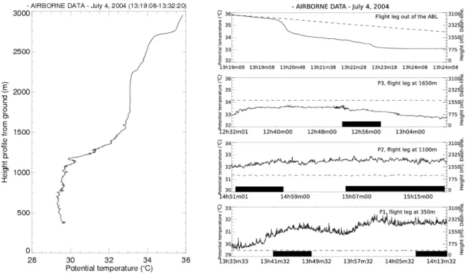
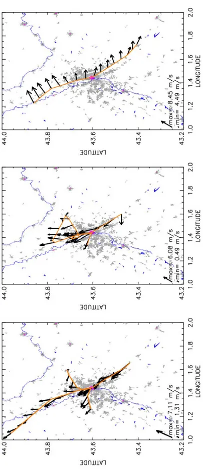
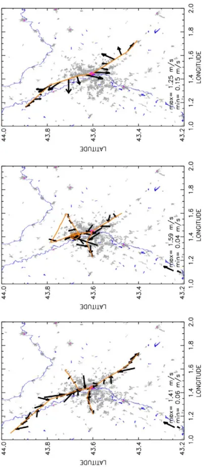
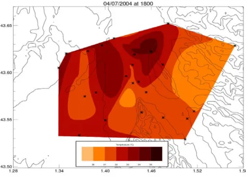
Acknowledgments pg 7 Introduction (fr) pg 9 Introduction (en) pg 13 Chapter 1: Convective boundary layer thermodynamics in urbanized environments pg 17 1. The Atmospheric Boundary Layer pg 17 1.1 Definition and structure pg 17 1.2 ABL features and its meteorological framework pg 19 1.2.1 ABL classification pg 19 1.2.2 Convective ABL pg 20 1.2.3 Vertical fluxes in the CBL pg 22 1.2.4 Air quality in CBL pg 23 1.3 ABL roles at the “global” and “local” scales pg 25 1.4 Thermal circulation dynamics pg 26 2. ABL specificities in urban environments pg 27 2.1 The Urban Boundary Layer pg 27 2.1.1 Definition pg 27 2.1.2 The urban boundary layer height pg 28 2.2. The Urban Heat Island pg 29 2.2.1 Diurnal cycle pg 29 2.2.2 The UHI is modified in function of the meteorological context pg 30 2.2.3 Causes of the UHI generation pg 312.3 Urban impact on the Surface Energy Balance pg 32 3. The UrbanBreeze Circulation pg 34 3.1 General features of wind dynamics in the urban boundary layer pg 34 3.2 Urbanbreeze. Terminology and definition pg 35 3.3 Motivations and approaches of this study pg 36 Chapter 2: The CAPITOUL campaign. An Experimental Approach to the UrbanBreeze Circulation pg 39 UrbanBreeze Circulation during the CAPITOUL Experiment: Experimental Data Analysis Approach 1 Introduction pg 42 2 Observational Network pg 44 2.1 Surface Network in the Area of Study pg 44 2.2 Boundary layer Instrumentation pg 45 3 Meteorological context of this IOP pg 46 4 Temporal and spatial relations between thermodynamics fields and surface features pg 47 4.1 Surface Energy Balance (SEB) pg 48 4.2 Urban Heat Island pg 50 5 The Urbanbreeze circulation pg 51 5.1 Vertical structure of the ABL pg 51 5.2 Identification of the urbanbreeze circulation by the analysis of the aircraft data pg 53 5.2.1 Flight description pg 53 5.2.2 Potential temperature analysis pg 53 5.2.3 Wind field analysis pg 54 5.3 TimeEvolution of the breeze pg 55 6 Conclusions pg 56 References pg 59 List of Tables and Figures pg 63
Chapter 3: Modelling the UrbanBreeze Circulation pg 75 UrbanBreeze Circulation during the CAPITOUL Experiment: Numerical Approach 1 Introduction pg 78 2 Numerical simulations description pg 79 3 Regional Forcing Validation pg 81 3.1 Observational Network pg 81 3.2 Horizontal wind field pg 81 3.3 Potential temperature and water vapour mixing ratio pg 82 4 Temporal and spatial relations between thermodynamics fields and surface parameters pg 82 4.1. Surface Energy Balance (SEB) pg 82 4.2. Nocturnal and diurnal surface heat and humidity islands pg 83 5 Vertical Boundary Layer Development. Urbanbreeze circulation pg 85 5.1. Urban dynamical impact in the morning pg 85 5.2 Perturbation on potential temperature in the ABL pg 86 5.3 The Urbanbreeze circulation pg 86 5.4 TimeEvolution of the Breeze pg 87 6 Conclusions pg 88 Appendix pg 89 References pg 92 List of Figures pg 95 Chapter 4: Theoretical approach: Scaling the daytime UrbanBreeze Circulation pg 105 Scaling the daytime urbanbreeze circulation 1 Introduction pg 109 2 Physics of the problem pg 111 2.1 Current theory relating to the nocturnal UHI and the urbanbreeze pg 111 2.2 Daytime UHI and urban breeze: environment description pg 112 2.3 Daytime UHI and urban breeze: scaling laws pg 113 3 Description and validation of numerical experiments pg 114
4 Scaling the daytime Urban Breeze Circulation pg 116 4.1 Simulated UHI and urban breeze features pg 116 4.2 A new set of scaling laws pg 117 4.2.1 Scaling the daytime UHI pg 117 4.2.2 Scaling the maximum and minimum radial and vertical velocities pg 117 4.2.3 Scaling the vertical profiles of the urbanbreeze circulation pg 118 5 Conclusions pg 119 References pg 122 List of Figures pg 127 Final Conclusions and Pespectives pg 133 Conclusions Finales pg 137 Annexe 1 pg 141 The Canopy and Aerosol Particle Interactions in TOulouse Urban Layer (CAPITOUL) experiment 1 Introduction pg 142 2 Objectives of the campaign pg 144 2.1 Comprehension of urban surface – atmosphere exchanges pg 144 2.2 Structure and development of the urban boundary layer pg 145 2.3 Transformation of urban aerosols pg 146 2.4 Heterogeneity of urban surface temperatures pg 146 2.5 Short distance dispersion pg 147 3 Experimental network pg 147 3.1 Measurement strategy pg 147 3.2 Yearlong measurements pg 148 3.3 Intensive Observation Periods pg 152 4 First results pg 155 4.1 Intraannual variability of the surface energy balance (SEB) pg 155 4.2 Anthropogenic fluxes pg 156 4.3 Urban breeze circulation: observation and simulation pg 157
4.4 Urban fog pg 157 4.5 New insights on urban aerosol pg 158 4.6 Spatial, annual and diurnal heterogeneities of the surface temperature field pg 159 4.7 Evaluation of dispersion modelling pg 160 5 Conclusions pg 160 References pg 163 List of Tables pg 171 List of Figures pg 175 Complete Bibliographic References pg 189 Additional documents: Abstract (fr) pg 215 Abstract (en) pg 216
Agradecimientos Remerciements and
Acknowledgements...
Je te remercie, Valery, pour la direction de ce travail, pour ton temps, tes conseils, ton savoir faire, à ne pas oublier nonplus... la promenade en avion sur les Pyrénées. Gracias Luis, por proporcionarme los medios para compaginar el trabajo entre Toulouse y Orense. Gracias por esta codirección y cofinanciación fructíferas. Merci Joël, je suis passée par trois de tes équipes depuis mes debuts dans la Recherche. Ton appui dans chaque pas a été essentiel. Merci pour la confiance que tu m'as accordée. Je remercie également la direction du CNRM pour avoir appuyé la collaboration avec l'Université de Vigo, et avoir ainsi permis le déroulement de cette thèse. Thanks to the reviewers and examinators who offered a critical review that significantly enhanced our appreciation of the problem treated here and the qualitty of this manuscript. Je tiens à remercier spécialement mon équipe (TURBAU) pour m'avoir accueilli pendant ces trois ans. Les allerretour entre la France et l'Espagne n'ont pas perturbé mon sentiment d'appartenir au groupe. Un merci spècial à tous ceux qui sont passés par le bureau 216. Je remercie également Arnaud Mequignon qui m'a soutenu et permis de bien démarrer dans cette aventure. Merci Arnaud. Je ne peux pas oublier aussi que j'ai été bien soutenue par les équipes d'instrumentation (4M et TRAMM), de modélisation (MESONH), d'informatique et d'administration. A tous un grand merci pour votre disponibilité et professionnalisme. Equipo FT2DC, que evolucionó a FAO9 y que seguro seguirá creciendo. Fué un periodo de retorno para mi y de nuevas aventuras para varios de vosotros. Para los que me acompañasteis insitu y para los que lo hicisteis desde la distancia, gracias por todo. Fred, Anne, Suzanne, Olivier, Bernard, Mag' et à tous ceux que je ne cite pas mais qui sont dans ma pensée, merci pour les pauses café, les coinches (même si je n'ai jamais appris), les randos faciles... les bons moments qui ont fait de Toulouse une ville remplie de bons souvenirs. Gracias también al grupo de Español y las comidas de cada miércoles.A mi familia, para la no todo cabe en un solo gracias ni una sola línea. Por acompañarme, apoyarme, aconsejarme, en este día, en la distancia, la cercanía y... mucho más.
a todos gracias, Julia Hidalgo
Introduction
D'un point de vue social, économique et météorologique, l'environnement urbain est un système complexe qui mérite, de nos jours, l'attention d'une communauté scientifique multidisciplinaire. L'expansion urbaine comme tendance démographique dominante La fraction de la population mondiale vivant dans les zones urbaines n'a pas cessé d'augmenter au vingtième siècle, de telle sorte que des économistes tels que L. R. Brown définissent l'urbanisation comme l'une des tendances démographiques contemporaines dominantes (Brown, 2001). La population urbaine s'accroît trois fois plus rapidement que la population rurale (Nilsson et al., 1999). Vers 2007, la population humaine a atteint un seuil critique, et à partir de cette date plus de la moitié de la population du monde vit dans des environnements urbains, faisant de nous, pour la première fois, une espèce urbaine (Brown, 2001). L'UNEP (Programme des Nations Unies pour l'Environnement) s'attend à une croissance de la population urbaine de 2% par an jusqu'en 2015. Il a été estimé que 60% de la population du monde résidera dans des zones urbaines d'ici à 2025 (Platt, 1994a). L'urbanisation comme noeud d'échange économiqueLes villes forment un réseau de centres concurrentiels qui constituent les points de référence physiques pour la mondialisation que nous connaissons aujourd'hui. Les zones urbaines tirent la croissance économique mondiale et, en même temps, constituent d'un point de vue social et environnemental un système anthropogène des plus vulnérables (SanchezRodriguez et al., 2004).
Les insuffisances dans le niveau de vie urbain comme le chômage, la faiblesse des services publics et les dégradations environnementales sont communes dans la plupart des villes. La vulnérabilité face à des
événements météorologiques ou climatiques est l'un des problèmes majeurs (FCMR222004). Les changements environnementaux globaux ont des conséquences potentiellement graves: influence sur la santé et le confort des habitants, coûts énergétiques (Fusaro, 2007), qualité de l'air et niveaux de visibilité (Wu et al., 2006; Mikley et al., 2004), disponibilité et qualité de l'eau, services écologiques, loisirs, et qualité de la vie générale. Une prévision exacte des caractéristiques du climat urbain est d'une importance première pour réduire les pertes économiques et garantir la sûreté des citadins. Prévision à mésoéchelle / Nowcasting: un outil essentiel
La météorologie urbaine est une approche spécialisée et interdisciplinaire pour étudier les interactions environnementales des communautés urbaines, en fournissant une réponse intégrée à ces demandes. Plusieurs conférences internationales sur le climat urbain ont été tenues depuis la fin des années 1960. Finalement en 2000, la communauté scientifique s'est organisée dans l'Association Internationale pour le Climat Urbain (IAUC). Cette structure regroupe des représentants de l'ensemble de la communauté du climat urbain et organise une conférence internationale tous les trois ans. À mesure que la résolution des modèles de mésoéchelle augmente, les techniques de prévision et de nowcasting appliquées à des domaines locaux/regionaux sont de plus en plus plus utilisées pour développer des protocoles améliorés de prise de décision. La prévision à mésoéchelle est utilisée lors de dégagements toxiques dans l'atmosphère. Les actions sont plus utiles quand elles peuvent être mises en application et mises à jour rapidement, avec des temps de réponse de 15 minutes ou moins (Dabberdt et al., 2000). Quand les modèles globaux prévoient des changements externes ou globaux importants, un run supplémentaire à l'échelle régionale peut être effectué pour atténuer les pertes dues à des événements climatiques extrêmes tels que tempêtes, vagues de chaleur, ou inondations. En outre, la ville ellemême perturbe les conditions météorologiques locales et régionales, en créant des phénomènes spécifiques aux zones urbaines. La structure de la ville modifie la balance d'énergie de la surface (Oke, 1988) et la composition de l'atmosphère comparée aux terrains “naturels” l'environnant. La température montre le changement le plus évident. Les zones urbaines augmentent les conditions qui mènent à la concentration de chaleur créant les îlots urbains de chaleur, positifs et négatifs (Oke, 1982). L'impact sur la dynamique des flux (dû à l'hétérogénéité des surfaces, à la rugosité plus importante et aux gradients horizontaux de la température entre les environnements urbains et ruraux) est plus difficile à
observer, mais est importante dans la gestion de la qualité de l'air, la conception de structures et le confort urbain (Willemsen, 2007). Approfondir la compréhension de la dynamique des vents urbains L'étude de l'impact urbain sur la dynamique de la couche limite atmosphérique (ABL) a un intérêt particulier en raison à l'étendue des applications. La perturbation peut avoir un rôle important pendant des situations météorologiques extrêmes (le brouillard, tempêtes, précipitations...) (Sheperd, 2005). En fonction des conditions météorologiques et des lieux, l'atmosphère perd sa capacité à transporter, diluer, transformer et enlever des polluants, causant de sérieux problèmes de santé. Les mouvements atmosphériques (vent et turbulence) pilotent la dispersion des polluants à diverses échelles. Le champ de vent est critique en ce qui concerne la dispersion horizontale, en déterminant à la fois la distance du transport sous le vent et la dilution de polluants dans la plume (Hunter, 1992). Une meilleure compréhension de la dynamique d'ABL permettra un meilleur aménagement de l'espace urbain, un confort accru pour les habitants et une meilleure prévention des risques. Cette étude est concentrée sur la circulation locale créée en présence d'un îlot de chaleur urbain diurne, sous un ciel sans nuages et des vents régionaux très faibles, appelée circulation de brise urbaine (Oke, 1987). Différentes approches sont combinées pour avancer dans la connaissance de ce phénomène de mésoéchelle, postulé théoriquement dans l'analogie avec la circulation de brise de mer, simulée avec des modèles numériques par quelques auteurs mais observée, seulement partiellement, avant cette étude (Wong and Dirks, 1978). Dans le chapitre 2, une approche expérimentale de la brise urbaine est réalisée en utilisant des données expérimentales de la campagne de CAPITOUL (Toulouse, France 20042005). Pour évaluer les effets urbains de mésoéchelle non mesurés, des simulations numériques de haute résolution sont utilisées pour completer et valider les données observées. Une approche numérique utilisant le modèle atmosphérique nonhydrostatique MesoNH (Lafore et al., 1998), couplé avec le schéma de surface urbain TEB (Masson, 2000) est réalisé dans le chapitre 3. Enfin une étude théorique des profils thermo dynamiques de la température et du vent est effectuée dans le chapitre 4 où un ensemble simple d'équations décrivant les dispositifs de brise urbaine est présenté.
Cette thèse est le résultat d'une collaboration entre le groupe TURBAU du CNRM/MétéoFrance (Toulouse, France) et le groupe de Physique de l'Atmosphére (FAO9) de l'Université de Vigo (Orense, Espagne). Ce travail a été développé au sein de l'équipe TURBAU pendant les deux premières années et le groupe FA09 pendant la dernière année. L'auteur a effectué la demande de Doctorat Européen à l'école doctorale de l'Université Paul Sabatier pour ce travail.
Introduction
From a social, economical and meteorological point of view, the urban environment is a complex system which deserves the attention of a multidisciplinary scientific community.
The urban expansion as a current dominant demographic trend
The fraction of world population living in urban zones has continued to increase in twentieth century, so much so that ecoeconomicists like L. R. Brown define the urbanization as one of the dominant demographic trends of our time (Brown, 2001).
The urban population is growing three times faster than rural population (Nilsson et al., 1999). By 2007, human population reached a critical threshold, and from that point on more than half of world population will be living in urbanized environments making us, for the first time, an urban species (Brown, 2001). The UNEP (United Nations Environment Program) expects a growth of the urban population of 2% per year until 2015. It has been projected that 60% of the world’s population will live in urban areas by 2025 (Platt, 1994a). The urbanization as an economic hub Cities establish the network of competitive centres that set the physical reference points for today's globalization. Urban areas are driving the world's economical growth and at the same time, from both a social and an environmental point of view, are one of the most vulnerable anthropogenic system (Sanchez Rodriguez et al., 2004).
Deficiencies in urban standard of living as unemployment, poor urban public services or environmental degradation are common in most of nowday's cities. Vulnerability faced with meteorological or
climatological events is one of the major problems (FCMR222004). Global environmental changes have potentially severe consequences in many ways: influencing the dweller health and comfort, energy costs (Fusaro, 2007), air quality and visibility levels (Mikley at al., 2004; Wu et al., 2006), water availability and quality, ecological services, recreation, and overall quality of life. An accurately forecasting of urban climate features is of primary importance to minimize economic looses and guarantee cityzens safety . Mesoscale Forcasting/Nowcasting an essential tool Urban meteorology is a specialized, interdisciplinary approach to study environmental interactions with urban communities providing an integrated response to these demands. As mesoscale model resolution increases, the forcasting and nowcasting techniques applied to local/regional areas are used to develop improved decisionmaking protocols. Mesoscale forecast is actually applied when a release of a toxic spill to the atmosphere occurs (e.g. in the Applied Meteorology Unit (AMU) in USA). Actions are most useful when they can be implemented and updated quickly, with response times of 15 min or less (Dabberdt et al., 2000 ). When global models predicts important external or global weather changes, an extra run at the regional scale can be used to mitigate losses due to extreme weather events as storms, heat waves or floods.
Besides, the city itself perturbs the local and regional weather creating specific phenomena characteristic to urbanized zones. The structure of the city modifies the energybalance of the surface (Oke, 1988) and the composition of the atmosphere compared to the surrounding ‘natural’ terrains. Temperature shows the most obvious alteration. Urban areas exacerbate conditions that lead to heat stress creating positive and negative Urban Heat Islands (Oke, 1982). The impact on the flow dynamics (due to the surface heterogeneity, larger roughness and horizontal temperature gradients between urban and rural environments) is more difficult to observe but is important in air quality management, structures design and urban comfort (Willemsen, 2007).
Going deeper in the urban wind dynamics comprehension.
The study of the urban impact on the ABL dynamics is of particular interest due to the large range of applications. The perturbation can have an important role during severe meteorological situations (fog, storms, strong precipitations...)(Sheperd, 2005). In function of weather conditions and location, the atmosphere loose it capacity to transport, dilute, transform and remove pollutants causing sever health problems. The atmospheric motion (wind and turbulence) pilots the dispersion of pollutants at many scales.
The wind field is critical with respect to horizontal dispersion determining both the distance of downwind transport and the pollutant dilution within the plume (Hunter, 1992). A better comprehension of the ABL dynamics will allow a better amenagement of the urban space, a higher comnfort for inhabitants and a better risk prevention.
This study is focused on the local circulation created in presence of a daytime Urban Heat Island, under cloudles skies when regional winds are very light, called UrbanBreeze Circulation (Oke, 1987). Different approaches are combined to advance in the knowledge of this mesoscale phenomenon postulated theorically in analogy with the seabreeze circulation, simulated with numerical models by some authors but only partially observed before this study (Wong and Dirks, 1978).
Chapter 1
Convective boundary layer thermodynamics in
urbanized environments
In this chapter the theoretical framework is presented. The atmospheric context (the Atmospheric Boundary Layer, ABL), the meteorological context (convective daytime situation), the geographical context (flat inland urbanised area), etc. are introduced accompanied by some references to key studies of each topic. It is not the objective of this chapter to do an extensive review of the ABL in general or of the Urban Boundary Layer (UBL) in particular.1. The Atmospheric Boundary Layer
1.1. Definition and structure
The concept of a “boundary layer” attributed to Froude in 1870 was commonly used in fluid dynamics studies. In the field of aerodynamics the term was introduced later by Prandtl (1905) referred to the flow of a fluid of low viscosity close to a solid boundary. In the atmospheric context, the Atmospheric BoundaryLayer (ABL) is the layer of the atmosphere (belonging to the troposphere) influenced directly by the
roughness and energy balance of the surface (of obvious importance with respect to emissions, transport and human exposure).
The ABL extends to heights of approximately 100 m under stable conditions to 2500 m under convective conditions. It responds to surface forcing in a timescale of an hour or less. In this layer physical quantities such as flow velocity, temperature, moisture etc., display rapid fluctuations (turbulence) and vertical mixing (Stull, 1997).
Figure 1.1 illustrates a typical daytime evolution of the idealized atmospheric boundary layer in high pressure conditions over land1. Studies conducted to describe the ABL diurnal cycle under unstable
conditions were started in the seventies based on observational fields, laboratory models and numerical modeling simulations (Wyngaard and Coté, 1974; Willis and Deardorff, 1974; Andre et al., 1978). The solar heating causes thermal plumes to rise, transporting moisture, heat and aerosols. The plumes rise and expand adiabatically until a thermodynamic equilibrium reached at the top of the atmospheric boundary layer. The moisture transferred by the thermal plumes forms convective clouds. Fig.1.1: Vertical crosssection representing the daytime evolution of the idealized ABL. Drier air from the free atmosphere penetrates down, replacing rising air parcels. The part of the troposphere between the highest thermal plume tops and deepest parts of the sinking free air is called the entrainment zone. The top of the entrainment zone corresponds to the top of the ABL characterized by a capping inversion in which temperature actually increases with height (Crum, 1985). Due to the interfacial stability change, KelvinHelmholtz waves and internal gravity waves are generated (Stull, 1976). The convective air motions generate intense turbulent mixing. This tends to generate a mixed layer, the turbulent dry convection rapidly stirs the layer to nearneutral buoyancy and nearconstant water vapour mixing ratio with potential temperature and humidity nearly constant with height. When buoyant turbulence generation dominates the mixed layer, it is called a convective boundary layer (CBL) that gradually erodes the stable layer above the ABL to reach its maximum depth by late afternoon. The lowest part of the ABL is 1 This study is centred on the urban surface impact on ABL that is why development and influence over
called the surface layer. In windy conditions, the surface layer is characterized by a strong wind shear caused by friction. The similitude theory of MoninObukhov is satisfied in this layer (Obukhov, 1946; Monin and Obukhov, 1954; Rotach, 1993), a complete study of the flux profiles in this layer presented by Bussinger (1971). The boundary layer from sunset to sunrise is called the nocturnal boundary layer. It is often characterized by a stable boundary layer (SBL) (typically only a few hundred meters deep), which forms when the solar heating ends and the radiative cooling and surface friction makes more stable the lowest part of the ABL. Above that, the remaining of the daytime CBL, the residual layer, contains mixed layer air from the previous daytime period. Observational and theoretical studies conducted specifically to the nocturnal ABL features are numerous in the literature from 19301940 and it features are now well know (Brost and Wyngaard, 1978; Delage, 1974 or Estournel et al., 1986). A good review about the subject could be found in Stull (1997). Above the ABL is the free atmosphere where the wind is approximately geostrophic (parallel to the isobars). The free atmosphere is usually non turbulent, or only intermittently turbulent. This is a idealized description of the diurnal cycle under weak largescale winds, there are some situations in which mechanical effects dominate thermal effects in the boundary layer energy balance (i.e under strong largescale winds) and this idealized diurnal evolution does not apply.
1.2. ABL features and its meteorological framework
The present study is focused on daytime ABL under anticyclonic summer situations where light largescale winds and hight sunshine permits a mixed and well developed ABL. The meteorological situation has strong influence on the ABL properties but is possible to do a classification for some idealized standard cases. 1.2.1. ABL classification The ABL structure can be complex, involving a diverse mixture of processes and space and time dependencies. The simplest cases are those with horizontally homogeneous and steady conditions, and are classified by stability. Atmospheric stability can be defined qualitatively as a measure of the degree of vertical mixing in the atmosphere (Kaimal and Finningan, 1994). Atmospheres that are poorly mixed in the vertical direction are said to be stable. Conditions of extreme stability may be associated with either elevated or groundbased inversions. Atmospheres that have significant vertical mixing are said to be unstable. Those atmospheres ofmoderate vertical mixing are often said to tend toward neutral stability.
The spectrum of atmospheric stabilities cited before are directly related to the amount of Turbulent Kinetic Energy (TKE) in the atmosphere. This TKE is generated by two basic mechanisms: (1) mechanical shear caused by air flow over the earth's surface and (2) buoyancyinduced vertical acceleration of air. A good compilation of the existing studies analyzing the structure of the dominated shearinduced motions and the buoyancydominated motions was done by Khanna (1998). The first mechanism becomes more important in the near vicinity of the earth's surface, and is generally the dominant mechanism for stable and neutral stability conditions. Buoyancyinduced turbulence generally leads to the greatest amount of vertical mixing in the atmosphere and is associated with hot and sunny days. However, the ABL involves a variety of features and processes in addition to shear and buoyancy. Other thermodynamic processes that affects the ABL are Coriolis force produced by planetary rotation, and factors such the formation of clouds and radiative heat transfer. 1.2.2. Convective ABL The CBL can be divided into three parts (Figure 1.2), the surface layer (heights less than zs, where temperature (Θ) and moisture (q) decrease and the wind component (u) increase rapidly with height), the
mixed layer (heights zs to zML) where (Θ, q, u and v) are nearly constant, and the entrainment layer (heights
zML to zi ), where all four variables change rapidly with height from the mixed layer values to those of the
atmosphere above. The inversion height zi is drawn roughly halfway through the entrainment layer, where
Fig. 1.2: Idealized profiles of horizontally averaged potential temperature (Θ), specific humidity q, and wind components u and v in the convective boundary layer. (adapted from LeMone 2003)
Momentum is also well mixed through most of the CBL (Lenschow, 1980). The momentum is determined by a balance between pressure gradient force (1/ρa)∇P, the Coriolis force (fκ х V) (where f is
the Coriolis parameter, κ the von Karman constant and V the wind vector) and the surface friction Fr
(LeMone, 2003). At equilibrium:
fκ х V= (1/ρa)∇P + Fr
On average, the wind speeds over land V are lowest during the night, when the stable nocturnal inversion decouples the surface from the wind overhead; and are largest during the day, when the momentum from above is mixed downward by the CBL (Garrat, 1992). The wind vector is paralel to the isobars above the CBL where friction is negligible. Within the CBL, the Coriolis force is reduced as a result of frictional slowing of the wind, and the air flows down the pressure gradient toward lower pressure. In the northen hemisphere CBL, the mixedlayer wind (u) flows in a direction 2030 degrees to the left of the wind above the CBL. The rotation of the wind from the surfacelayer direction to the free atmosphere is concentrated in the entrainment layer (Kim, 2003).
Vertical turbulent velocities tend to peak some way above the ground, with lower values near the ground and at the BL top. Horizontal turbulent velocities, however, are more uniform and there are not blocked for the presence of the ground. The typical velocity scale is linked to the ABL depth zi and is of the
order the convective velocity scale w* (Deardorff, 1970b) given by the equation:
w*=
βz
iH
ρ
0Cp
1/3 ; =gβ Θ1 is the buoyancy coefficient A typical value for daytime CBL in midlatitudes is about 13 m s1 (Godowitch, 1986; Johnson, 1998). The largest eddies extend throughout the depth of the CBL. The depth of the dry CBL is thus determined by the temperature of the upfrafts and the change of temperature with height in the environment (Wilczak, 1984). In summer in mid latitudes with clear skies rapid growth typicaly continues until the CBL reaches a depth of 12 km about 11.00 to 12.00 local time. With heating being continually added at the surface, a steady situation is impossible and the ABL grows slowly in a quasysteady state for the next 45 hours with a slowly changing depth as the stable stratification above the boundary layer is eroded (Wilde et al., 1985). The top of the CBL is uneven typically higher where largeeddy motions are upward. On average, there are fewer thermals in the downwelling portions of the larger eddies, which are thus less turbulent than the upwelling regions. When the CBL grows deep enough for rising thermals to reach their condensation levels, clouds form. The evolution of cloud formation and the depth of the ABL affects the maximum surface temperature and the formation of showers. 1.2.3. Vertical fluxes in the CBL The exchanges of energy between the surface (defined as the surface as well as all obstacles: low vegetation, trees, buildings…) and the atmosphere can be quantified using the concept of Surface Energy Balance (SEB) described in Oke (1987). Over land in clearsky situations, energy echanges surface atmosphere are governed by the diurnal cycle of solar radiation. For natural covers surface radiative imbalance is accounted combining the convective exchange to or from the atmosphere, either as sensible (QH) or latent heat (QE) and conduction to or from the underling soil (QG). In other words, the incomingradiation is an external forcing, while the sensible, latent and ground fluxes are the response, being the surface balance:
Q∗=Q
H+ Q
E+ Q
G The sign convection is that positive fluxes indicate upward transport of the quantity (lose of heat from surface), otherwise they have negative sign. The partitioning of the radiative surplus (when Q*>0) or deficit (when Q*<0) between the terms QH,heat. The last one is directly linked with the meteorological context.
The sensible (QH) and latent (QE) heat flux could be calculated as function of the temperature and
moisture fluxes (
w'θ'
(K m s1) ,w'q'
(g kg1 m s1) ).Q
H=ρC
pw'θ'
(W m2)Q
LE=ρL
vw'q'
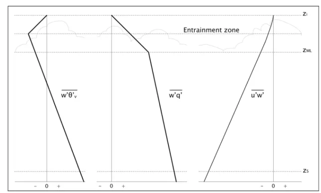
(W m2) In a CBL the mixed layer profiles of vertical fluxes of Θv, q and u are linear (Figure 1.3). The vertical qflux depending on meteorological conditions can decrease or incrase with height. A decrease of Θflux with height to about 0.2 times the surface flux at zi has been commonly observed (LeMone, 2003). In absence ofhorizontal temperature gradients the pressure gradient force is nearly constant with height. Wind components (u) and (v) are nearly constant (Figure 1.2) and hence is possible to derive (Stull, 1997; LeMone, 2003) that the profile of
u'w'
is nearly negatively linear (increasing from negative to zero values at zi)(Figure 1.3).
Fig. 1.3: Idealized vertical profiles of the vertical flux of virtualpotential temperature flux
w'θ'
, specific humidityw'q'
,and the umomentum fluxu'w'
(parallel to the mean surfacelayer wind) (adapted from LeMone 2003).1.2.4. Air quality in CBL
Air pollutants are substances which, when present in the atmosphere under certain conditions, may be injurious to human, animal or microbial life. Two classes of factors determine the amount of pollution at a site (Oke, 1987) (I) the nature of emissions and (II) the state the atmosphere.
laboratory, showed that plume behavior is a function of release height. These results were confirmed by Lamb (1982) and from atmospheric dispersion experiments during the CONDORS field study (Kaimal et al., 1986). Pollutants emitted from smoke stacks exhibit a characteristic looping as those portions of effluent emitted into warm thermals begin to rise and are dispersed rapidly (Figure 1.4). Vertical mixing decrease air pollution near the ground from nearby sources. However, convective conditions can lead high nearsurface concentrations from releases from elevated or distant stacks because the rapid mixing can bring material down to the ground quickly before it has been much diluted, this process is called fumigation (Figure 1.4). Fig. 1.4 Pollutants dispersion on CBL. Looping and Fumigation phenomenons (adapted from Stull 1997). Explicit modelling is needed if one wants to look in detail at the processes that occur in street canyons and to predict canopy level climatology, or to couple detailed traffic emission models with meteorology, in which case knowledge of the vertical profiles of turbulence characteristics in the street canyons is required. Largeeddy simulations is a good tool to study the plume behaviour in the CBL where the large scale turbulent motions are calculated by solving explicitly the equation of motion on a numerical grid and the scales of motion smaller than grid size are parametrized. Largeeddy modelling has been first applied to CBL dispersion by Lamb (1982). When only the overall effect of cities on the overlying ABL is in interest in the context of pollution dispersion at a regional scale, a nonexplicit approach may be sufficient for the main parameters such as albedo, thermal admittance, roughness and moisture availability. In global and mesoscale numerical models, to represent the largest eddies in the CBL who pilots pollutants dispersion, a firstorder gradientdiffusion approach to close the equations with (optionally) a nonlocal or countergradient (Andren 1990, Holtslag and Boville 1993, Hurley 1997) term for scalar fluxes are used. A recently developed alternative method to represent turbulence in the convective boundary layer is one that parameterises the vertical flux of a scalar as the sum of a gradientdiffusion term to represent the smallscale eddies and a massflux term to represent the largescale convective eddies. Siebesma and Teixeira (2000) and Teixeira and Siebesma (2000) used
this approach in the European Centre for MediumRange Weather Forecasts (ECMWF) global model together with a profilespecified eddydiffusivity closure, while Soares et al. (2004) used this approach, together with oneequation prognostic turbulence using the mixing length closure within the mesoNH model. Soares et al. (2004) treated both dry and moist convection in the EddyDiffusivity MassFlux parametrization scheme (EDMF) framework, and demonstrated that this approach has the potential to represent turbulence processes in dry and moist convection within a unified approach rather than as separately parametrised processes. A recent study (Hurley, 2007) applies the EDMF approach but using a twoequation prognostic turbulence equation model within The Air Pollution Model (TAPM; Hurley 2005a, b), combined with the mass flux model from Soares et al. (2004) to modelling mean and turbulence fields in the dry convective boundary layer.
1.3. ABL roles at the “global” and “local” scales
The ABL has an important influence in the behaviour of the atmosphere as a whole. Activities involving the representation of the atmosphere such as climate modelling and numerical weather prediction cannot succeed without the ABL being represented in some detail (Burk, 1989). The main influences on the atmosphere as a whole are as follows: Over level terrain, the drag between the atmosphere and the surface is the main mechanism by which the energy in the largescale motion is dissipated. With smallscale orography the drag also occurs through pressure forces whose magnitude is influenced by the ABL turbulence (Bougeault, 2000). It buffers the transfer of heat and moisture between the surface and the atmosphere, in particular, the way surface solar heating is partitioned into sensible and latent heat fluxes. It is critical in determining the properties of air forming clouds and moist convection. It plays a central role in determining the occurrence of lowlevel clouds and consequential effects on radiation budgets (Siebesma, 1998). It tends to retain aerosols and pollutants from the surface, with the transfer of such polluted air to thefree troposphere being limited mainly to moist convection and frontal motions which, though washout, leave the main atmospheric air freer of such material.
Earth's surface. Prediction and understanding of the local environment requires an understanding of the ABL at the local scale. In particular the ABL is important for predicting a range of parameters such as: the surface wind and turbulence, daily maximum and minimum temperatures, visibility and fog and the dispersion of pollutants and other material.
1.4. Thermal circulations dynamics
Coherent structures tend to be particularly well defined where one type of phenomenon dominates the ABL dynamics (in the case of CBL with low winds, the flotability is the phenomenon who pilots the ABL dynamics). Structures contribute significantly to the overall dynamics of the flow. That is why they tend to determine the form of the velocity spectra, e.g. of the vertical and horizontal components. Structures also affect the statistics of extreme events, such as large gusts or high downbursts of pollution. Coherent structures in the atmosphere need to be understood and described in order to deal more effectively with engineering and environmental problems. Examples are wind energy, wind loading on strucutres, aircraft operation, blowing of dust and snow, propagation of electromagnetic waves, wind shelter design and dispersion of pollution. Study of coherent structures is also helpful in interpreting statistical data (such as spectra, correlations and probability distributions) and can also be used for interpolation when data are not available or for extrapolation to more complex situations. Atmospheric phenomena within the ABL are characterized by space (determined by their typical size or wavelength) and time (typical lifetime or period) scales. Local fluctuations of the circulation derived from differential heating induced by the diurnal cycle and surface heterogeneities belong to the mesoß scale (10100 km) with a typical lifetime of 58 hours (Oke, 1987). Spatial inhomogeneity can originate two diferent effects: Advective effects: horizontal motions starts and air moves from one distinct surface type to a
different one. Thermal circulation system: is the circulation of air induced by contrasting surface properties when regional winds are weak. This last one is our study case, the juxtaposition of contrasting thermal environments resutls in the developement of horizontal pressure gradient forces, which is sufficient to overcome the retarding influence of friction will cause air motion across the boundary between surfaces. Some examples are the Land and sea (lake) beezes, land and water surfaces possess contrasting
thermal responses because of their different properties and energy balance, and this is the driving force behind the land and sea (lake) breeze circulation system encountered near the ocean or lake shorelines. The seabreeze is a well documented mesoscale flow. Studies directed to explore its properties and structure, its dynamics and its overall impact on the air quality of coastal cities from an experimental, numerical or theoretical point of view are numerous. Fisher (1960), Walsh (1974), Atkinson (1981), Rotunno (1983), Nakane (1986), Niino (1987), Finkele (1995), Feliks (1994), Lemonsu (2004c), Lemonsu et al. (2006a, 2006b), Augustin (2006) are only an example of the importance that adquired the field in last decades.
The Urbanbreeze circulation, can develop when regional winds are very light or calm. The horizontal temperature (and therefore pressure) gradient across the urban/rural boundary can be sufficient to induce lowlevel breeze from the country into the city. Urbanbreeze circulation is the central topic of this study and is described in depth in point 3.
2. ABL specificities in urbanized environments
The ABL properties tends to respond to an area average of the surface properties. The accuracy on the description of the surface turbulent flow is a key issue because is critical to the overall ABL properties (Finnigan, 2003). The task of representing the surface is made more difficult by the presence of heterogeneity in the surface as when a city is present.2.1 The urban boundary layer
2.1.1 Definition The Urban Boundary Layer (UBL) is the portion of the ABL above the urban canopy (layer of air between the surface and the roofs level; Oke, 1987) whose climatic characteristics are modified by the presence of a city at the surface. The UBL has received increased attention for characterising and understanding its structure and behaviour (e.g. Oke et al., 1999; Grimmond and Oke 1999a,b). The urban surface morphology and structural characteristics perturbs the ABL and generates atmospheric phenomenons specifics to the urban environment with a characteristic scale going from the microscale to the mesoscale as: reduction of dewfall (Richards, 2004), reduction of radiation fog in within cities (Sachweh and Koepke, 1995; Sachweh and Koepke, 2004), nighttime and daytime heat islands, cold islands, dry islands (described in point 2.2), leeward rainfall enhancement (Sheperd (2005) provides a concise review of recent (1990–present) studiesrelated to how the urban environment affects precipitation), etc.
Comparing with the surrounding landscape the city possesses its own combination of radiative, thermal, moisture and aerodynamic properties, such albedo, soil conductivity, soil moisture, surface roughness, etc. The city tends to regulate and partition the available energy and water (described in section 2.2.3) in a different manner than natural covers (Oke, 1987). Those differences are manifested as different surface, subsurface and atmospheric climates in terms of temperature, humidity and wind speed profiles creating spatial discontinuity and horizontal gradients. Near the surface at the boundaries between the fields these gradients are greatest and horizontal interactions occurs. The climatic response to these spatial variations in surface is further complicated if complicated topography is present. 2.1.2 The urban boundary layer height The UBL, in comparison with the ‘rural’ atmospheric boundary layer (ABL), is characterised by greatly enhanced mixing and Mixing Heights (MH), resulting from both the large surface roughness and increased surface heating. So, the UBL is often considered as a special case of the ABL over a very non homogenous terrain with specific characteristics. The MH is necessary regarding the dispersion of pollution within the canopy and is an important parameter for practically all air pollution applications at the mesoscale and urban scale. Most dispersion models require an estimate of the MH so that any effective limit on vertical spread can be modelled. Its effect is most important when it is shallow, whereby pollutants may be trapped near the ground, leading to high local concentrations, while elevated plumes might be unable to reach the ground. MH estimates may be input to models, or calculated by specific routines within models. Despite progress in numerical turbulent modelling during the last decades, the MH is still one major uncertainty for most air quality models (Piringer et al., 2007). Concerning the methodology of MH determination, fundamental work has been done by COST710 (Seibert et al., 1998). COST715 investigating urban modifications on the MH, both by measurements and parameterisations, and carried out a profound urbanrural intercomparison study for the city of Bologna under different stability conditions (Piringuer and Joffre, 2005). Both from radiosoundings and from numerical modelling there is evidence of increased MH over urban areas compared to their rural surroundings. The urbanrural intercomparison for Bologna resulted in a good internal consistency between the various schemes applied, whilst the sodar cluster of MH values clearly departs from the latter. However, with a careful sodar data analysis, a plausible average daily course of MH can be delineated.
The UBL height is an important parameter for daytime urban heat island generation and urban breeze development as pointed out in Chapters 2, 3 and 4. 2.2 The Urban Heat Island The Urban Heat Island (UHI) is defined as the excess of temperature observed frequently in a metropolitan area in comparison with the surrounding area. Is a wellknown characteristic of the urban micro climate. 2.2.1 Diurnal cycle The UHI has a typical daily cycle: it increases during the late afternoon and reaches its maximum during the night (58ºC for a mediumsize European city; Oke, 1982) decreasing after dawn and generally reaching a minimum value during the morning hours being possible to reach negative values (1ºC, city centre cooler than it surroundings). After that it starts to increase again. The warmth is accumulated reaching 12ºC during daytime (Shea and Auer, 1978; Yoshikado, 1992; Hidalgo et al., 2008a). The causes in the UHI formation are different under nighttime and daytime conditions: During the night, a stable layer of air generally forms in rural areas, due to surface cooling (Oke, 1982). Under calm wind conditions (i.e. conditions favourable to the formation of the UHI), there is no mixing of the air by wind shear and the nocturnal stable layer inversion is strong. This nocturnal inversion can reach a few hundred meters in height. Over a city, however, the SEB is modified and the air is heated by the surface. This reduces the cooling of the atmosphere but is not strong enough to prevent it. However, it is sufficient to maintain mixing with the air above by dry convection. This leads to the development of a neutral or slightly unstable turbulent layer above the city (Figure 1.5). Therefore, during the night, this ambient stability plays a key role in determining both the UHI intensity and the strength of circulation (Scheffler, 1978, 1979; Vukovich and Dunn, 1978; Richardone, 1989).
Fig 1.5: Schematic representation of the potential temperature profiles associated to the urban heat island (a) during the nigth, and (b) during the day. Thin lines are for rural profiles, bold ones for urban profiles. The dashed line in the night case represent the typical structure of the atmosphere above the nocturnal stable layer. During the day, the structure of the lower atmosphere is completely different from its structure at night. In the countryside, the heating of the surface by the sun in the morning produces a heat flux towards the air above that is sufficient, firstly, to destroy the nocturnal stable layer and, secondly, to mix the air (the socalled ‘mixed layer’, Figure 1.5) by turbulence to a much higher altitude (zi), where a capping temperature inversion occurs. This temperature inversion is linked, not to the nocturnal stable layer (which is near the surface), but more to the previous day’s capping inversion (which is still present above the nocturnal inversion, shown by dashed lines on Figure 1.5), to the general meteorological situation and the total heating of the air by the surface during the day. The presence of a city will modify the SEB by heating the atmosphere above it. However, this modification only represents a relatively minor modification of the countryside mixed layer: the UBL will be a little warmer (the daytime UHI), a little more turbulent, and extend slightly higher. Under favourable weather conditions, the daytime UHI can initiate local circulations. 2.2.2 The UHI is modified in function of the meteorological context The UHI effects can be reduced or even disappear under certain regional weather conditions:
demonstrated by Sundborg (1950). Large amounts of clouds blocks the solar incident radiation reducing the diurnal surface heating (Sundborg, 1950). Raining periods also decrease UHI intensity (Yagüe and Zurita, 1991; Runnals and Oke, 2000). Seasons cycle also affects the UHI occurrence frequency (Jauregui, 1997; Kim and Baik, 2002). Numerous studies show the effects of anthropogenic warming on local and regional temperatures in many diverse latitudes. Block et al., (2004) showed effects across central Europe, Zhou et al. (2004) and He et al. (2005) across China, VelazquezLozada et al. (2006) across San Juan, Puerto Rico and Hinkel et al. (2003) even in the village of Barrow, Alaska. In all cases, the warming was greatest at night and in higher latitudes, mainly in winter. 2.2.3 Causes of UHI the generation As population centres grow they tend to modify a greater and greater area of land and have a corresponding increase in average temperature (Oke, 1983). Oke (1973) finds evidence that the UHI (in ̊C) increases according to the formula UHI = 0.73 log10( P ) where P denotes population. The processes conducting to the UHI have been inferred through urban field campaigns focused on the exchanges of energy between the urban surface and the atmosphere (Nuñez and Oke, 1977; Cleugh and Oke, 1986; Oke et al., 1999) and the development of numerical models dedicated to the computation of these exchanges (Arnfield, 1982; Grimmond et al., 1991; Masson, 2000; Martilli et al., 2002). The reason the city is warmer than the country comes down to a difference between the energy gains and losses of each region resulting on a SEB modification. Four common physical characteristics of urban areas modify the SEB and the micrometeorological processes that occur between a surface during the day and the night in comparison with the same the phenomena in a rural area. These four characteristics are:
•
[1] the rarefaction of vegetation and the massive use of impervious materials for buildings and pavements,•
[2] the ability of building materials to store and release large amount of heat within a few hours,•
[3] the threedimensional geometry of the urban surface (urban canyon shape of streets),During the day in rural areas most of the solar energy evaporates water from the vegetation and soil. Thus, while there is a net solar energy gain, this is compensated to some degree by evaporative cooling. In cities, where vegetation is scarce (the property [1] of the urban surface), the buildings, streets and sidewalks absorb the majority of solar energy input and the solar energy is almost completely transformed into heat. Then the property [2] leads to an enhancement of the process of heat storage in the urban materials. As a consequence of these two properties, at the end of the sunlit period, the urban materials have accumulated a higher amount of the solar energy than a typical vegetated rural area. Then, when the night comes, this large stock of energy is released to the air above and delays or reduces the air cooling in the urban canyon. Moreover, the property [3] further limits the cooling rate of the walls and the streets. Each (warm) wall and street of the urban canyon has a reduced skyview factor and sees each other whereas a flat open surface (open to the sky), will cool more rapidly. Finally, the property [4] results in an additional source of heat in urban areas. There are numerous studies analysing and describing UHI features by means of field experiments, numerical approaches and with laboratory models, Pigeon (2007c) made a good review of the UHI stateof art.
2.3. Urban impact on the surface energy balance
Urbanized surface properties modify the SEB (described in section 1.2.3) resulting in atmospheric phenomenon characteristics of urban environments. The urban heat island is one of them. Earlier work in North American cities (Grimmond and Oke, 1999a) motivated that COST715 initiated and conducted several European urban field experiments to investigate whether similar or different perturbations of the surface energy balance partitioning compared to the rural surroundings would occur in European cities. European cities have generally denser urban cores, which should lead to even larger perturbations than reported from the former American studies. The urban SEB may be expressed with directly measured terms (Oke, 1988): Q∗ + Q F = QH + QE + ΔQS + ΔQA Being Q∗ the net allwave radiation flux, QF the anthropogenic/combustion heat flux, QH and QE
aerodynamic turbulent sensible and latent heat fluxes. The term ΔQS is the neat heat flux stored into or
ΔQA =
∫
0 30ρC
pu
∂
T
∂
x
dz
is negligible considering the order of magnitude of the other fluxes. The UHI formed during daytime is the source of the daytime urbanbreeze circulation central topic of this study. The analysis is then centered on this part of the SEB and UHI diurnal cycle and linked to the local circulation (dynamics) generated (an extensive analysis of the complete diurnal cycle is presented in Chapter 2). During daytime in urban areas: The turbulent flux density QH is the primary mean of dissipating the net radiation surplus (due tobuilding materials, 3D geometry and the heat released by the human activities (waste heat generated by energy usage: traffic, space heating or cooling, industry...)) remaining positive even into late evening (after sunset).
As a consequence of use artificial and impervious materials for buildings and pavements, vegetation
is scarce in cities and evotranspiration (QE) is reduced being close to zero in the city center (with no
street cleaning) during summer periods.
Sensible heat storage (ΔQS ) by the system is also a significant term in the balance. The flux
depends on the urban structure, the thermal properties of the urban materials (thermal conductivity, heat capacity), and the sun–surface–atmosphere coupling (Roberts, 2006). During daytime ΔQS is
important to model evaporation, the convective sensible heat flux, and the boundary layer growth (Grimmond et al., 1991; Roth and Oke 1994; Taha, 1997).
Under summer conditions with weak wind, this lower evapotranspiration in the city leads to a preferential channelling of energy into sensible forms (QH and ΔQS ) and therefore a warming of the
environment generating the UHI cited before. To summarize, under daytime conditions the surface heat flux in the countryside can be significant: at least in the morning it is sufficient to build the mixed layer, and most often, it remains positive during the entire day. However the countryside heat flux is lower than the urban one, because of a large consumption of the available solar energy for latent heat flux by the plants. This difference in the heat flux between the city and the countryside is what causes the daytime UHI key feature of the daytime urban breeze circulation. Urban perturbations on the SEB can actually successfully be parameterised. A number of European groups developed detailed urban SEB parameterisations for mesoscale models (Masson 2000; Martilli et al.,
2002; Baklanov et al., 2002; Best, 2005; Dandou et al., 2005, Hamdi and Schayes, 2005; Dupont, 2006; Dupont and Mestayer, 2006). Preliminary studies indicate that the influence of the urban canopy, building energy flows and thermal properties, along with effective albedo reduction by radiative trapping between canyon walls, is important and needs to be properly described in models. These parameterisations will probably become operational in the near future, progress has been made within the EU project FUMAPEX (Baklanov et al., 2006) initiated by COST715. An intercomparison exercise of existing Urban Surface Schemes coordinated from the King's College London, started at the end of 2007. A set of about thirty models is participating in this exercise aimed to evaluate the realism of urban heat exchange, computational performing and paraterizations complexity needed to obtain accurate results (http://www.kcl.ac.uk/ip/suegrimmond/model_comparison.htm).