HAL Id: hal-02912545
https://hal.archives-ouvertes.fr/hal-02912545
Submitted on 29 Jan 2021
HAL is a multi-disciplinary open access archive for the deposit and dissemination of sci-entific research documents, whether they are
pub-L’archive ouverte pluridisciplinaire HAL, est destinée au dépôt et à la diffusion de documents scientifiques de niveau recherche, publiés ou non,
High energy PIXE: A tool to characterize multi-layer
thick samples
A. Subercaze, Charbel Koumeir, Vincent Métivier, Noël Servagent, Arnaud
Guertin, Ferid Haddad
To cite this version:
A. Subercaze, Charbel Koumeir, Vincent Métivier, Noël Servagent, Arnaud Guertin, et al.. High energy PIXE: A tool to characterize multi-layer thick samples. Nuclear Instruments and Methods in Physics Research Section B: Beam Interactions with Materials and Atoms, Elsevier, 2018, 417, pp.41-45. �10.1016/j.nimb.2017.09.009�. �hal-02912545�
High energy PIXE : a tool to characterize multi-layer
thick samples
A. Subercazea, C. Koumeira,b, V. Metiviera, N. Servagenta, A. Guertina, F. Haddada,b
aLaboratoire SUBATECH, Institut Mines T´el´ecom Atlantique, Universit´e de Nantes, CNRS/IN2P3, 4 Rue Alfred Kastler, 44307 Nantes cedex 3 - FRANCE bGIP ARRONAX, 1 rue ARONAX, 44817 Saint-Herblain cedex - FRANCE
Abstract
High energy PIXE is a useful and non-detructive tool to characterize multi-layer thick samples such as cultural heritage objects. In a previous work, we demonstrated the possibility to perform quantitative analysis of simple multi-layer samples using high energy PIXE, without any assumption on their composition. In this work an in-depth study of the parameters involved in the method previously published is proposed. Its extension to more complex samples with a repeated layer is also presented. Experiments have been per-formed at the ARRONAX cyclotron using 68 MeV protons. The thicknesses and sequences of a multi-layer sample including two different layers of the same element have been determined. Performances and limits of this method are presented and discussed.
Keywords: High energy PIXE; Ion beam analysis; Multi-layers; Kα
Kβ ratio.
1. Introduction
Analysis of cultural heritage objects is a very active application field for the PIXE method [1–3], especially thanks to its ability to determine their elemental composition in a non-destructive way. In many cases, those objects consist of a stack of many layers (paintings, coins...) with sometimes several layers made of the same element. Differential PIXE [4], using low ernergy beam, was developped in order to provide depth concentration profile, com-position and ordering of the layers. The principle of this technique relies on the comparison between PIXE spectra recorded at different beam energies
[5] (e.g from 1 to 4 MeV) or at different incident angles [6]. Complementary information about the target is obtained for each measurement due to the strong variation of the ionization cross sections, at low energy, within the target. It is, therefore, possible to use a de-convolution algorithm to extract the contribution of each layer. Differential PIXE has been used to study multi-layer samples [7] with a thickness up to tens of microns [8].
High-energy PIXE (HEPIXE) is suitable to perform non destructive anal-ysis of thick samples, in normal air, due to the high penetration range of energetic light ions in matter and their ability to excite the energetic K X-rays. HEPIXE has already been used in the field of cultural heritage [9–11] and especially for the characterization of ancient paintings with several su-perposed layers [12]. Metallic archeological objects can be also investigated without removing the patina layer present on their surface. The investi-gated thicknesses in those works were between few dozens and few hundred of micrometers. But in this case, contrary to the usual differential PIXE method, ionization cross sections change smoothly with the energy and inci-dent angle variation. However, HEPIXE analysis using Kα
Kβ (or
Kα
Lα,
Lα
Lβ) ratio
provides qualitative information about the thicknesses and the sequences of several layers but assumptions on the sample composition is required [12]. In a recent work [13], we demonstrate the possibility to perform quantita-tive analysis of simple multi-layer samples without any assumption on their composition. This method, based on the relative variation of Kα
Kβ (or
Kα
Lα,
Lβ
Kα)
when the sample is rotated, had given good results for patterns of different pure material foils. But in more realistic applications, there might be some repetition of a layer inside the samples. The present work aims at studying samples with repeteated layers based also on the relative variation of Kα
Kβ (or
Kα
Lα,
Lβ
Kα) ratio. This study is an extention of the previous method [13] and
it is a step further to develop an acurate quantitative method in order to analyze cultural heritage samples later on. Firstly the experimental setup is described. Secondly, the key parameters of the method such as the self at-tenuation and the impact of the layer placed in front of the emitting one are described. Finally, the extension of the previous method [13] to the analysis of a multi-layer sample with a repeated layer is presented.
2. Experimental procedure 2.1. Experimental set-up
High energy experiments were carried out at ARRONAX cyclotron [14] using 68 MeV protons. The beam diameter on the sample was in the range of 1 cm. The X-rays are detected by a High Purity Germanium (HPGe) detector. The distance between the sample and the detector is 25 cm. The sample holder can be rotated with respect to the incident beam in order to change the angle between the sample and the detector, with a precision of 0.01◦. An ionization chamber is used in order to monitor the number of par-ticles penetrating the samples. The ionization chamber current is measured by a high precision commercial electrometer (MULTIDOS-PTW). Prior to the samples irradiations, the ionization chamber is calibrated using a faraday cup. During the experiments, the beam intensity is kept around 100 pA and the irradiations last about 15 minutes. The high energy PIXE platform is described in more details in [15].
2.2. Studied samples
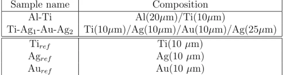
The composition and the thickness of the samples prepared for this work are listed in table 1. The samples are composed by a stack of several pure material foils. Those foils are provided by GoodFellow and their dimensions are 25x25 mm2. The Al-Ti sample is used to study the linearity of ∆µ · d (see section 3.2) involved in the determination of the layers thicknesses. The Ti-Ag1-Au-Ag2 is prepared as a multi-layer sample with a repeated layer in order to perform the associated analysis. References samples for each elements are also irradiated using the same experimental configuration as the Ti-Ag1-Au-Ag2 irradiation. Those reference samples are used to reduce the experimental errors (such as detection efficiency) on the quantification of the layers thicknesses.
Table 1: Composition of the irradiated samples for this study. The value in the parenthesis is the thickness of the given pure foil.
Sample name Composition Al-Ti Al(20µm)/Ti(10µm)
Ti-Ag1-Au-Ag2 Ti(10µm)/Ag(10µm)/Au(10µm)/Ag(25µm)
Tiref Ti(10 µm)
Agref Ag(10 µm)
The thicknesses of the foils presented in table 1 are given by GoodFellow. Acurate values obtained using a scanned and a high precision scale for the Ti of Ti-Ag1-Au-Ag2 are presented in table 4.
2.3. Multi-layer analysis method
The analysis method [13] is based on the relative variation of Kα
Kβ (or
Kα
Lα,
Lβ
Kα) ratio (Kαis the number of detected KαX-rays), named
∆R
R , as a function of the angle between the target and the detector, θ = 0 when the detector axis is normal to the sample, i.e their surfaces are parallel. This relative variation is given by : ∆R R = R(θ1) − R(θ2) R(θ1) = 1 − fself · e( ∆µ·dcos(θ 2)) e( ∆µ·d cos(θ1)) , (1)
where ∆µ = µKβ − µKα with µ the attenuation coefficient [16] of the
layers placed in front of the emitting one, d is X-rays path in this layer and fself is given by the equation :
fself = 1−e (−µ 0 α·d 0 cos(θ2)) 1−e( −µ0 β·d 0 cos(θ2)) 1−e (−µ 0 α·d0 cos(θ1)) 1−e( −µ0 β·d 0 cos(θ1)) , (2)
where µ0 is the attenuation coefficient of the emitting layer and d0 the X-rays path inside it. The function fself represents the ratio of the Kα
Kβ attenuation
in the emitter layer itself, in other words the self attenuation. The impact of this factor is presented in the next section.
When fself is negligible, we can extract from equation 1 :
∆µ · d = 1 1 cos(θ2) − 1 cos(θ1) · ln(1 −∆R R ). (3)
∆µ · d contains the attenuation of the effective layer located between the emitting one and the detector (the effective layer has the same effect on the X-ray attenuation than real layers). Using the photoelectric mass attenuation
coefficient (far from the shell edge), µρ given in [17] and equation 3 we can calculate the attenuation of Kα lines (or Kβ, Lα, Lβ) MKα
MKα = n X i=0 e(−µiα·di) = e −∆µ·d· 1 (EKα )7/2 1 (EKβ)7/2 − 1 (EKα )7/2 , (4)
where n is the number of layers placed in front of the emitting one and E the energy of the considered X-ray. The detected number of Kα X-rays (or Kβ, Lα, Lβ), NKlayerα , can then be corrected from this attenuation . Therefore we
can determine the thickness of a layer, elayer
elayer = − 1 µ0α · ln 1 − NKlayerα NStandard Kα · MKα ! , (5)
where NKStandardα is the X-ray intensity of a standard sample irradiated in the same condition.
To determine the sequence of a multi-layer sample, ∆µ · d can’t be used because of its dependency on the energy of the X-rays. Using the definition of µρ given in [17], we can calculate a new term (∆µ · d)0 defined by equation 6. (∆µ · d)0 = 1 1 E7/2Kβ − 1 EKα7/2 · 1 1 cos(θ2) − 1 cos(θ1) · ln(1 −∆R R ) (6) (∆µ·d)0 is also equal to : ρ·d·Z5·Na
A, where E is the energy of the considered X-ray, NA is the Avogadro constant and Z, A, ρ, d are the effective atomic number, mass number, density and thickness of the layers placed in front of the emitting one. The comparison between (∆µ · d)0 values for each detected elements allows to determine the sequences of the layers (demonstrated in [13]).
3. Robustness of the method
In this section, the main parameters (described in the previous section) of the analysis method are studied.
3.1. Self attenuation
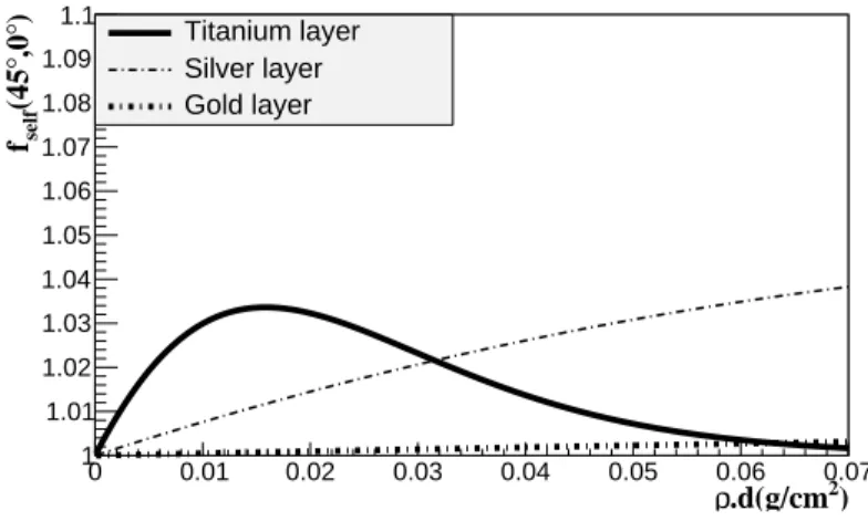
The relative variation of R, ∆RR , is function of the self attenuation and of the attenuation inside the layers placed above the emitting one. In order to use ∆RR to determine the thickness and the position of the emitting layer, the self attenuation factor has to be small compared to the attenuation inside the layers. The variation of the self attenuation factor, fself, as a function of the emitting layer thickness (g.cm−2) and for θ1 = 45◦ and θ2 = 0◦ is shown in figure 1. These angles have been choosen because they lead to the maximum variation of the self attenuation factor (i.e the worst case).
) 2 .d(g/cm ρ 0 0.01 0.02 0.03 0.04 0.05 0.06 0.07 ) ° ,0 ° (45 self f 1 1.01 1.02 1.03 1.04 1.05 1.06 1.07 1.08 1.09 1.1 Titanium layer Silver layer Gold layer
Figure 1: fself as a function of ρ · d calculated using equation 2 for titanium, silver and gold and for θ1 = 45◦ and θ2 = 0◦. The self attenuation factor is calculated for the KKαβ ratio.
For these three elements (Ti, Ag and Au representing a wide range of Z), the self attenuation factor is less than 1.04.
For the titanium, due to its low energy X-ray, even a low amount of light element in front of it will induce a value of ∆RR far larger than 1.04. For example, 20 µm of aluminium gives ∆RR =1.15 for the titanium. So the self attenuation is negligeable and is not an issue for light element.
In the silver case, a low value of ∆RR (1-3%) can be due to the self attenu-ation of a thick Ag layer or to the attenuattenu-ation by the layers above in case of a thin Ag layer. We can solve this issue using the value of the Kα intensity. In fact a thick layer of Ag will induce a higher Kα intensity compared to a thin one.
In the gold case, the self attenuation factor is lower than 1.01, but in the majority of the cases the Kα
Kβ ratio will not vary so much due to the high
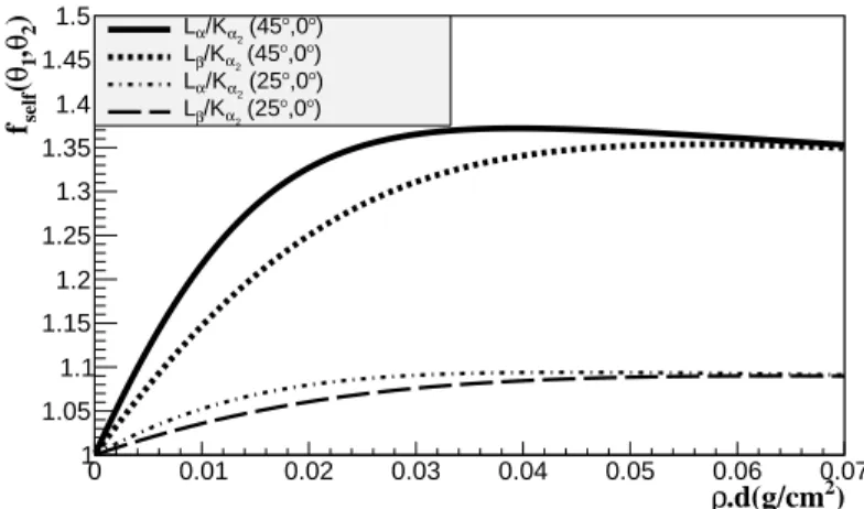
energy K X-rays. Therefore this ratio cannot be used (or in very specific cases like very thick samples). Lα
Kα or
Lβ
Kα ratios can be used instead. The variation
of fself in this case is represented in figure 2. For the couple of angles (45◦, 0◦), the self attenuation factor is too high (up to 1.35) but by choosing a smaller angle variation (25◦) we can reduce fself. Due to the low energy of the L X-rays, even for a narrowed angular range, the angular variations of those ratio are sensitive to thin layer (few dozens of µm) contrary to the Kα
Kβ
ratio. Therefore for heavy elements we can use the Lα
Kα (or
Lβ
Kα) ratio and a
narrowed angular range to determine the sequences and the thicknesses with a negligible influence of the self attenuation.
) 2 .d(g/cm ρ 0 0.01 0.02 0.03 0.04 0.05 0.06 0.07 )2 θ ,1 θ ( self f 1 1.05 1.1 1.15 1.2 1.25 1.3 1.35 1.4 1.45 1.5 (45°,0°) 2 α /K α L ) ° ,0 ° (45 2 α /K β L ) ° ,0 ° (25 2 α /K α L ) ° ,0 ° (25 2 α /K β L
Figure 2: Self attenuation factor as a function ρ · d calculated using equation 2 for the gold and for θ1= 45 or 25◦ and θ2= 0◦. The self attenuation factor is calculated for the Lα
Kα
and Lβ
Kα ratio.
Looking at the self attenuation factor for different elements, we have defined a framework for the method. Analysis of light elements is not affected by the self attenuation. For mid-Z elements and low value of ∆RR , the value of the Kα intensity has to be considered. For heavy elements, the ratio
Lα,β
Kα
has to be used instead of the Kα
Kβ with a lower angles (θ2- θ1).
3.2. Attenuation in layers placed in front of the emetting layer :∆µ · d The normalization of ∆µ · d by cos(θ1
2)−
1
cos(θ1) remove the angular
The Sample Al(20 µm)/Ti(10 µm) is irradiated in order to compare the value of ∆µ · d with those previously obtained with a Al(50 µm)/Ti(10 µm) sample [13]. The mean value of ∆µ · d (calculated with 3 different couples of angles θ1, θ2) for 20 µm aluminium is equal to -0.35 ± 0.03, whereas the mean value was equal to -0.90 ± 0.06 for the thicker sample in [13]. The ratio of this two values, 2.57 ± 0.09, is equal to the ratio of the aluminium thicknessses which is equal to 2.5 (50/20). Therefore, results show a linear behavior of ∆µ · d with the attenuation layer thickness.
If the emitting element is repeated in several separated layers, equation 3 is no longer valid, and the calculated ∆µ · d will vary with the choice of θ1 and θ2. Therefore it’s a way to determine if an element is repeated or not. For this purpose a minimum of 3 irradiations with 3 different detection angles are required to check the variation of ∆µ · d.
4. Analysis of a multi-layer sample with two layers of the same element
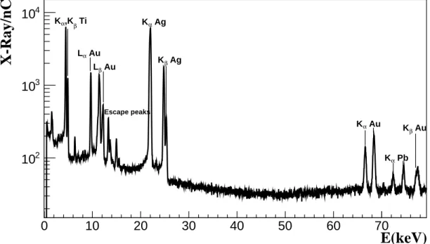
A sample have been irradiated with a 68 MeV proton beam with three different detection angles. Fig 3 shows one of the obtained spectra. Three el-ements (titanium, silver and gold) are detected thanks to their characteristic X-rays.
E(keV)
0 10 20 30 40 50 60 70X-Ray/nC
2 10 3 10 4 10 Ti β ,K α K Au α L Au β L Escape peaks Ag α K Ag β K Au α K Pb α K Au β KFigure 3: Spectra of the investigated target obtained using 68 MeV proton beam with the detector normal to the target surface (θ= 0◦).
For the titanium, the ratio of the Kα
Kβ intensity is constant when θ varies
(see table 2). We can then, deduce that there is no layer in front of the tita-nium, and its thickness is determined (see table 4) using equation 5 without the attenuation correction.
Table 2: Values of R for the titanium as a function of θ.
θ(◦) R 0 5.43 ± 0.22 22 5.43 ± 0.22 45 5.42 ± 0.22
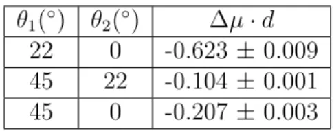
In the gold case, R (calculated using Lα and Kα lines) varies with the detec-tion angle so equadetec-tion 5 is used to determine its thickness (see table 4). For the silver, in contrary to the others layers, ∆µ · d is not constant with θ (see table 3).
θ1(◦) θ2(◦) ∆µ · d 22 0 -0.623 ± 0.009 45 22 -0.104 ± 0.001 45 0 -0.207 ± 0.003
This variation signs more than one silver layer inside the sample. All those information (three elements detected in the spectrum, the titanium is the first layer and the silver is the only element to be repeated) give us the sequences of the layers (see figure 4).
Figure 4: Scheme of the layers sequences inside the irradiated target.
Therefore the following sequence is the only one possible : titanium is the first layer, the second and the last are made of silver and gold is the third layer.
Therefore the attenuation, AAu, of the X-ray from the gold layer is the product of the attenuation by the titanium and the first layer of silver and is given by :
AAu = e−µT i·dT i· e−µAg1·dAg1 (7)
Equation 4 is used to calculate AAufrom the value of ∆µ·d. We can calculate the thickness ( see table 4) of the first layer of silver using :
dAg1 =
−1 µAg · ln(
AAu
e−µT i·dT i). (8)
In the spectra, the intensity of the silver X-ray is the sum of the con-tribution from the two layers. Knowing the thickness of the first layer, we can calculate its X-ray intensity and therefore determine the intensity of the second layer IAg2. This intensity, IAg2, is then corrected by the
attenua-tion of the other layers (titanium, silver, gold) to determine the second layer thickness by using the same method as for titanium (see table 4).
Element Calculated thickness(µm) Real thickness(µm) Titanium 10.13 ± 1.23 10.3 ± 0.02 Silver (1) 9.23 ± 0.91 10.4 ± 0.02 Gold 9.8 ± 1.08 10.79 ± 0.02 Silver (2) 23.3 ± 2.4 24.59 ± 0.01
The calculated thicknesses presented in table 4 are in good agreement with the real thicknesses of each layers of our samples, even for the repeated layer.
Some limitations to be worked out :
We were able to determine the thickness of the second silver layer with a small relative error, because its contribution to the total X-ray intensity is significant. In the case of a non repeated layer, using ∆µ · d to determine the thickness of each layer [13], the error doesn’t depend of the number of layers. To calculate the thickness of the repeated layers, the thickness of each layer in front of the considered ones is required. The uncertainty calculated using the propagation uncertainty formula will increase with the number of layers in front of the repeated one. The performance of this method in those cases depends on the studied object (number of layers, sequences, thicknesses of the repeated layers).
In more complex cases, with multiple repetition, this method is no longer applicable. But the use at the same time of complementary IBA techniques, such as PIGE or detection of charged particles, could provides additionnal useful information to deal with those more complex cases.
5. Conclusion
We demonstrate the possibility to perform quantitative analysis of multi-layer targets using high energy PIXE, without any assumption on their com-position. A proper study of the parameters involved in the method previ-ously published [13] is presented and more complex cases are investigated. The framework of the method depending on the atomic number of the ana-lyzed element has been defined by looking at the self attenuation factor. We demonstrate the linearity of ∆µ · d involved in the thickness calculation.
An extension of this analysis method also based on the relative variation of Kα
Kβ (or
Kα
Lα,
Lα
Lβ) when the sample is rotated, has been applied to a
layers without assumption on the sample composition have been determined even for the repeated layer. For samples without any repeated layer, the error on the thickness is low. In the case of a repeated layer, the X-ray intensity has to be significant to apply this method.
The thicknesses determined in this work are in the same order of magni-tude as in cultural heritage samples analysed by PIXE. The performance of this method will be tested on real cases and especially on art objects already analysed by HEPIXE in the near future.
Acknowledgments
The ARRONAX cyclotron is a project promoted by the Regional Council of Pays de la Loire financed by local authorities, the French government and the European Union. This work has been, in part, supported by a grant from the French National Agency for Research called Investissements dAvenir, Equipex Arronax-Plus no ANR-11-EQPX-0004.
Reference
[1] R. Borges, L. Alves, R. Silva, M. Ara´ujo, A. Candeias, V. Corregidor, P. Val´erio, P. Barrulas, Investigation of surface silver enrichment in an-cient high silver alloys by PIXE, EDXRF, LA-ICP-MS and SEM-EDS, Microchemical Journal 131 (2017) 103–111.
[2] A. Zucchiatti, A. C. Font, P. C. G. Neira, A. Perea, P. F. Esquivel, S. R. Llorens, J. L. R. Sil, A. Verde, Prehispanic goldwork technology study by PIXE analysis, Nuclear Instruments and Methods in Physics Research Section B: Beam Interactions with Materials and Atoms 332 (2014) 160–164.
[3] M. Rizzutto, M. Moro, T. Silva, G. Trindade, N. Added, M. Tabacniks, E. Kajiya, P. Campos, A. Magalh˜aes, M. Barbosa, External-PIXE anal-ysis for the study of pigments from a painting from the Museum of Con-temporary Art, Nuclear Instruments and Methods in Physics Research Section B: Beam Interactions with Materials and Atoms 332 (2014) 411– 414.
[4] P. Midy, I. Brissaud, Application of a new algorithm to depth profiling by PIXE, Nuclear Instruments and Methods in Physics Research Section
[5] I. Brissaud, G. Lagarde, P. Midy, Study of multilayers by PIXE tech-nique. Application to paintings, Nuclear Instruments and Methods in Physics Research Section B: Beam Interactions with Materials and Atoms 117 (1-2) (1996) 179–185.
[6] G. Weber, D. Strivay, L. Martinot, H.-P. Garnir, Use of PIXE–PIGE under variable incident angle for ancient glass corrosion measurements, Nuclear Instruments and Methods in Physics Research Section B: Beam Interactions with Materials and Atoms 189 (1) (2002) 350–357.
[7] ˇZ. ˇSmit, J. Isteniˇc, T. Knific, Plating of archaeological metallic objects– studies by differential PIXE, Nuclear Instruments and Methods in Physics Research Section B: Beam Interactions with Materials and Atoms 266 (10) (2008) 2329–2333.
[8] P. Mand`o, M. Fedi, N. Grassi, A. Migliori, Differential PIXE for in-vestigating the layer structure of paintings, Nuclear Instruments and Methods in Physics Research Section B: Beam Interactions with Mate-rials and Atoms 239 (1) (2005) 71–76.
[9] A. Denker, K. Maier, Investigation of objects d’art by PIXE with 68 MeV protons, Nuclear Instruments and Methods in Physics Research Section B: Beam Interactions with Materials and Atoms 161 (2000) 704– 708.
[10] A. Denker, M. Blaich, PIXE analysis of Middle Age objects using 68 MeV protons, Nuclear Instruments and Methods in Physics Research Section B: Beam Interactions with Materials and Atoms 189 (1) (2002) 315–319.
[11] T. Dupuis, G. Chene, F. Mathis, A. Marchal, M. Philippe, H.-P. Gar-nir, D. Strivay, Preliminary experiments: High-energy alpha PIXE in archaeometry, Nuclear Instruments and Methods in Physics Research Section B: Beam Interactions with Materials and Atoms 268 (11) (2010) 1911–1915.
[12] A. Denker, J. Opitz-Coutureau, Paintings–high-energy protons detect pigments and paint-layers, Nuclear Instruments and Methods in Physics Research Section B: Beam Interactions with Materials and Atoms 213 (2004) 677–682.
[13] A. Subercaze, A. Guertin, F. Haddad, C. Koumeir, V. M´etivier, N. Ser-vagent, Thick multi-layers analysis using high energy PIXE, Nuclear Instruments and Methods in Physics Research Section B: Beam Inter-actions with Materials and Atoms.
[14] F. Haddad, L. Ferrer, A. Guertin, T. Carlier, N. Michel, J. Barbet, J.-F. Chatal, ARRONAX, a high-energy and high-intensity cyclotron for nuclear medicine, European Journal of Nuclear Medicine and Molecular Imaging 35 (7) (2008) 1377–1387.
[15] D. Ragheb, C. Koumeir, V. M´etivier, J. Gaudillot, A. Guertin, F. Had-dad, N. Michel, N. Servagent, Development of a PIXE method at high energy with the ARRONAX cyclotron, Journal of Radioanalytical and Nuclear Chemistry 302 (2) (2014) 895–901.
[16] P. Linstrom, W. Mallard, National Institute of Standards and Technol-ogy: Gaithersburg, MD, March 20899.
[17] W. Heitler, The quantum theory of radiation, Courier Corporation, 1954.
[18] I. Orli´c, I. Bogdanovi´c, S. Zhou, J. Sanchez, Parametrization of the total photon mass attenuation coefficients for photon energies between 100 eV and 1000 MeV, Nuclear Instruments and Methods in Physics Research Section B: Beam Interactions with Materials and Atoms 150 (1) (1999) 40–45.