Université de Montréal
Designing Regularizers and Architectures for Recurrent Neural Networks
par David Krueger
Département d’informatique et de recherche opérationnelle Faculté des arts et des sciences
Mémoire présenté à la Faculté des études supérieures en vue de l’obtention du grade de Maître ès sciences (M.Sc.)
en informatique
Janvier, 2016
c
RÉSUMÉ
Cette thèse contribue a la recherche vers l’intelligence artificielle en utilisant des méthodes connexionnistes. Les réseaux de neurones récurrents sont un ensemble de modèles séquentiels de plus en plus populaires capable en principe d’apprendre des al-gorithmes arbitraires. Ces modèles effectuent un apprentissage en profondeur, un type d’apprentissage machine. Sa généralité et son succès empirique en font un sujet intéres-sant pour la recherche et un outil prometteur pour la création de l’intelligence artificielle plus générale.
Le premier chapitre de cette thèse donne un bref aperçu des sujets de fonds: l’intelligence artificielle, l’apprentissage machine, l’apprentissage en profondeur et les réseaux de neu-rones récurrents. Les trois chapitres suivants couvrent ces sujets de manière de plus en plus spécifiques. Enfin, nous présentons quelques contributions apportées aux réseaux de neurones récurrents.
Le chapitre 5 présente nos travaux de régularisation des réseaux de neurones récur-rents. La régularisation vise à améliorer la capacité de généralisation du modèle, et joue un role clé dans la performance de plusieurs applications des réseaux de neurones récur-rents, en particulier en reconnaissance vocale. Notre approche donne l’état de l’art sur TIMIT, un benchmark standard pour cette tâche.
Le chapitre 6 présente une seconde ligne de travail, toujours en cours, qui explore une nouvelle architecture pour les réseaux de neurones récurrents. Les réseaux de neu-rones récurrents maintiennent un état caché qui représente leurs observations antérieures. L’idée de ce travail est de coder certaines dynamiques abstraites dans l’état caché, don-nant au réseau une manière naturelle d’encoder des tendances cohérentes de l’état de son environnement. Notre travail est fondé sur un modèle existant; nous décrivons ce travail et nos contributions avec notamment une expérience préliminaire.
Mots clés: réseau de neurones, apprentissage machine, apprentissage profond, régularisation, intelligence artificielle, apprentissage supervisé, apprentissage non supervisé, reconnaissance vocale, modélisation du langage
ABSTRACT
This thesis represents incremental work towards artificial intelligence using connec-tionist methods. Recurrent neural networks are a set of increasingly popular sequential models capable in principle of learning arbitrary algorithms. These models perform deep learning, a type of machine learning. Their generality and empirical success makes them an attractive candidate for further work and a promising tool for creating more general artificial intelligence.
The first chapter of this thesis gives a brief overview of the background topics: arti-ficial intelligence, machine learning, deep learning, and recurrent neural nets. The next three chapters cover these topics in order of increasing specificity. Finally, we contribute some general methods for recurrent neural networks.
Chapter 5 presents our work on the topic of recurrent neural network regularization. Regularization aims to improve a model’s generalization ability, and is a key bottleneck in the performance for several applications of recurrent neural networks, most notably speech recognition. Our approach gives state of the art results on the standard TIMIT benchmark for this task.
Chapter 6 presents the second line of work, still in progress, exploring a new ar-chitecture for recurrent neural nets. Recurrent neural networks maintain a hidden state which represents their previous observations. The idea of this work is to encode some abstract dynamics in the hidden state, giving the network a natural way to encode con-sistent or slow-changing trends in the state of its environment. Our work builds on a previously developed model; we describe this previous work and our contributions, in-cluding a preliminary experiment.
Keywords: neural networks, machine learning, deep learning, regularization, artificial intelligence, supervised learning, unsupervised learning, speech recogni-tion, language modeling.
CONTENTS
RÉSUMÉ . . . ii
ABSTRACT . . . iii
CONTENTS . . . iv
LIST OF TABLES . . . vii
LIST OF FIGURES . . . viii
LIST OF ABBREVIATIONS . . . ix
ACKNOWLEDGMENTS . . . xi
CHAPTER 1: INTRODUCTION . . . 1
1.1 Artificial Intelligence (AI) . . . 2
1.2 Machine Learning (ML) . . . 3
1.3 Deep Learning (DL) . . . 3
1.4 Recurrent Neural Networks (RNNs) . . . 5
CHAPTER 2: MACHINE LEARNING . . . 6
2.1 A simple example . . . 6
2.2 What is machine learning? . . . 8
2.2.1 The data generating process . . . 8
2.2.2 Parametric and nonparametric ML . . . 9
2.2.3 Supervised and unsupervised learning . . . 10
2.2.4 Generative models . . . 11
2.2.5 Cost functions . . . 11
2.2.6 Types of SL: classification, regression, and structured output . . 13
2.3 Optimization (minimizing cost) . . . 16
2.4 Generalization, overfitting and regularization . . . 18
2.4.1 Early stopping . . . 19
2.4.2 Regularization . . . 19
2.4.3 Occam’s razor and model complexity . . . 20
2.4.4 Risk minimization . . . 22
2.4.5 Bias and variance . . . 22
2.5 The ML research process . . . 23
CHAPTER 3: DEEP LEARNING AND REPRESENTATION LEARNING 25 3.1 Artificial neural networks . . . 25
3.1.1 Biological inspirations and analogies . . . 25
3.1.2 Neural net basics . . . 26
3.1.3 Activation functions . . . 28
3.2 Features and representations . . . 30
3.2.1 Deep learning and representation learning . . . 32
3.3 Some important deep learning techniques . . . 34
3.3.1 Faster computers . . . 35
3.3.2 Optimization techniques: stochastic gradient descent, momen-tum, RMSProp, Adam . . . 35
3.3.3 Deep learning regularization: dropout and batch normalization . 37 CHAPTER 4: RECURRENT NEURAL NETWORKS . . . 39
4.1 Recurrent neural network architectures . . . 41
4.1.1 Simple RNNs . . . 41
4.1.2 Long short-term memory . . . 41
4.1.3 Gated recurrent units . . . 42
4.1.4 Deep RNNs . . . 42
4.1.5 Attention modules . . . 43
4.1.6 Memory interfaces . . . 43
4.2 Regularization for recurrent neural networks . . . 44
CHAPTER 5: REGULARIZING RNNS BY STABILIZING ACTIVATIONS 45 5.1 Prologue to the paper . . . 45
5.2 Abstract . . . 46
5.3 Introduction . . . 46
5.4 Experiments . . . 48
5.4.1 Character-level language modelling on PennTreebank . . . 48
5.4.2 Phoneme recognition on TIMIT . . . 50
5.4.3 Adding task . . . 52
5.4.4 Visualizing the effects of norm-stabilization . . . 53
5.5 Conclusion . . . 56
CHAPTER 6: CONDITIONAL PREDICTIVE GATING PYRAMIDS . . 57
6.1 Predictive gating pyramids . . . 57
6.1.1 Gated autoencoders . . . 57
6.1.2 Predictive gating pyramids . . . 58
6.2 Conditional predictive gating pyramids . . . 59
6.3 Future work . . . 60
CHAPTER 7: CONCLUSION . . . 62
LIST OF TABLES
2.I Different ways of defining supervised vs. unsupervised learning. . 10 2.II Encoding categories as mathematical objects . . . 14 5.I LSTM Performance (bits-per-character) on PennTreebank for
dif-ferent values of β . . . 49 5.II Performance with and without norm-stabilizer penalty for
differ-ent activation functions. . . 50 5.III Performance (bits-per-character) of zero-bias IRNN with various
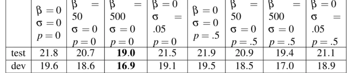
penalty terms designed to encourage norm stability. . . 50 5.IV Phoneme Error Rate (PER) on TIMIT for different experiment
set-tings . . . 52 5.V Phoneme Error Rate (PER) on TIMIT for experiments with more
LIST OF FIGURES
2.1 Overfitting and Underfitting with polynomial regression . . . 19
3.1 The computation performed by a single neuron in a neural network. 26 3.2 An MLP with two hidden layers. . . 27
3.3 Neural net activation functions . . . 28
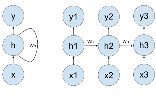
4.1 Unrolling a recurrent neural network. . . 40
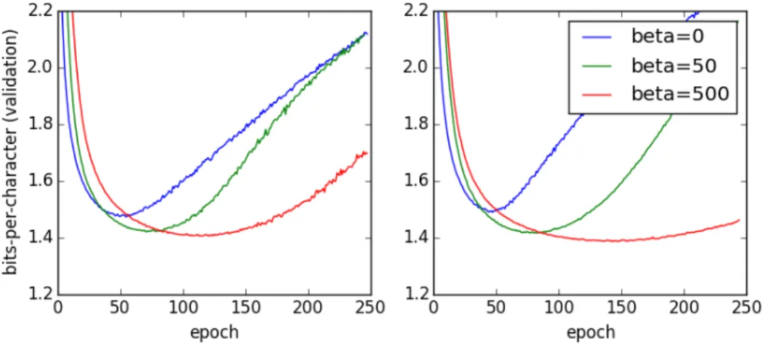
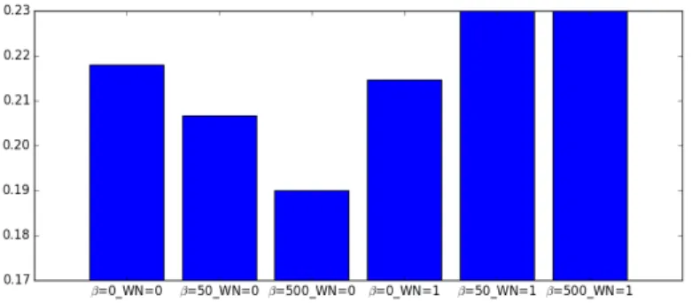
5.1 Learning Curves for LSTM with different values of β . . . 49
5.2 Average PER on TIMIT core test set for different combinations or regularizers. . . 51
5.3 Norm of LSTM hidden states and memory cells for different val-ues of β across time-steps. . . 53
5.4 Average log-norm of hiddens and average cost, as a function of time-step . . . 55
5.5 Hidden norms for values from 0 to 400 of the norm-stabilizer vs. a penalty on the initial and final norms . . . 55
5.6 Average forget gates (LSTM) and eigenvalues (IRNN) with and without norm-stabilizer. . . 55
6.1 Conditional predictive gating pyramid trained on sine waves with frequencies modulated by a random walk . . . 60
LIST OF ABBREVIATIONS
AE Autoencoder
AGI Artificial General Intelligence AI Artificial Intelligence
ANN Artificial Neural Network
BLEU Bilingual Evaluation Understudy BN Batch Normalization
CAD Computer Aided Design
CPGP Conditional Predictive Gating Pyramid CTC Connectionist Temporal Classification
DL Deep Learning
DNN Deep Neural Network
FAI Friendly Artificial Intelligence FGAE Factored Gated Autoencoder
FNN Feedforward Neural Network GAE Gated Autoencoder
Graphics Processing Unit
GRU Gated Recurrent Unit
IRNN Identity Recurrent Neural Network IRL Inverse Reinforcement Learning LSTM Long Short-Term Memory
LM Language Model ML Machine Learning
MLP Multi-Layer Perceptron MSE Mean Squared Error
NaN Not a Number
NLP Natural Language Processing NTM Neural Turing Machine
PGP Predictive Gating Pyramid RL Reinforcement Learning ReLU Rectified Linear Unit
RNN Recurrent Neural Network SGD Stochastic Gradient Descent
SL Supervised Learning
SRNN Simple Recurrent Neural Network SVM Support Vector Machine
TRec Threshold Rectified Linear Unit UL Unsupervised Learning
ACKNOWLEDGMENTS
I would like to thank everyone who helped me onto the path that lead me to complete this thesis, as well as those who made the journey more interesting, enjoyable, and/or manageable. In reverse chronological order, I gratefully thank: My sister Gretchen for proofreading. Alexandre de Brébisson for a great deal of help with the French text of the Résumé. Celine Begin for helping me navigate the administrative procedures of the university and the thesis process. My supervisors Yoshua Bengio and Roland Memisevic for creating a collaborative and open research atmosphere in the lab and for funding my studies and giving me the freedom to pursue interesting topics. Roland in particular for frequent impromptu discussions and guidance on how to make things actually work. Many amazing members of the LISA/MILA lab, including professors, visitors, and staff, for many fascinating and/or entertaining discussions, and invaluable help, advice, encouragement, and good times. The members of the RLLAB at McGill for the same and for welcoming me to their lab for talks and reading groups, or just to hang out and talk. The entire AI safety community for their work on this critical problem, and for helping bring existential risk into mainstream discourse in the machine learning community and society at large. Jelena Luketina in particular for inviting me to the 2015 CFAR reunion. All of my coauthors for the chance to work with and learn from them. Laurent Dinh in particular for patiently teaching me quite a bit about machine learning in the earlier stages of my degree. Daphne Koller and Andrew Ng for creating Coursera, and Geoff Hinton for his Coursera course, without which I almost certainly would not have heard about the phenomenon of Deep Learning in time to start this program when I did. My Freshman year housing advisor at Reed, Hassan Ghani, for inspiring me to seriously consider the possibility that artificial intelligence could be developed and the ethical significance of such an occurrence. All of the wonderful teachers I’ve had over the years who inspired me to keep studying. Finally, my family and friends for everything they’ve done for me over the years.
CHAPTER 1
INTRODUCTION
The subject matter of this thesis is artificial intelligence (AI), specifically machine learning (ML). More specifically, I focus on deep learning (DL) and in particular recur-rent neural networks (RNNs). I’ll introduce these topics briefly before delving into more detail in the following chapters, which provide the necessary background for the rest of the thesis, as well as a brief overview of these topics.
I’ll attempt to describe the current state of AI, ML, DL, and RNN research, and how they relate to one another, making an effort to be informative as to current practices and recent trends. My goal is to give a glimpse of the world of artificial intelligence from the perspective of a deep learning researcher at the beginning of 2016, a time when artificial intelligence and deep learning are making headlines and capturing people’s attention and imagination to an unprecedented extent. As such, broad statements about trends in these fields should be taken as my personal impressions which I feel confident enough to state as such. I hope that some degree of subjectivity can be accepted as a price for this insider’s perspective, since I imagine it could be both interesting and informative to someone unfamiliar with the field.
I mostly use the “companionate we” for the rest of the thesis, occasionally slipping back into first-person singular for opinionative remarks. We assume some familiarity with calculus, linear algebra, probability, statistics, computer science, and graph theory. We attempt to be quite general in our definitions, but some of our terminology may be used in a more (or less) restrictive way in practice, depending on context.
1.1 Artificial Intelligence (AI)
We define artificial intelligence as the study of intelligent behaviour 1. We distin-guish narrow AI from artificial general intelligence (AGI). Narrow AI is about solving specific tasks which are considered indicative of intelligence. AGI is about solving in-telligence. We will discuss what intelligence is in the next chapter, but to give some intuition: an entity which reaches or surpasses human performance in every task might be said to demonstrate AGI.
For some researchers, the goal of AI is to understand the common principles under-lying all intelligent behaviour. For others, the goal is the creation of intelligent agents, and understanding the principles of intelligence is unnecessary, unimportant, or impossi-ble. Historically, there has been a categorization of AI researchers into “scruffies”, who view intelligence as a collection of (possibly problem specific) hacks, 2 and “neats”, who believe in elegant and principled approaches. Similarly, I consider both engineer-ing (scruffy) and science (neat) to be important components of AI research, and also juxtapose empirical (scruffy) and theoretical (neat) aspects of the study of intelligence. While Russell and Norvig reference the victory of the neats (since 1987) [56], I view the field as progressing via a continuous interaction of engineering, experiment, and theory. The importance of efficient hardware and software implementations makes engineering a constant influence on which methods are adapted and developed. The inventiveness and intuition of experimenters continues to produce unexpected breakthroughs result-ing in new peaks in performance and efficiency. And theory continues to inform every researcher’s intuition and practice.
1AI is generally thought of as trying to create real (not simulated) intelligence; In this spirit, Hauge-land [22] proposed renaming it “synthetic intelligence”. I prefer to think of it as a search for principles underlying intelligent behaviour (and/or its creation).
2A similar idea in neuroscience is the “massive modularity” hypothesis, which views the brain as a diverse collection of specialized modules rather than a general purpose learning machine.
1.2 Machine Learning (ML)
Machine learning is the dominant paradigm of modern artificial intelligence research. Although the field has often been more focused on narrow AI, interest in AGI has been increasing recently. The intuition of machine learning, from an AI perspective, is that intelligent behaviour can be learned from data. The AI designer becomes responsible for choosing the rules which govern the learning process, rather than directly specifying the rules that govern behaviours.
ML applies statistical tools to data to solve tasks, rather than to understand the data. ML also views its tools more algorithmically, and is interested in what is possible given a budget of computational resources, whereas statisticians are focused on what is possible in principle given a budget of statistical resources (i.e. data).
A type of ML that is particularly relevant to AI is Reinforcement Learning (RL). It has been argued [39, 62] that RL is the correct framework for AGI. RL formulates the problem of an agent interacting with an environment and seeking to maximize lifetime utility, or reward. In RL, learning is, by definition, goal-directed, and the AI designer becomes responsible for specifying the goals of the AI via a reward function.
While using ML may allow us to program an algorithm that generates desirable be-haviour, it does not always give us a satisfactory understanding of how this behaviour is generated. Indeed, the algorithms learned by ML are usually opaque, meaning that they defy human understanding to some extent. Machine learning researchers often aim to understand the algorithms which govern the learning process instead, but even at this higher-level, deep understanding remains elusive for many popular techniques, including much of deep learning.
1.3 Deep Learning (DL)
Deep learning is now the dominant paradigm in many areas of machine learning. Deep learning is perhaps best thought of as a trend in the machine learning community towards renewed interest in artificial neural networks (ANNs). Artificial neural networks (often simply called “neural networks” or “neural nets”) are simple models that can learn
complicated functions, and are loosely inspired by the networks of actual neurons and synapses that exist in the brain.
Most neural nets can be represented by a directed graph, called the computational graph3. Each node or unit in this graph represents a neuron, and is computed as a func-tion of its parents. The roots and leaves are called input and output units, respectively, and all the rest are hidden units. The hidden units are organized into (hidden) layers composed of units with the same distance from the roots4. ANNs with multiple hidden layers are called deep neural nets (DNNs).
Some theory and intuitions exist motivating DL methods [5], for instance, they are known to be universal function approximators [27]. Their recent popularity, however, can largely be attributed to their empirical triumphs. Despite the success of a few fairly simple models and learning principles across a wide range of tasks, to me, DL has a distinctly “scruffy” feel, and I’ve sometimes whinged that the field is too focused on engineering as opposed to science. Researchers from other areas of ML may find DL unprincipled, but DL researchers may retort that DL is necessary to make things work, and so cannot be abandoned in favor of methods that have nicer theoretical properties, but fail to perform (rather theoreticians should focus on understanding the methods that work instead of those that are easy to prove things about). Moreover, theories based on incorrect simplifying assumptions may give only the illusion of understanding. For example, much theory assumes that the model has been specified correctly (i.e. has the correct functional form); in practice this can assume an unrealistic amount of prior knowledge.
A recent trend in ML is combining deep learning and reinforcement learning (pro-ducing deep reinforcement learning). ANNs have a long history of being used to ap-proximate functions of interest in RL (e.g. value function, policy, or model), going back to Tesauro [65]. Many researchers at the forefront of this work today are cautiously optimistic that deep RL can be used to create AGI (i.e. that no further conceptual
break-3Some neural nets, such as Boltzmann machines, contain undirected edges; we do not consider them in this thesis.
4We define this distance as the maximum distance across all roots, although typically they would be equal.
throughs are required).
1.4 Recurrent Neural Networks (RNNs)
Recurrent Neural Nets differ from other ANNs (called feedforward nets (FNNs)) in that their computational graph contains cycles, the edges of which are called recurrent connections. RNNs are a natural model for sequential data. A single RNN can process multiple sequences of any length, and the lengths of the sequences can be different. Recently, RNNs have shown great promise in natural language processing (NLP) and speech recognition applications. Recurrent Neural Networks are more powerful than feedforward nets [59], capable, in fact, of simulating a universal Turing machine [61].
Recurrent Neural Networks are especially suited for real-world RL tasks, because their behaviour is a function of all of their previous inputs (or observations in RL termi-nology). This is important because in general the t-th element of an input sequence does not contain a complete representation of the state of the world at time t. For instance, a camera on the front of a robot will not detect something behind it. But just like a human, an RNN could remember what it had seen, then turn around and gather more information about its environment.
CHAPTER 2
MACHINE LEARNING
Modern machine learning differs from classical AI (sometimes called “Good Old-Fashioned AI (GOFAI)”) in two big ways. One that we’ve already mentioned is learning instead of directly programming behaviours. The other is by focusing on probability instead of logic1.
Machine Learning has been successful in many areas, such as Computer Vision, where GOFAI has failed. We postulate several reasons for this:
• The desired behaviours are too complicated for humans to code directly.
• The details of how the behaviours are generated are beyond humans’ (conscious) knowledge.
• The knowledge involved is inherently probabilistic or fuzzy, and not well repre-sented by dichotomies between true and false.
• There is too much relevant knowledge for it to be represented as logical statements and rules of inference/deduction.
Nonetheless, it is quite possible that logic and symbolic representations have a large role to play in AI; after all, they play a significant role in many parts of human intelligence.
2.1 A simple example
Much of machine learning can be thought of as designing algorithms that use data to make predictions. For instance, we might want to know what the value of the S&P500
1This is closely related to representation, a topic we return to in section 3.2. Classical approaches rep-resented concepts using specific symbols, such as words, properties, and relationships. Modern machine learning uses a bottom-up approach, where concepts are represented in terms of the data; for instance neural networks represent concepts via patterns of activity distributed across nodes in a graph. I think this is closer to how the brain operates, and we do not have so-called “grandmother cells”, corresponding uniquely to specific concepts.
(a stock market index) will be at some point in the future. A human making such a prediction might consider all sorts of different sources of information:
• the current value of the S&P500 • past values of the S&P500
• indicators of the state of financial markets, such as stock charts and indexes • media articles about the state of financial markets
• their belief about trends in the global economy
Similarly, an algorithm could attempt to use this kind of data when trying to predict the future value of the S&P500. For instance, the algorithm can use a formula to make its predictions; specifically, we could predict the value of the S&P500 at some future time t seconds in the future, based on t and its the current price, pnow.
prediction= pnow+ θt
Where θ is a real number, to be specified. We could then try to find the best values of θ by looking at what values do the best job of predicting past data.
The form of this equation and the choice of which data is used to make the prediction reflect our prior assumptions about the way the world operates. This equation essentially says that the value of the S&P500 will increase or decrease steadily (linearly) with time, and all the other factors we’ve mentioned have no use in determining the future value. This is probably not the case, and such a simple equation might not be very useful for active investing, but it could perhaps be useful, e.g. for planning for retirement.
Making some prior assumptions is essential to making machine learning problems tractable, and having a good prior is essential to getting useful results. Imagine trying to predict changes in the stock market based on the outcome of the super-bowl; such a strategy seems patently absurd2!
2 ...and yet a striking correlation exists which is famous enough to have its own wikipedia page: https://en.wikipedia.org/wiki/Super_Bowl_indicator
2.2 What is machine learning?
Machine learning algorithms aim to discover generalizable patterns in data. For-mally, we consider data living in some space X , and devise a machine learning algo-rithm to produce some function f :X → Y . We can view the algorithm as searching for an appropriate function f within some space of functionsF . This search process is called learning or training, and algorithms which perform such a search are learning algorithms.
We callF the hypothesis class, as it represents the set of allowed hypotheses about what patterns exist in the data. The space of functions considered is shaped and often further restricted by a model. In the process of specifying a model, prior assumptions about which types of functions yield good solutions are formalized mathematically, giv-ing the model an inductive bias. The inductive bias tells a model how to generalize to unseen data; without some prior assumptions, the problem of learning is ill-posed, since the value of the function at some unobserved point could be anything in its range. A model may give good results because the hypotheses it encodes are correct, but good results may also be due to other reasons, such as making good use of the data and compu-tational resources available. For instance, a model of a weighted coin toss could involve the force applied by the tosser, which is certainly one of the factors determining the re-sult. But fewer tosses and less computation would be required to learn a simpler model which imagines that the coin has a fixed probability of being heads. Inductive biases can reflect specific knowledge of the task at hand, called domain knowledge; but they can also reflect more generic ideas about the nature of the universe or of learning. The most common inductive bias in ML is locality, which states that similar inputs should produce similar outputs.
2.2.1 The data generating process
In many cases, learning is performed on a finite dataset D of data points. Models typically make some basic assumptions about the data generating process, that is, the real-world process which generates the data that the algorithm observes. A common
assumption is that the data being modeled is independently and identically distributed (i.i.d.). That is, we assume that each data point is independently sampled from the same data distribution.
This assumption allows us to think of our data as multiple objects inhabiting a space of data points, rather than a single object inhabiting a space of datasets. Successive screenshots from a video game are typically highly correlated and hence not i.i.d. But if we consider the entire video of the screen during a complete game to be one data point, then these data points might be i.i.d. (although not if the player was changing their strategy between games).
The i.i.d. assumption can never be guaranteed to hold in the real world, where data is sampled from a partially observed environment. There could always be some part of the data generating process that is unknown to us; for instance, a video game’s programmers might have the game change in a predictable way each time it is played. More generally, there might be very complicated relations of cause and effect that are currently unknown to us, and thus appear as noise in our dataset, but which could in principle be modeled.
2.2.2 Parametric and nonparametric ML
A common way of restricting the space of functions considered is to specify a func-tional form with some free variables, θ , called parameters, and search for parameter values that yield a good function. This parametric approach contrasts with nonpara-metric approaches, which adjust the number of parameters throughout learning in a data-dependent way. In addition to parameters, models often have hyperparameters, which are free variables that are not learned, but rather specified in advance by the model de-signer. Choosing hyperparameters can be thought of as part of the process of specifying the model. An example hyperparameter is the number of units in the first hidden layer of an MLP (see section 3.1.2 and figure 3.2 for MLPs).
2.2.3 Supervised and unsupervised learning
Machine learning is typically broken down into three subfields: supervised learning (SL), unsupervised learning (UL), and reinforcement learning (RL), although this cat-egorization is imperfect. Ignoring reinforcement learning for the time being, there are at least two ways of distinguishing supervised and unsupervised learning: in terms of the kind of function learned, or in terms of the data used.
In terms of the function learned, (un)supervised learning can be thought of as learn-ing somethlearn-ing about an (un)conditional probability distribution (see Table 2.I)3. In su-pervised learning, the conditional probability distribution can be used to make predic-tions about the value of Y for any particular value of X , e.g. by sampling from the conditional distribution, or taking the argmax4.
In terms of data, (un)supervised learning uses (un)labeled data. A data point x is unlabeled by default, and becomes labeled when a (typically human) labeler assigns a label y to it, creating a labeled pair {x, y}.
Table 2.I: Different ways of defining supervised vs. unsupervised learning.
defined by supervised learning (SL) unsupervised learning (UL)
function learned P(Y |X ) P(X )
data used labeled unlabeled
The uses are related: generally with labeled data, the target (i.e. what we try to predict) is the label that the labeler assigned. But we can also simply treat the label as part of the data and perform unsupervised learning on the labeled pairs. Similarly, with unlabeled multi-dimensional data, we can treat some subset of the dimensions as
3For convenience, we allow generalized functions, such as the Dirac delta function in our definition of a probability distribution.
4The argmax is the argument of a function which produces a maximum valued output:
arg max( f ) = x : f (x) ≥ f (x0) ∀x0∈ X
(we can break ties by ordering the inputs and using this and the original ordering to induce a new strict ordering on f ’s outputs). In the case of a finite vector, the argmax is usually taken to be the first index containing its maximum value.
targets and learn their conditional distribution given the values of the other dimensions. For example, given a dataset of unlabeled images, we might use the pixel values in the bottom half of each image as a target, and try to predict them from the pixels in the top half of the same image. In this thesis, we use the terms to refer to the type of function learned, unless otherwise specified.
2.2.4 Generative models
A generative model can be used to produce samples from a learned probability distri-bution, often a non-trivial or even intractable task. Conventionally, generative modeling refers to UL, and "conditional generative modeling" to SL.
Supervised learning is sometimes distinguished from conditional generative mod-eling, although as we’ve defined supervised learning, it covers both definitions. The distinction is about whether the target is a value y ∈ Y (supervised learning) , or a distri-bution P(Y ) (conditional generative modeling).
As a simple example, consider a labeled dataset with 10 identical data points, 3 of which are labeled 0, and 7 of which are labeled 1. An idealized supervised learner aiming to minimize errors would learn to output 1 for this example, whereas an idealized conditional generative model would learn a Bernoulli distribution with parameter p = .7. A conditional generative model might be more appropriate in many cases; for in-stance in the task of machine translation, there may exist several good translations of a given document. While even then we might be satisfied with a model that gives us one very good translation, there are applications where we are interested in producing multiple outputs for each input. For instance, we might like a model that can generate many songs in the style of a given artist.
2.2.5 Cost functions
We typically use some scalar cost function,L : F → R to evaluate candidate func-tions, aiming to find functions with progressively lower cost as learning progresses. The cost function should reflect the ability of the learned function to perform some task of
interest, We generally think of the cost as a known function that can be computed.
2.2.5.1 Choice of cost function
It can be extremely difficult to devise a cost function that does a good job of cap-turing all the relevant aspects of a task. Using translation as an example, the best way of evaluating the quality of translation is to let human experts specify the cost for each French/English pair of documents. But the function which human experts implement is unknown, and it is impractical to have humans evaluating a function’s outputs in real-time. In practice, a cost for this task is typically computed using the Bilingual Evalu-ation Understudy (BLEU) score, a function which compares the algorithm’s translEvalu-ation to some previously completed expert translations. There are known issues with using BLEU as a cost function, but it is widely used nonetheless, because it is easy to compute from a dataset of French and English versions of the same documents.
2.2.5.2 Cost functions for AGI
An unconstrained search for an algorithm with low cost can return unexpected solu-tions, which may have undesirable behaviours, if the cost does not properly reflect ev-erything that is or isn’t considered desirable5. As AI becomes more powerful, the choice of cost becomes increasingly important, since more extreme solutions can be found. For instance, Bostrom [8] argues that obvious choices of cost for achieving seemingly in-nocuous goals like optimizing paperclip production could lead to disastrous outcomes in which an advanced AI transforms all available resources into paperclip manufacturing facilities, including all of the earth and humanity. More generally, instrumental ratio-nality refers to the tendency of an advanced AI to develop certain instrumental goals, such as self-preservation, rationality, and resource acquisition, regardless of the termi-nal goals encoded in its cost function. An AGI which is much more intelligent than any
5The classic example here is Bird and Layzell [7], in which an evolutionary algorithm designed to create an oscillator in a computer chip instead created a radio and amplified radio signals carrying os-cillations. The authors of [7] concluded by highlighting the practical impossibility of simulating such a result.
human could plausibly find ways of accomplishing its goals in the face of human oppo-sition, thus it should have a cost function which not only captures the important aspect of a single task, but rather all the complexities of human values. The problem of find-ing a cost function that reflects human values has been termed Friendly AI (FAI) [77]. Different humans have very different values, of course; coherent extrapolated volition [76] is one idea about how to resolve this issue. While I consider these issues critically important to the field of AI and humanity in general, they are out of the scope of this thesis, and rarely considered in current practice. In this work, we pursue the standard re-search paradigm of minimizing the cost, without considering whether it is an appropriate measure of performance for real world applications.
2.2.5.3 Inverse reinforcement learning
A cost function encoding human values could potentially be learned from data such as human behaviour and cultural artifacts. One proposed way to learn human values is inverse reinforcement learning (IRL) [55? ] 6. Inverse reinforcement learning al-gorithms observe some behaviour and seek to uncover the reward function motivating that behaviour. IRL could be used to learn about human values by observing human be-haviour. There are many outstanding problems in IRL which would be relevant to such a project.
2.2.6 Types of SL: classification, regression, and structured output 2.2.6.1 Classification
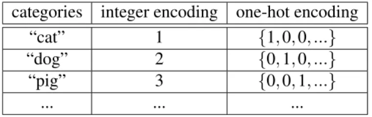
A classic example of a classification task is to correctly label pictures of different an-imals with the name of the animal. In classification problems, the targets express which of a set of categories (e.g. “dog”, “cat”, “pig”, ...) the inputs belong to. The number of categories, k, is typically finite and can thus be identified with the integers {1, 2, ..., k}. Another common way to represent categories in a classification problem is called the
6I’ve imprecisely conflated cost with reward in this discussion; while there is a significant difference between these concepts, a reward function can be translated into a cost function, given a perfect model of the world.
one-hot encoding. Here, we represent each category by a different k-dimensional binary vector with a 1 in one dimension and 0s in all the others (see table 2.II).
Table 2.II: Encoding categories as mathematical objects
categories integer encoding one-hot encoding
“cat” 1 {1, 0, 0, ...}
“dog” 2 {0, 1, 0, ...}
“pig” 3 {0, 0, 1, ...}
... ... ...
A common cost function for classification problems is called categorical cross-entropy. This is the cross entropy between the target and the prediction, considered as categorical (a.k.a “multinoulli”) distributions. Cross entropy is defined as:
H(p, q) = −
Z
p(x) log q(x)dx
which in the categorical case simply becomes − log q(t) where t is the target category; this is also called the negative log-likelihood7. The special case in which there are two categories is called binary classification.
2.2.6.2 Regresssion
In regression tasks, the targets are real-valued vectors (typically finite-dimensional). The example of predicting the value of the S&P500, from the beginning of this chapter, is a regression problem. The example of predicting the pixel values of the top half of an image given the bottom half is as well. A common cost function for regression is the mean squared error (MSE), given by the (average) squared distance between each prediction and its corresponding target:
MSE(X ,Y ) = E( f (x) − y)2
7A likelihood is simply a probability distribution at some point in its domain, considered as a function of the parameters of the distribution.
2.2.6.3 Structured output
Structured output refers to problems where the space of targets is structured (e.g. not categorical or scalar real-values). Predicting the pixel values of the top half of an image given the bottom half is a structured output problem, since the values of nearby pixels in images are correlated. Predicting multiple categorical variables is also a structured out-put problem (for instance, predicting which animal is in a picture, and which direction it is facing). Predicting a graph, e.g. a parse tree is another example.
2.2.7 Examples of UL: density estimation, clustering 2.2.7.1 Density estimation
Density Estimation involves learning a function that maps inputs to their probability mass or density. Such a function can be used, e.g. in structured prediction to “clean up” the outputs of a supervised learning model. For instance, in translation, if we have a small number of documents translated from French to English (labeled data), but a much larger number of documents in English (unlabeled data), we can learn a translation model using SL on the labeled data, and learn a language model to perform density estimation on the unlabeled data. The language model simply tells us how probable each English sentence is, so we can use this to select translations of a given French sentence that make more sense in English. Concretely, we might use the translation model to generate a list of candidate translations and then choose the one which is the most probable English sentence.
2.2.7.2 Clustering
A standard example of unsupervised learning is clustering. An exception to our definition of unsupervised learning above, Clustering methods don’t necessarily learn a probability distribution. Rather, they learn a function that assigns data points to corre-sponding clusters. Clusters can be thought of as an equivalence relation over data points; data points which are assigned to the same cluster are meant to be similar in some sense.
For instance, customers of some company might be clustered together based on their consumer habits and advertisements designed for each cluster.
One popular method for clustering is called k-means clustering. In k-means clus-tering, we decide in advance the number of clusters, k, and assign them each some point in data space. Then we assign data points to the nearest cluster, then move each cluster to the mean of the points assigned to it. We repeat this process until the assignments and means stop changing, which is guaranteed to happen after a finite number of iterations.
2.3 Optimization (minimizing cost)
We’ve defined learning as a search process over a space of functions. We call the process of searching for functions that minimize the cost function optimization, and a technique for performing optimization an optimizer8.
We view this search process as constructing sequence F = f1, f2, ... of candidate
functions, from which we take the element with minimum cost.
When the space F is finite, it is possible to search using brute-force; this is also called exhaustive search. When F is infinite, a simple strategy would be to place a probability distribution onF , and then sample functions from it; this is called random search.
Random search and exhaustive search are quite limited. Better search methods are the main thing that makes machine learning techniques seem intelligent. For exam-ple, the game of Go is the best-known classic game in which AI has not achieved super-human performance 9, and has received a large amount of attention among AI researchers. Because there is a maximum number of turns in a game of Go, and a finite number of possible moves per game, there are a finite number of possible games, and a finite number of strategies. Thus the best strategy could be found via exhaustive search. However, the number of strategies is also significantly larger than the number of
parti-8This is inspired by the idea of finding a local or global optimum (in this case a minimum) of the cost function, although in practice we are simply trying to improve upon the best function found so far, and don’t necessarily care if we have reached an optimum.
9Although recently, ? ] demonstrated significant progress, and super-human performance appears immanent.
cles in the known universe, so this exhaustive search could not be performed in practice using current technology.
A more interesting idea is local search, which we can think of as taking small steps through the space of functions, and adding the function at each step to the sequence F. This requiresF to have some structure; for instance if F is parametrized by k real numbers, then we can think of the space of functions as Rk; we will assume this is the case from here on. Local search methods include hill-climbing (adjusting a single parameter at each step in a way that decreases cost), and gradient descent.
Gradient descent uses the gradient of the cost with respect to the parameters: dLdθ , to find the direction of steepest descent. A learning rate, αt helps determine the step-size,
and can be constant, changed according to some predetermined schedule, or chosen by some more sophisticated method that aims to find the optimal step-size, such as a line search10. The formula for gradient descent, then, is:
θt+1= θt− αt
dL dθt
(2.1) Gradient descent methods are far and away the most popular way of optimizing ANNs. Initialization (how the first candidate function is chosen) is often important in local search, and has been shown to play a critical role in deep learning. Another natu-ral idea is to use multiple paths, initialized at different locations, to search the space of functions.
Local search is an example of an iterative method, in which each new function is expected to be an improvement over all previous functions considered. Consistently decreasing the cost at each time-step is an attractive property, but may not be enough to find a good solution. The best solutions are global minima, functions whose cost is minimal. A simple property that guarantees convergence to a global minimum is
10When training ANNs, it is common for the experimenter to tune the learning rate interactively. This is part of what has been called the “black art” of deep learning, since experienced researchers are often better at making these adjustments.
convexity. A function f : X → R is convex if
f(tx1+ (1 − t)x2) ≤ t f (x1) + (1 − t) f (x2), ∀x1, x2∈ X, ∀t ∈ [0, 1].
A great deal of optimization research focuses on the convex case, which has a well-developed theory. Non-convex optimization is not understood nearly as well, although the success of deep learning has generated some interest. Methods developed for convex optimization are often used in non-convex optimization, despite the lack of theoretic guarantees that they enjoy in the convex case.
We say an optimizer converges if the sequence of functions it produces is convergent. When convergence to a global optimum cannot be proven, it is often possible to prove convergence to a local optimum, but local optima may be very suboptimal. Recent work [10] in deep learning suggests this may not be the case for DNNs, however.
The geometry of function space and parameter space may not correspond exactly; the natural gradient can correct for this discrepancy, but can also be more costly to compute. Techniques for approximating the natural gradient have been used successfully in DL.
2.4 Generalization, overfitting and regularization
A machine learning algorithm finds a function that does a good job of explaining the data it has observed, as measured by the cost. This function reflects the mathematical patterns that it has found in its observations. But apparent patterns are often coincidental, a result of random chance that doesn’t properly reflect the data generating process.11.
We don’t want our model to focus on such patterns; in other words, we want it to generalize to new data generated by the same process as its previous observations, not just memorize the right answers for the training set. Informally, a function which performs well on inputs that it has encountered, but fails to generalize well is said to be overfitting. The not-quite-opposite problem of underfitting occurs when a function fails
11 Apophenia is the human tendency to perceive patterns in random data [74]. One notable example is the clustering illusion, in which randomly distributed points appear to form clumps or clusters. His-torically, Londoners developed theories about bombing patterns in WWII. The clustering illusion has also been offered (controversially) as an explanation for apparent regional clusters of cancer cases [12]
to capture important patterns in the data it has encountered.
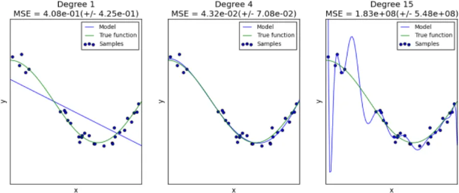
My favorite example for explaining overfitting and underfitting is polynomial regres-sion. In this setting, our model is an n-th degree polynomial. A higher degree polynomial can do a better job, even fitting the training data perfectly when n − 1 equals the number of data points, but this almost always is due to extreme overfitting; see figure 2.1.
Figure 2.1: Polynomial regression: The degree 1 polynomial (left) is too simple and underfits. The degree 15 polynomial (right) is too complicated and overfits. The degree 4 polynomial (middle) strikes a good balance between overfitting and underfitting. This figure is taken from [50].
2.4.1 Early stopping
One popular way of preventing overfitting with a finite dataset is early stopping. To perform early stopping, we randomly split our dataset into a three sets, called the training, validation, and test sets. We only train our model using the training set and perform model selection by evaluating cost on the validation set. Only once we have settled on a model and trained it (optionally using the validation set, as well) do we evaluate on the test set. The cost on the test set is then an unbiased evaluation of the trained model’s performance on unseen data from the data generating process.
2.4.2 Regularization
Early stopping is a form of regularization. A regularizer is a technique for prevent-ing overfittprevent-ing in a model by expressprevent-ing a preference among hypotheses. A common
form of regularizer adds a regularization term depending only on the hypothesis (and not the data) to the cost function.
The choice, made when selecting a model, of which hypotheses to consider, im-plicitly expresses a very strong prior, namely absolute certainty that the hypotheses not considered are incorrect. Just like the choice of model, regularization techniques express an inductive bias. Unlike model selection, regularization makes a ML algorithm favor certain hypotheses a priori, without completely removing any from consideration. Most regularizers introduce a new scalar hyperparameter specifying how strong the penalty should be, in effect expressing the confidence we have in the motivating inductive bias.
2.4.2.1 L1and L2regularization
Besides early stopping, another common way of regularizing is to encourage the pa-rameters to be small. For real-valued papa-rameters, larger values typically correspond to more extreme hypotheses, which are more likely to be overfit. The most common regu-larizers of this form penalize the L1 or L2 norm of the (real-valued) parameter vectors.
The L1 penalty has a tendency to encourage sparsity, meaning a large number of
pa-rameters are chosen to be 0. This means the trained model can often be compressed by removing these parameters.
When training a model with gradient descent, early stopping can be viewed as an adaptive form of L2 regularization, which chooses the strength of the penalty based on
the validation cost12.
These penalties have been used for neural nets, but are less common since the inven-tion of dropout regularizainven-tion [25].
2.4.3 Occam’s razor and model complexity
Perhaps the most general prior is a preference for simpler models. Occam’s Ra-zor states that between two theories which explain our observations, we should choose the simpler theory. More specifically, there is a trade-off between how well a pattern
explains the data, and how simple the model is 13. As suggested by the polynomial example, a simpler hypothesis often does a better job of generalizing. While regulariza-tion expresses a preference among hypotheses, we can also enforce a hard limit on the complexity of the hypotheses we consider. Removing more complex hypotheses from consideration should reduce overfitting, but what we ultimately care about in machine learning is generalization, not simplicity. Simplicity can also hurt generalization; if we do not consider the correct hypothesis because it is too complex, then our model is bound to underfit.
The concept of model complexity or model capacity corresponds to (inverse) sim-plicity in the sense of Occam’s Razor. A model with more parameters is often more complex, but more sophisticated methods of evaluating complexity may be necessary; models can be over-parametrized, meaning equivalent to a model with fewer parame-ters. A simple example is the function f (x) = θ1θ2x, with parameters θ1, θ2∈ R; any
such function could also be expressed with a single real-valued parameter θ = θ1θ2. In
fact, considering the same function, now with θ1∈ [0, 1], θ2 ∈ {−1, 1}, this model is
lessexpressive than the model given by f (x) = θ x, where θ can take on any real value, despite having more parameters.
There are more sophisticated theoretical notions of complexity, such as minimum description length (MDL), which measures how many bits it takes to encode a complete description of a model, and VC dimension, which measures how many points a binary classification model can shatter, i.e. classify correctly for any possible labeling, but there is no universally applicable method of comparing model complexity in practice.
When we have little prior knowledge about the data generating process, limiting the complexity of the model can be one of the best ways to prevent overfitting. For instance, a smaller neural network (i.e. one with fewer parameters) sometimes gives better performance, even with early stopping.
2.4.4 Risk minimization
We’ve defined learning as a search for functions with low cost. The principle of risk minimization states that the cost we should seek to minimize should depend on the data generating process, not the observed data. Since the data generating process is generally unknown, this cost cannot be evaluated directly. Structural risk minimization (SRM) provides a theoretical justification for using the cost on the training data (called the empirical risk) as a proxy for risk The trick is to control model complexity using the VC dimension. Specifically, the risk can be bounded (with some probability) by the empirical risk and the VC confidence. The VC confidence is a function of the VC dimension and the desired confidence that the bound holds (more confidence results in a looser bound).
Support Vector Machines (SVMs) are a popular algorithm based on the principles of SRM. Calculating the VC dimension for ANNs is not straightforward or common in current practice.Early stopping is similar in spirit to SRM, however; the complexity of an ANN generally increases through training, as it has more time to grow its parameter values14.
2.4.5 Bias and variance
Formally, we can view overfitting and underfitting as describing the bias and variance of the outputs of a learning procedure as a function of the training data. We view the learned function as a statistical estimator of a true function, and ask ourselves: if we were to receive a new dataset from the same generating process, how would our results change? High variance means that the function learned would be very different if it were trained on another dataset. High bias means that the result is suboptimal in some consistent way, regardless of what training data has been observed. This decomposition demonstrates how overfitting and underfitting are not opposites: a particularly bad model (e.g. with high complexity and a poor inductive bias) can suffer from both, whereas a good model will not suffer too much from either, given sufficient training data. When
14ANN parameters are usually initialized to values close to 0. Absent any regularization, the parameters generally grow throughout training.
there is not enough data to observe the trends one hopes to learn about, it is still possible to have a good model, with sufficient prior knowledge; in the limit of no data, this means knowing the correct function in advance.
2.5 The ML research process
The process of ML research tends to progress as follows: repeat
choose: task, training cost, evaluation cost, model, learning algorithm train the model using the learning algorithm and training cost
compute the evaluation cost of the learned function until satisfied or out of time/patience
Depending on the goal of the research project, frequently only one of the task, cost functions, model, or learning algorithm will be manipulated in the research loop, while the others are held fixed. It is important to remember that components can interact to determine which function is learned, however.
It is common to use good results from previous work as a baseline to compare against. Common research objectives are:
• evaluating the generality of a method (by comparing across tasks) • finding which of several methods performs better on a specific task
• gauging the robustness of one component to changes in the others (e.g. asking: how does my learning algorithm work with a different model?)
This approach has the advantage of allowing relatively straightforward comparison of different methods. However, each time we repeat the process, the learning algorithm starts over from scratch. This contrasts sharply with the life-long learning that animals exhibit, and that is desirable for many systems in practice. There is some work that attempt to transfer knowledge across tasks, but very few projects simulate an ongoing perpetual learning process. Also, as mentioned above, for real systems, it is necessary
to consider the appropriateness of the evaluation cost as a measure of task performance; the algorithm with the best evaluation cost might not be the one you want to use in your real-world system.
CHAPTER 3
DEEP LEARNING AND REPRESENTATION LEARNING
The phrase “deep learning” has been the subject of some controversy [59]. Bengio [5] defines depth via “the number of levels of composition of non-linear operations in the function learned”; According to this definition, which we call the technical definition, training any model with depth greater than one is deep learning. In practice, the phrase has been applied imprecisely to a wide range of work, starting with deep belief networks (DBNs) [24]. Most but not all of this work uses deep artificial neural networks (ANNs). In this chapter, we’ll describe feedforward ANNs (FNNs) and their relation to rep-resentation learning. We’ll also cover some of the most basic and important methods of deep learning.
3.1 Artificial neural networks
3.1.1 Biological inspirations and analogies
Artificial neural networks (ANNs) encompass a variety of machine learning models inspired by neuroscientific knowledge of how real biological neurons work1. In partic-ular, the activation of the “neurons” in an ANN can be thought of as representing the firing rate of a biological neuron2.
ANNs are, however, a gross simplification of biological neural networks. There are many different types of neurons and neurotransmitters in the brain, with different properties. But the most glaring difference in my mind is that ANNs operate in discrete
1ANNs are usually referred to simply as “neural nets” by deep learning researchers, but should be dis-tinguished from the biological neural networks that exist in the brain, as well as spiking neural networks, a more detailed model inspired by biological neural networks that operates in continuous time.
2Neurons are believed to communicate via binary electro-chemical signals called action potentials, or spikes; the firing rate is the number of spikes per unit of time. Some neuroscientists believe that all the information a neuron transmits is encoded in the firing rate, but assessing this claim is not straightfor-ward, and others believe the precise timing of the spikes also carries information. In particular, how to convert a spike-train (a signal of electric potential at the neuronal membrane) into a signal specifying the instantaneous firing rate is controversial [75].
time; I know of no justification for modeling a biological neural network this way, other than convenience.
3.1.2 Neural net basics
An ANN is a weighted (directed or undirected) graph, whose nodes represent neu-rons (and are often called units), and whose edges represent synapses and are called weights or connections. The ANN architectures we consider in this thesis are directed graphs with inputs as roots and outputs as leaves. Each neuron is computed as a (possibly random, but usually deterministic) function of its parents.
Each neuron computes its activation as a function of its parents’ activations. The activations are transient and input-dependent; they are not parameters. The parameters of the network determine which functions the neurons compute. The activation of a neuron is typically computed as a linear function (i.e. a weighted sum) of its inputs (called the preactivation) followed by a nonlinearity; see figure 3.1 for a depiction of this computation.
Figure 3.1: The computation performed by a single neuron in a neural network. This figure is adapted from [73].
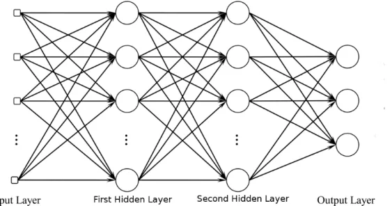
In the most basic standard ANN architecture, called the multi-layer perceptron (MLP), neurons are organized into fully connected layers, which share parents and chil-dren (see figure 3.2). Since each unit typically has a (nonlinear) activation function, σ ,
(also called a nonlinearity), each layer of units increases the depth of the architecture.
Figure 3.2: The computational graph of an MLP with two hidden layers and three output units. This figure is adapted from [58].
The weights on an ANN specify the strength of the connections between neurons. We typically add a constant bias term to the preactivation of each neuron; this is equivalent to giving all neurons a parent with a fixed activation of 1. The weights for each layer are organized into a weight matrix, with rows corresponding to parents and columns, chil-dren. Each entry in this matrix then corresponds to one edge of the computational graph. This allows the computations each layer of neurons performs to be written compactly as:
h= σ (W x + b)
where h are the activations of the child layer, x the parents’ activations, and the param-eters are W and b: the weight matrix and vector of bias terms, respectively (σ is the layer’s activation function). When we have have more than two layers, we denote the in-put layer as x, the outin-put layer, y, and the i-th hidden layer as hi. We index nonlinearities
and parameters similarly, so we can write the computation a FNN with l hidden layers performs in closed form as follows:
y= σy(Wyhl+ by) (3.1)
y= σy(Wyσl(Wlhl−1+ bl) + by) (3.2)
y= σy(Wyσl(Wlσl−1(Wl−1(...σ1(W1x+ b1)... + bl−1) + bl) + by) (3.3)
For layers that are not fully connected (i.e. missing some edges between the parent and child layers), we can simply set the corresponding entries of the weight matrices to 0. Computational graphs are sometimes depicted with nodes representing layers as opposed to individual units.
3.1.3 Activation functions
Nonlinear activation functions are what make deep nets deep architectures. The com-position of linear (or affine) functions is itself a linear (or affine) function, so without nonlinearities, stacking multiple layers is redundant. The output nonlinearity must be compatible with the cost function, and the choice of hidden layer activation functions can have a dramatic effect on performance. Some activation functions, such as the soft-max, cannot be computed elementwise.
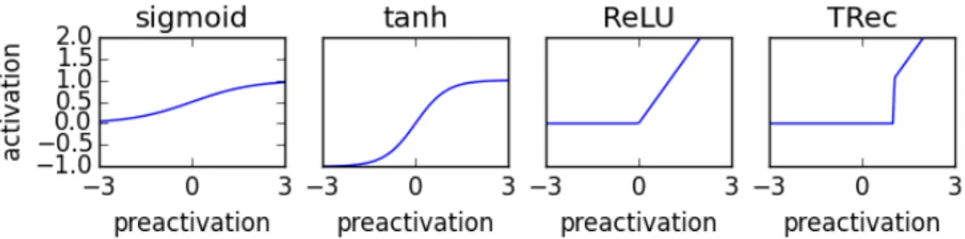
Figure 3.3: Common activation functions for neural nets, and the TRec activation func-tion with threshold 1.
3.1.3.1 Logistic sigmoid
The classical activation function is the logistic sigmoid (usually just called sigmoid), given by:
sigmoid(x) = 1 1 + e−x
The range of the sigmoid is (0, 1), and it is the default choice of output nonlinearity in bi-nary classification, where we typically interpret the output as representing the parameter of a Bernoulli distribution.
3.1.3.2 Hyperbolic tangent
The hyperbolic tangent (tanh) function is another s-shaped curve, but its range is (−1, 1). This activation function was traditionally used for recurrent connections, where it was found to outperform sigmoid. The equation for tanh is:
tanh(x) =1 − e
−2x
1 + e−2x 3.1.3.3 Softmax
The softmax activation function is used almost exclusively in the output layer. It converts a set of real numbers into the parameters of a categorical distribution, in such a way that increasing the preactivation of a unit always increases its activation (i.e. it is monotonic in every component). This is accomplished by first converting all the preac-tivations into positive real numbers with the exponential function, and then normalizing the result to sum to 1:
softmax(xj) =
exj ∑Kk=1exk
3.1.3.4 Rectified linear and variants
Widespread use of the rectified linear (ReLU) activation function is one of the more recent trends in training neural nets. This function is computed as
ReLU(x) = max(0, x)
ReLU generally significantly outperforms so called saturating nonlinearities, such as sigmoid and tanh 3. This may be because the gradients for saturating nonlinearities become very small when they are saturating (i.e. near their asymptotes). Since weights tend to increase during training, preactivations would typically increase as well, pushing these units into their saturating regime. For ReLU, negative preactivations give a gradient of 0, but in practice this doesn’t seem to be as much of an issue; since activations are input-dependent, most units should be active (i.e. non-zero) for some inputs, in which cases they have a significant gradient.
Due to its empirical success, several variants of ReLU have been explored [14, 23, 35, 40]. In this thesis, we use the TRec activation function [35], which is used without bias parameters, and instead has a “threshold” hyperparameter (set to 1 in the original paper and 0 in this thesis). The activation is then just given by:
TRec(x) = x(x > thresh).
3.2 Features and representations
The way data is presented to a learning algorithm, called a representation, has a large effect on results. Informally, we think of different mathematical objects as representing the same data. Formally, any (potentially random) function of a dataset can be thought of as transforming the dataset into a new representation. A feature map or feature detec-tor is a function that computes a new representation for each data point independently. The dimensions of such a representation are called features (although this term is also
3Having bounded activations is desirable in many settings, however, and so saturating nonlinearities remain widely used.
commonly used to refer to feature maps). Not all representations can be decomposed in this way, however; for instance, a dataset of M N-dimensional real vectors might be transformed by subtracting the global mean of all MN scalar values from each vector. The process of using feature maps to create a new representation of a data point is called feature extraction.
There is no single metric for the quality of a given representation, and in practice, quality is task-dependent. Nonetheless, there are several ways in which representations can be evaluated, and proven to be more or less useful.
• human-interpretability: Facilitating human understanding or visualization is use-ful. Descriptive statistics is mostly used for this purpose. Projecting high-dimensional data into 2-dimensional space for visualization using t-SNE [68] is one example. • independence of features: Statistically independent features can be thought of as
disentangling underlying factors of variation, i.e. the higher-level concepts that are important for understanding the world. The idea of natural kinds in philoso-phy expresses a similar idea. A classic example is expression and pose for pictures of human faces.
• compression: Compression of data reduces storage and communication costs. • sparsity: A sparse representation, with fewer active components, could greatly
reduce computation, and facilitate compression.
• performance in pipeline: Often, the ultimate measure of the utility of a represen-tation is simply the performance in some task of interest we get using that repre-sentation. We call the entire system including the transformation of raw data into a new representation and the algorithm that learns to perform the task a pipeline. Machine learning practitioners often use domain knowledge to specify the choice of representation directly, a process called feature engineering. Using machine learning to search for good representations is called representation learning4. Bengio et al. [6]
4Unfortunately, the acronym RL in ML is already claimed by reinforcement learning. Still, sometimes RL is used to refer to representation learning, but I avoid it.
argue that generic inductive biases for representation learning are important for develop-ing more general AI, and give several examples of such inductive biases, some of which can be used to motivate deep learning techniques. Powerful and generic representation learning techniques would allow an algorithm to learn task-relevant representations with minimal human guidance.
While most common representation learning techniques learn feature maps, the fea-ture learning process typically depends very much on the entire dataset, since we want the features to do a good job of representing any data that is likely to be sampled from the data distribution.
3.2.1 Deep learning and representation learning
In ANNs, every unit/neuron represents a feature map. Most of the power of DNNs comes from the representations they learn. DNNs learn a feature hierarchy, where higher order features (those computed after the first hidden layer) are computed as a function of features from the layer below. In most recent work, all features are learned jointly using supervised learning and SGD. The top layers of DNNs generally use the same basic linear classification or regression functions as previous methods; DNNs out-perform other methods because they have better features.
A DNN learns a representation that is both deep and distributed [6]. These character-istics of their architecture encode a prior almost as generic as locality, but considerably more powerful.
Traditional clustering techniques (see 2.2.7.2) have a many-to-one mapping from inputs to features, and are not distributed. Distributed representations represent different inputs with a combination or code of features, as opposed to just one. This is related to the independence prior we mentioned above; different aspects of an input can often be varied (almost) independently. For instance we could represent a car in terms of its color, condition, etc. As a human, when we see a model of car we’ve never seen before, it might be somewhat surprising, but seeing that same model in a different color or condition afterwards is not. As this example is meant to demonstrate, distributed representations allow for non-local generalization.
![Figure 3.1: The computation performed by a single neuron in a neural network. This figure is adapted from [73].](https://thumb-eu.123doks.com/thumbv2/123doknet/7645508.236993/37.918.185.739.629.896/figure-computation-performed-single-neuron-neural-network-adapted.webp)