OATAO is an open access repository that collects the work of Toulouse
researchers and makes it freely available over the web where possible
Any correspondence concerning this service should be sent
to the repository administrator:
[email protected]
This is an author’s version published in:
https://oatao.univ-toulouse.fr/26276
To cite this version:
Balbiani, Philippe and Boudou, Joseph and Diéguez, Martín and
Fernández Duque, David Intuitionistic linear temporal logics.
(2019) ACM Transactions on Computational Logic, 21 (2). ISSN
1529-3785
Open Archive Toulouse Archive Ouverte
Official URL :
https://doi.org/10.1145/3365833
Intuitionistic Linear Temporal Logics
Philippe Balbiani.
∗1, Joseph Boudou.
†1, Mart´ın Di´eguez
‡2, and
David Fern´
andez-Duque
§31
IRIT, Toulouse University. Toulouse, France
2
CERV, ENIB,LAB-STICC. Brest, France
3
Department of Mathematics, Ghent University. Gent, Belgium
Abstract
We consider intuitionistic variants of linear temporal logic with ‘next’, ‘until’ and ‘release’ based on expanding posets: partial orders equipped with an order-preserving transition function. This class of structures gives rise to a logic which we denote ITLe, and by imposing additional constraints we obtain the logics ITLp
of persistent posets and ITLht of here-and-there temporal logic,both of which have been considered in the literature. We prove that ITLehas the effective finite model property and hence is decidable, while ITLp does not have the finite model property. We also introduce notions of bounded bisimulations for these logics and use them to show that the ‘until’ and ‘release’ operators are not definable in terms of each other, even over the class of persistent posets.
1
Introduction
Intuitionistic logic [9, 35] and its modal extensions [16, 41, 44] play a crucial role in computer science and artificial intelligence and Intuitionistic Temporal Log-ics have not been an exception. The study of these logLog-ics can be a challenging enterprise [44] and, in particular, there is a huge gap that must be filled regard-ing combinations of intuitionistic and linear-time temporal logic [42]. This is especially pressing given several potential applications of intuitionistic temporal logics that have been proposed by several authors.
The first involves the Curry-Howard correspondence [24], which identifies intuitionistic proofs with the λ-terms of functional programming. Several ex-tensions of the λ-calculus with operators from Linear Time Temporal Logic [42]
∗ [email protected] † [email protected] ‡ [email protected] § [email protected]
(LTL) have been proposed in order to introduce new features to functional lan-guages: Davies [10, 11] has suggested adding a ‘next’ (◯) operator to intu-itionistic logic in order to define the type system λ◯, which allows extending functional languages with staged computation1
[15]. Davies and Pfenning [12] proposed the functional language Mini-ML◻ which is supported by intuitionistic S4and allows capturing complex forms of staged computation as well as runtime code generation. Yuse and Igarashi later extended λ◯to λ◻ [45] by incorporat-ing the ‘henceforth’ operator (◻), useful for modelling persistent code that can be executed at any subsequent state.
Alternately, intuitionistic temporal logics have been proposed as a tool for modelling semantically-given processes. Maier [33] observed that an intuition-istic temporal logic with ‘henceforth’ and ‘eventually’ (◇) could be used for reasoning about safety and liveness conditions in possibly-terminating reactive systems, and Fern´andez-Duque [18] has suggested that a logic with ‘eventu-ally’ can be used to provide a decidable framework in which to reason about topological dynamics. In the areas of nonmonotonic reasoning, knowledge repre-sentation (KR), and artificial intelligence, intuitionistic and intermediate logics have played an important role within the successful answer set programming (ASP) [7] paradigm for practical KR, leading to several extensions of modal ASP [8] that are supported by intuitionistic-based modal logics like temporal here and there [3].
There have been some notable steps towards understanding intuitionisitic temporal logics:
• Davies’ intuitionistic temporal logic with ◯ [10] was provided Kripke se-mantics and a complete deductive system by Kojima and Igarashi [27]. • Logics with◯, ◻ were axiomatized by Kamide and Wansing [25], where ◻
was interpreted over bounded time.
• Balbiani and Di´eguez [3] axiomatized the Here and There [22] variant of LTLwith◯, ◇, ◻.
• Davoren [13] introduced topological semantics for temporal logics and Fern´andez-Duque [18] proved the decidability of a logic with ◯, ◇ and a universal modality based on topological semantics.
Nevertheless, many questions have remained open, especially regarding conser-vative extensions of intuitionistic logic with all of the tenses◯, ◇, ◻, or even the more expressive ‘until’ U and ‘release’ R.
With the exception of [13, 18], semantics for intuitionistic LTL use frames of the form(W, ≼, S), where ≼ is a partial order used to interpret the intuitionistic implication and S is a binary relation used to interpret temporal operators. Since we are interested in linear time, we will restrict our attention to the case where S is a function. Thus, for example, ◯p is true at some world w ∈ W whenever p is true at S(w). Note, however, that S cannot be an arbitrary
1
Staged computationis a technique that allows dividing the computation in order to exploit the early availability of some arguments.
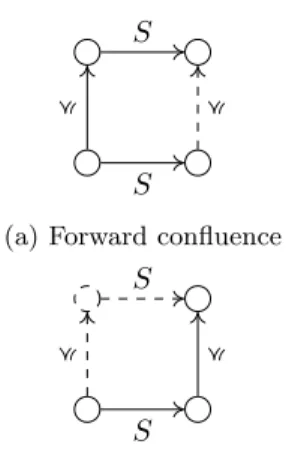
function. Intuitionistic semantics have the feature that, for any formula ϕ and worlds w ≼ v ∈ W , if ϕ is true at w then it must also be true at v; that is, truth is monotone (with respect to≼). If we want this property to be preserved by formulas involving ◯, we need for ≼ and S to satisfy certain confluence properties. In the literature, one generally considers frames satisfying
1. w≼ v implies S(w) ≼ S(v) (forward confluence, or simply confluence), and 2. if u≽ S(w), there is v ≽ w such that S(v) = u (backward confluence) (see Figure 1). We will call frames satisfying these conditions persistent frames (see Sec. 3), mainly due to the fact that they are closely related to (persistent) products of modal logics [30]. Persistent frames for intuitionistic LTL are closely related to the frames of the modal logic LTL×S4, which is non-axiomatizable. For this reason, it may not be surprising that it is unknown whether the intuitionistic temporal logic of persistent frames, which we denote ITLp, is decidable.
However, as we will see in Proposition 1, only forward confluence is needed for truth of all formulas to be monotone, even in the presence of◇, ◻ or even U and R. The frames satisfying this condition are, instead, related to expand-ing products of modal logics [20], which are often decidable even when the corresponding product is non-axiomatizable. This suggests that dropping the backwards confluence could also lead to a more manageable intuitionistic tem-poral logic. We denote the resulting logic by ITLe and, as we will prove in this
paper, it enjoys a crucial advantage over ITLp: ITLehas the effective finite model
property (hence it is decidable), but ITLp does not. In fact, to the best of our
knowledge, ITLeis the first known decidable intuitionistic temporal logic that
1. is conservative over propositional intuitionistic logic, 2. includes (or can define) the three tenses◯, U, R, and 3. is interpreted over infinite time.
Intuitively, ITLpis a logic of invertible processes, while ITLe reasons about
non-invertible ones. The latter is closely related to ITLc, an intuitionistic temporal
logic for continuous dynamic topological systems [18]. In contrast, the logic ITLe is based on relational, rather than topological, semantics, which has the
advantage of admitting a natural ‘henceforth’ operator (although topological variants can be defined [6]). The current work extends previous results regarding a variant of ITLe with◇ and ◻, rather than U and R [5].
Note that◇ϕ ≡ ¬◻¬ϕ is not valid intuitionistically and hence ◇ cannot be defined in terms of◻ using the standard equivalence. The same situation holds for the ‘until’ operator: while the language with◯ and U is equally expressive to classical monadic first-order logic with≤ over N [19], U admits a first-order definable intuitionistic dual, R (‘release’), which cannot be defined in terms of Uusing the classical definition.
However, this is not enough to conclude that R cannot be defined in a differ-ent way in terms of U. Thus we will consider the question of definability: which
of the modal operators can be defined in terms of the others? As is well-known, ◇ϕ ≡ ⊺ U ϕ and ◻ϕ ≡ R ϕ; these equivalences remain valid in the intuitionistic setting. Nevertheless, we will show that◻ cannot be defined in terms of U, and ◇ cannot be defined in terms of R; in order to prove this, we will develop a theory of bisimulations on ITLe models.
Layout
The paper is organised as follows: in Section 2 we present the syntax and the semantics in terms of dynamic posets and also study the validity of some of the classical axioms in our setting. In Section 3 we present the concepts of stratified and expanding frames and also show that satisfiability and validity on arbitrary models is equivalent to satisfiability and validity on expanding models. In Section 4 we consider two smaller classes of models, persistent and here-and-there models, and we compare their logics to ITLe.
The Finite Model Property of ITLeis studied along sections 5 and 6. In the
former we introduce the concepts of labelled structures and quasimodels as well as several related concepts such as immersions, condensations, and normalised quasimodels. Those definitions are used in Section 6 to prove the finite model property of ITLe.
In Section 7 we define the concept of bounded bisimulations in intuitionistic modal setting and use them to study the interdefinability of the ITLemodalities
in Section 8. We finish the paper with conclusions and future work.
2
Syntax and semantics
We will work in sublanguages of the language L given by the following grammar: ϕ, ψ∶= p ∣ ∣ (ϕ∧ψ) ∣ (ϕ∨ψ) ∣ (ϕ → ψ) ∣ (◯ϕ) ∣ (◇ϕ) ∣ (◻ϕ) ∣ (ϕ U ψ) ∣ (ϕ R ψ) where p is an element of a countable set of propositional variables P. Henceforth we adhere to the standard conventions for omission of parentheses. All sublan-guages we will consider include all Boolean operators and◯, hence we denote them by displaying the additional connectives as a subscript: for example, L◇◻
denotes the U-free, R-free fragment. As an exception to this general convention, L◯ denotes the fragment without◇, ◻, U or R.
Given any formula ϕ, we define the length of ϕ (in symbols,∣ϕ∣) recursively as follows:
• ∣p∣ = ∣∣ = 0;
• ∣φ ⊙ ψ∣ = 1 + ∣φ∣ + ∣ψ∣, with ⊙ ∈ {∨, ∧, →, R, U}; • ∣⊙ψ∣ = 1 + ∣ψ∣, with ⊙ ∈ {¬, ◯, ◻, ◇}.
Broadly speaking, the length of a formula ϕ corresponds to the number of connectives appearing in ϕ.
S S
≼ ≼
(a) Forward confluence
S
≼
S
≼
(b) Backward confluence
Figure 1: On a dynamic poset the above diagrams can always be completed if S is forward or backward confluent, respectively. Posets with both properties are persistent.
2.1
Dynamic posets
Formulas of L are interpreted over dynamic posets. A dynamic poset is a tuple D= (W, ≼, S), where W is a non-empty set of states, ≼ is a partial order, and S is a function from W to W satisfying the forward confluence condition that for all w, v∈ W, if w ≼ v then S(w) ≼ S(v). An intuitionistic dynamic model, or simply model, is a tuple M= (W, ≼, S, V ) consisting of a dynamic poset equipped with a valuation function V ∶ W Ð→ ℘ (P) that is monotone in the sense that for all w, v∈ W, if w ≼ v then V (w) ⊆ V (v). In the standard way, we define S0
(w) = w and, for all k≥ 0, Sk+1(w) = S (Sk(w)). Then we define the satisfaction relation
⊧inductively by: 1. M, w ⊧ p iff p∈ V (w); 2. M, w⊭ ; 3. M, w ⊧ ϕ∧ ψ iff M, w ⊧ ϕ and M, w ⊧ ψ; 4. M, w ⊧ ϕ∨ ψ iff M, w ⊧ ϕ or M, w ⊧ ψ; 5. M, w ⊧◯ϕ iff M, S(w) ⊧ ϕ; 6. M, w ⊧ ϕ → ψ iff∀v ≽ w, if M, v ⊧ ϕ, then M, v ⊧ ψ; 7. M, w ⊧◇ϕ iff there exists k ≥ 0 such that M, Sk(w) ⊧ ϕ;
8. M, w ⊧◻ϕ iff for all k ≥ 0 we have that M, Sk(w) ⊧ ϕ;
9. M, w ⊧ ϕ U ψ iff there exists k≥ 0 such that M, Sk(w) ⊧ ψ and ∀i ∈[0,k),
M, Si(w) ⊧ ϕ;
10. M, w ⊧ ϕ R ψ iff for all k≥ 0, either M, Sk(w) ⊧ ψ or ∃i ∈ [0,k) such that
w
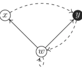
x y
Figure 2: Example of an ITLe model M=(W,≼,S,V ), where ≼ is the reflexive
and transitive closure of the relation indicated by the solid arrows, S is the relation indicated by the dashed arrows, and a black dot indicates that the variable p is true, so that we only have p∈ V(y). Then, the reader may verify that M, x ⊧◯p but M, x ⊭ p, while M, y ⊧ p but M, y ⊭ ◯p. From this it follows that M, w⊭(◯p → p) ∨ (p → ◯p).
See Figure 2 for illustration of the ‘⊧’ relation. Given a model M=(W,≼,S,V ) and w∈ W , we write ΣM(w) for the set {ψ ∈ Σ ∣ M,w ⊧ ψ}; the subscript ‘M’
is omitted when it is clear from the context.
A formula ϕ is satisfiable over a class Ω of models if there is a model M∈ Ω and a world w so that M, w ⊧ ϕ, and valid over Ω if, for every world w of every model M∈ Ω we have that M, w ⊧ ϕ. Satisfiability (resp. validity) over the class of all intuitionisitic dynamic models is called satisfiability (resp. validity) for the expanding domain intuitionisitic temporal logic ITLe. We will justify this
terminology in the next section. First, we remark that dynamic posets impose the minimal conditions on S and≼ in order to preserve the monotonicity of truth of formulas, in the sense that if M, w ⊧ ϕ and w≼ v then M, v ⊧ ϕ. Below, we will use the notation JϕK={w ∈ W ∣ M,w ⊧ ϕ}.
Proposition 1. Let D=(W,≼,S), where (W,≼) is a poset and S∶W → W is any function. Then, the following are equivalent:
1. S is forward confluent;
2. for every valuation V on D and every formula ϕ, truth of ϕ is monotone with respect to≼.
Proof. That (1) implies (2) follows by a standard structural induction on ϕ. The case where ϕ ∈ P follows from the condition on V and most inductive steps are routine. Consider the case where ϕ= ψ U θ, and suppose that w ≼ v and w ∈ JϕK. Then there exists k ∈ N such that M, Sk(w) ⊧ θ and for all
i∈[0,k), M,Si(w) ⊧ ψ. Since S is confluent, an easy induction shows that, for
all i∈[0,k], Si(w) ≼ Si(v). Therefore, from the induction hypothesis we obtain
that M, Sk(v) ⊧ θ and for all i ∈ [0,k), M,Si(v) ⊧ ψ. Other cases are either
similar or easier.
Now we prove that (2) implies (1) by contrapositive. Suppose that(W,≼,S) is not forward-confluent, so that there are w≼ v such that S(w) /≼ S(v). Choose p∈ P and define V(u) = {p} if S(w) ≼ u, V (u) = ∅ otherwise. It follows from
w v
u
Figure 3: A dynamic intuitionistic model. As in the previous figure, solid arrows represent the intuitionistic order≼, dashed arrows the successor relation S, the black point satisfies the atom p and no point satisfies any other atom. Note that Sis forward, but not backward, confluent. The world w satisfies¬ ◯ p ∧ ¬ ◯ ¬p.
the transitivity of≼ that V is monotone. However, p/∈ V (S(v)), from which it follows that(D,V ),w ⊧ ◯p but (D,V ),v ⊭ ◯p.
Observe that satisfiability in propositional intuitionistic logic is equivalent to satisfiability in classical propositional logic. This is because, if ϕ is classi-cally satisfiable, it is trivially intuitionisticlassi-cally satisfiable in a one-world model; conversely, if ϕ is intuitionistically satisfiable, it is satisfiable in a finite model, hence in a maximal world of that finite model, and the generated submodel of a maximal world is a classical model. Thus it may be surprising that the same is not the case for intuitionistic temporal logic:
Proposition 2. Any formula ϕ of the temporal language that is classically sat-isfiable is satsat-isfiable in a dynamic poset. However, there is a formula satsat-isfiable on a dynamic poset that is not classically satisfiable.
Proof. If ϕ is satisfied on a classical LTL model M, then we may regard M as an intuitionistic model by letting≼ be the identity. On the other hand, consider the formula¬ ◯ p ∧ ¬ ◯ ¬p (recall that ¬θ is a shorthand for θ → ). Classically, this formula is equivalent to¬ ◯ p ∧ ◯p, and hence unsatisfiable. Define a model M=(W,≼,S,V ), where W = {w,v,u}, x ≼ y if x = y or x = v, y = u, S(w) = v and S(x) = x otherwise, V (u) = {p} and V (v) = V (w) = ∅ (see Figure 3). Then, one can check that M, w ⊧¬ ◯ p ∧ ¬ ◯ ¬p.
Hence the decidability of the intuitionistic satisfiability problem is not a corollary of the classical case. In Section 6, we will prove that both the satisfi-ability and the validity problems are decidable. We will prove this by showing that ITLe has the effective finite model property: recall that a logic Λ has the
effective finite model property for a class of models Ω if there is a computable function f∶ N → N such that given a formula ϕ, we have that ϕ is satisfiable (falsifiable) on Ω if and only if there is M∈ Ω such that ϕ is satisfied (falsified) on M and whose domain has at most f(∣ϕ∣) elements.
2.2
Some valid and non-valid ITL
eformulas
In this section we present some examples of valid formulas that will be useful throughout the text. We begin by focusing on formulas of L◇◻.
Proposition 3. The following formulas are ITLe-valid:
1. ◯ ↔ 2. ◯(ϕ ∧ ψ) ↔ (◯ϕ ∧ ◯ψ) 3. ◯(ϕ ∨ ψ) ↔ (◯ϕ ∨ ◯ψ) 4. ◯(ϕ → ψ) → (◯ϕ → ◯ψ) 5. ◯◻ϕ ↔ ◻ ◯ ϕ 6. ◯◇ϕ ↔ ◇ ◯ ϕ
Proof. We prove that 4 holds and leave other items to the reader. Let M= (W,≼,S,V ) be any dynamic model and w ∈ W be such that M,w ⊧ ◯(ϕ → ψ). Let v ≽ w be such that M, v ⊧ ◯ϕ. Then, M, S(v) ⊧ ϕ. But S(w) ≼ S(v) and M, S(w) ⊧ ϕ → ψ, so that M,S(v) ⊧ ψ and M,v ⊧ ◯ψ. Since v ≽ w was arbitrary, M, w ⊧◯ϕ → ◯ψ.
Note that, unlike the other items, 4 is not a biconditional, and indeed the converse is not valid over the class of all dynamic posets (see Proposition 6). Next we show that◇ϕ (resp. ◻ϕ) can be defined in terms of U (resp. R) and the LTL axioms involving U and R are also valid in our setting:
Proposition 4. The following formulas are ITLe-valid:
1. (ϕU ψ) ↔ ψ ∨ (ϕ ∧ ◯(ϕU ψ)) 2. (ϕR ψ) ↔ ψ ∧ (ϕ ∨ ◯(ϕR ψ)) 3. (ϕU ψ) → ◇ψ 4. ◻ψ →(ϕR ψ) 5. ◇ϕ ↔(⊺U ϕ) 6. ◻ϕ ↔(R ϕ) 7. ◯(ϕU ψ) ↔ (◯ϕ)U(◯ψ) 8. ◯(ϕR ψ) ↔ (◯ϕ)R(◯ψ) 9. ϕ U ψ ↔(ψ R(ϕ ∨ ψ)) ∧ ◇ψ 10. ϕ R ψ ↔(ψ U(ϕ ∧ ψ)) ∨ ◻ψ Proof. We consider some cases below. For (1), from left to right, let us assume that M, w ⊧ ϕ U ψ. Therefore there exists k≥ 0 s.t. M, Sk(w) ⊧ ψ and for all
j satisfying 0≤ j < k, M, Sj(w) ⊧ ϕ. If k = 0 then M,w ⊧ ψ while, if k > 0 it
follows that M, w ⊧ ϕ and M, S(w) ⊧ ϕU ψ. Therefore M,w ⊧ ψ∨(ϕ ∧ ◯ϕU ψ). From right to left, if M, w ⊧ ψ then M, w ⊧ ϕ U ψ by definition (with k= 0). If M, w ⊧ ϕ∧◯ϕ U ψ then M, w ⊧ ϕ and M, S(w) ⊧ ϕU ψ so, due to the semantics, we conclude that M, w ⊧ ϕ U ψ (with some k≥ 1). In any case, M, w ⊧ ϕ U ψ.
For (2), we work by contrapositive. From right to left, let us assume that M, w /⊧ ϕR ψ. Therefore there exists k ≥ 0 s.t. M,Sk(w) /⊧ ψ and for all j satisfying 0≤ j < k, M, Sj(w) /⊧ ϕ. If k = 0 then M,w /⊧ ψ while, if k > 0 it follows
that M, w/⊧ ϕ and M,S(w) /⊧ ϕR ψ. In any case, M,w /⊧ ψ∧(ϕ ∨ ◯ϕR ψ). From left to right, if M, w /⊧ ψ then M,w /⊧ ϕR ψ by definition. If M,w /⊧ ϕ ∨ ◯ϕR ψ then M, w /⊧ ϕ and M,S(w) /⊧ ϕU ψ so, due to the semantics of R, we conclude that M, w/⊧ ϕR ψ. In any case, M,w /⊧ ϕR ψ.
With these equivalences in mind, we can simplify the syntax of the full language L.
Proposition 5. The languages L◇R and L◻U are expressively equivalent to L
over the class of dynamic posets.
Proof. From the validities◻ϕ ↔ R ϕ and ϕ U ψ ↔(ψ R(ϕ ∨ ψ)) ∧ ◇ψ we see that any ϕ∈ L is equivalent to some ϕ′∈ L
◇R. Similarly, from◇ϕ ↔ ⊺ U ϕ and
ϕ R ψ ↔(ψ U(ϕ ∧ ψ)) ∨ ◻ψ we see that L◻U is expressively equivalent to L.
Nevertheless, we will later show that both LUand LRare strictly less
expres-sive than the full language, in contrast to the classical case.
3
The expanding model property
As mentioned in the introduction, the logic ITLeis closely related to expanding
products of modal logics [20]. In this subsection, we introduce stratified and expanding frames, and show that satisfiability and validity on arbitrary models is equivalent to satisfiability and validity on expanding models. To do this, it is convenient to represent posets using acyclic graphs.
Definition 1. A directed acyclic graph is a tuple (W,↑), where W is a set of vertices and ↑⊆ W × W is a set of edges whose reflexive, transitive closure ↑∗ is antisymmetric. We will tacitly identify (W,↑) with the poset (W,↑∗). A path from w1 to w2 is a finite sequence v0. . . vn∈ W such that v0= w1, vn = w2 and
for all k< n, vk↑vk+1. A tree is an acyclic graph(W,↑) with an element r ∈ W,
called the root, such that for all w∈ W there is a unique path from r to w. A poset(W,≼) is also a tree if there is a relation ↑ on W × W such that (W,↑) is a tree and≼ = ↑∗.
Below, if R ⊆ A × A is a binary relation and X ⊆ A, R⇂X denotes the
restriction of R to X. Similarly if f∶ A Ð→ B then f⇂X denotes the restriction
of f to the domain X.
Definition 2. A model M = (W,≼,S,V ) is stratified if there is a partition {Wn}n<ω of W such that
1. each Wn is closed under≼,
2. for all n,(Wn,≼⇂Wn) is a tree, and
3. if w∈ Wn then S(w) ∈ Wn+1.
If M is stratified, we write ≼n, Sn, and Vn instead of ≼⇂Wn, S⇂Wn, and V ⇂Wn.
We then define Mn = (Wn,≼n, Vn). If moreover we have that S(w) ≼ S(v)
implies w≼ v, then we say that M is an expanding model. We define stratified and expanding posets similarly, ignoring the clauses for V .
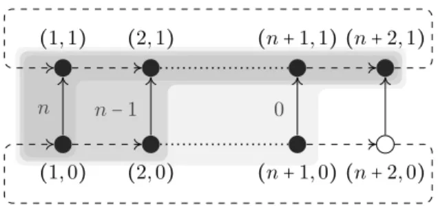
(0,0)w (1,0)x (2,0)y (0,1)w (1,1)y (2,1)w (3,1)x (4,1)y ⋯ ⋯ ⋯ ⋯ ⋯
Figure 4: The strata We 0, W
e
1 of the stratified model obtained from the model
defined in Figure 2. The subindices indicate the value of h=⋃k∈Nhk.
Below if Σ⊆ ∆ ⊆ L we write Σ ⋐ ∆ to indicate that Σ is finite and closed under subformulas. In view of Proposition 5, in this section we may restrict our attention to L◻U. Given Σ⋐ L◻U, a model M=(W,≼,S,V ), and a state w ∈ W,
we will construct a stratified model Me
=(We
,≼e
, Se
, Ve) such that for the root
we
of We 0, Σ(w
e) = Σ(w).
Definition 3. Let Σ⋐ L◻U and M=(W,≼,S,V ) be a model. We first define the
set D= N×N×℘(Σ) of possible defects, and fix an enumeration ((xk, yk, Hk))k∈N
of D; since Σ is finite and not empty, we assume that D is enumerated such that for each k > 0, xk ≤ k. Then, for each k ∈ N, we construct inductively a
tuple(Uk, ↑k, hk) where Uk⊆ N ×N, ↑k⊆ Uk× Uk and hk ∶ UkÐ→W. The model
Me is defined from these tuples and the whole construction proceeds as follows:
Base case. Let U0={0} × N, ↑0= ∅ and h0 be such that for all (0,y) ∈ U0,
h0(0,y) = Sy(w).
Inductive case. Let k ≥ 0 and suppose that (Uk, ↑k, hk) has already been
constructed. Let(x,y,H) = (xk, yk, Hk). If (D1) (x,y) ∈ Uk and (D2) there is
v= vk∈ W such that hk(x,y) ≼ v and Σ(v) = H, then we construct (Uk+1, ↑k+1
, hk+1) such that:
Uk+1= Uk∪{(k + 1,a) ∣ y ≤ a ∈ N}
↑k+1= ↑k∪{((x,a),(k + 1,a)) ∣ y ≤ a ∈ N} hk+1= hk∪{((k + 1,a),Sd−y(v)) ∣ y ≤ d ∈ N}
Otherwise(Uk+1, ↑k+1, hk+1) = (Uk, ↑k, hk).
Final step. Let h=⋃k∈Nhk. We construct Me =(We,≼e, Se, Ve) such that
We
=⋃k∈NUk,≼e=(↑ e
)∗,where ↑e
=⋃k∈N↑k, S
e(a,b) = (a,b+1), and Ve(x,y) =
V(h(x,y)).
See Figure 4 for an illustration of the construction. We wish to prove that the structure Me
properties of the finite stages of the construction. We begin with some simple observations.
Lemma 1. If Σ⋐ L◻U, M=(W,≼,S,V ) is any model, k ∈ N, and (Uk)k∈N is as
in Definition 3, then
1. (a,b) ∈ Uk implies that a≤ k,
2. if n∈ N then (Se)n(a,b) = (a,b + n) ∈ U k, and
3. hk∶ Uk→W is a function and satisfies hk○ Se= S ○ hk.
Proof. These claims are proven by a straightforward induction on k. Assume that all claims hold for i < k. If (a,b) ∈ Uk then either a = k, or k > 0 and
(a,b) ∈ Uk−1. In the former case we trivially have a= k ≤ k and in the latter
a≤ k − 1 by the induction hypothesis, establishing (1). For (2), if(a,b) ∈ Uk−1
then the claim follows easily from the induction hypothesis. Otherwise, a= k. Then, from y≤ b ≤ b + n′we see that(a,b + n′) ∈ U
k for all n′, so that from the
definition of Se
we obtain(Se)n(a,b) = (a,b + n) ∈ U k.
Meanwhile hk(a,b) is uniquely defined by either hk(a,b) = Sb−y(v) if a = k,
or hk−1(a,b) = hk(a,b) if k > 0 and (a,b) ∈ Uk−1 (so that a < k). From this
we see that hk(Se(a,b)) = hk(a,b + 1) = Sb+1−y(v) = S(Sb−y(v)) = S(hk(a,b)),
obtaining (3).
With this, we establish some properties of ↑e k.
Lemma 2. Let Σ⋐ L◻U, M=(W,≼,S,V ) be any model, k ∈ N, and (Uk)k∈N be
defined as in Definition 3. Suppose that(a,b) ↑k(c,d). Then,
1. (a,b),(c,d) ∈ Uk,
2. a< c and b = d, 3. if (a′, b′) ↑
k (c,d) then (a,b) = (a′, b′),
4. (a,b + 1) ↑k(c,d + 1),
5. if (c,d − 1) ∈ Uk then (a,b − 1) ∈ Uk and(a,b − 1) ↑k(c,d − 1), and
6. hk(a,b) ≼ hk(c,d).
Proof. We proceed by indution on k. The base case, k= 0, is proved by using the fact that ↑0= ∅, so the antecedent is always false. For the inductive step,
let us assume that the lemma holds for all 0 ≤ i ≤ k and we will prove the lemma for k+ 1. To do so, let us take(a,b),(c,d) ∈ N × N satisfying (a,b) ↑k+1
(c,d). If (a,b) ↑k(c,d), the induction hypothesis immediately yields all desired
properties.
Otherwise, conditions (D1) and (D2) hold, so that (x,y) ∶= (xk, yk) ∈ Uk
satisfies a= x, c = k +1, b ≥ y and b = d. Since y ≤ b we see using Lemma 1.2 that (a,b) ∈ Uk⊆ Uk+1and since also d≥ y we have that (c,d) ∈ Uk+1by the definition
a< c, and by definition of ↑k+1we must have b= d, establishing (2). Since b < b+1
we have that(a,b +1),(c,d+1) ∈ Uk+1and(a,b +1) ↑k+1(k +1,b +1) = (c,d+1)
also by definition of ↑k+1, thus (4) holds. If(c,d − 1) ∈ Uk+1 then y< d = b so
that (a,b − 1) ∈ Uk, and moreover(a,b − 1) ↑k+1 (c,d − 1) by definition, hence
(5).
Finally, recall that hk(x,y) ≼ v ∶= vk. Since hk+1(a,b) = hk+1(x,d) =
Sd−y(hk(x,y)) and hk+1(c,d) = hk+1(k + 1,d) = Sd−y(v), by the confluence
condition for M and a straightforward secondary induction on d, hk+1(x,d) ≼
hk+1(c,d), establishing (6).
With this we may begin proving some properties of the model Me
=(We
,≼e, Se, Ve). We start by considering the function h.
Lemma 3. Let Σ⋐ L◻U and M=(W,≼,S,V ) be any model. Then h∶We →W
is a function and S○ h = h ○ Se
.
Proof. By Lemma 1.3, hk∶ Uk→W is a function for all k, and since We=⋃k∈NUk
and h=⋃k∈Nhkwith the union being increasing, we have that h∶ We→W. Then
we have that S○h = S ○⋃k∈Nhk=⋃k∈N(S ○hk) = ⋃k∈N(hk○Se) = (⋃k∈Nhk)○Se=
h○ Se
.
Lemma 4. Let Σ ⋐ L◻U and M=(W,≼,S,V ) be any model. Then whenever
(x,y) ≼e(x′, y′), 1. x≤ x′and y= y′, 2. Se (x,y) ≼e Se(x′, y′), 3. if (x,y) = Se (w,v) and (x′, y′) = Se (w′, v′) then (w,v) ≼e (w′, v′), and 4. h(x,y) ≼ h(x′, y′). Proof. If(x,y) ≼e
(x′, y′), then (x,y)(↑e)⋆(x′, y′). Let n in N and (x
0, y0),... ,(xn, yn)
in We
be such that (x0, y0) = (x,y), (xn, yn) = (x′, y′) and for all nonnegative
integers i< n, (xi, yi) ↑e (xi+1, yi+1). Thus, for all nonnegative integers i < n,
let ki in N be such that(xi, yi) ↑ki(xi+1, yi+1).
To see that (1) holds, note that by Lemma 2.2, for all i< n, xi< xi+1 and
yi = yi+1. Since (x0, y0) = (x,y) and (xn, yn) = (x′, y′), therefore x ≤ x′ and
y= y′. For (2), by Lemma 2.4 we have that for all nonnegative integers i< n, (xi, yi+ 1) ↑ki (xi+1, yi+1+ 1), so that the sequence ((xi, yi+ 1))i<n witnesses
that Se(x,y) = (x,y + 1) ≼e(x′, y′+ 1) = Se(x′, y′). That (3) holds follows from
similar considerations using Lemma 2.5.
To establish (4), we consider the following two cases. If n= 0, then(x,y) = (x′, y′). Thus h(x,y) ≼ h(x′, y′) since ≼ is reflexive. Otherwise, n ≥ 1. Hence,
by Lemma 2.6, for all nonnegative integers i< n,(xi, yi+ 1) ↑ki(xi+1, yi+1+ 1)
for all i< n, so that also h(xi, yi) ≼ h(xi+1, yi+1), hence by transitivity h(x,y) ≼
h(x′, y′).
Finally, we show that ↑e
Lemma 5. Let Σ ⋐ L◻U, M= (W,≼,S,V ) be any model, k ∈ N and Uk, ↑k be
as in Definition 3. Then, the graph(We
, ↑e) is acyclic and if (0,b),(a,b) ∈ We
there exists a unique path from(0,b) to (a,b). Proof. That (We
, ↑e) is acyclic is an immediate consequence of Lemma 2.2. The second claim follows by induction on a. Suppose that(a,b) ∈ We
. If a= 0 then once again by Lemma 2.2(0,b) has no predecessors and hence the singleton ((0,b)) is the unique path leading from (0,b) to (a,b). Otherwise observe that if (c,d) ↑e
(a,b) and (c′, d′) ↑e
(a,b) then (c,d),(c′, d′) ↑
k(a,b) for some k, hence
by Lemma 2.3 (c,d) = (c′, d′) and by Lemma 2.2, d = b. Thus by induction
hypothesis there is a unique path((ai, bi))i<nfrom(0,b) to (c,d), which means
that the only path from(0,b) to (a,b) is ((ai, bi))i≤nwith(an, bn) = (a,b).
With this we are ready to show that Me
is expanding and satisfies (falsifies) the same formulae as(M,w).
Lemma 6. Given Σ⋐ L◻U and a model M, Me is an expanding model.
Proof. First we check that Me
is a model. It is easy to see using Lemma 4.1 that ≼e
is antisymmetric, hence a partial order since it is already a transitive, reflexive closure. For the monotonicity condition, suppose that(x,y) ≼e(x′, y′).
By Lemma 4.4, h(x,y) ≼ h(x′, y′) and by the monotonicity condition for M, Ve(x,y) = V (h(x,y)) ⊆ V (h(x′, y′)) = Ve(x′, y′). Confluence of Sefollows from
Lemma 4.2. Therefore, Me is a model. To prove that Me is stratified, define We n={(x,y) ∈ W e ∣ y = n} for all n ∈ N. Condition 3 of Def. 2 trivially holds, condition 1 comes directly from Lemma 4.1, and condition 2 from Lemma 5. Moreover, Me
is expanding by Lemma 4.3. Lemma 7. Let Σ ⋐ L◻U and M = (W,≼,S,V ) be any model. For any state
(x,y) ∈ We
and any ψ∈ Σ, Me
,(x,y) ⊧ ψ if and only if M,h(x,y) ⊧ ψ. Proof. The proof is by induction on the size∣ψ∣ of the formula. The cases for propositional variables, falsum, conjunctions and disjunctions are straightfor-ward. For the temporal modalities, recall that for all(x,y) ∈ We
and all n∈ N, (Se)n(x,y) = (x,y + n) ∈ We
, so that by Lemma 3, h(x,y + n) = Sn(h(x,y)),
which allows us to easily apply the induction hypothesis. Finally, for implication, suppose first that Me
,(x,y) ⊭ ψ1→ψ2. Then there
is(x′, y′) such that (x,y) ≼e(x′, y′), Me
,(x′, y′) ⊧ ψ1and Me,(x′, y′) ⊭ ψ2. By
Lemma 4.4, h(x,y) ≼ h(x′, y′) and by induction hypothesis, M,h(x′, y′) ⊧ ψ1
and M, h(x′, y′) ⊭ ψ2. Therefore, M, h(x,y) ⊭ ψ1→ψ2. For the other direction
suppose that M, h(x,y) ⊭ ψ1→ψ2. Hence, There is v′∈ W such that h(x,y) ≼
v′, M, v′ ⊧ψ
1 and M, v′⊭ ψ2. Let k be such that(xk, yk, Hk) = (x,y,Σ(v′));
then, v′ witnesses that (D2) holds, and since x≤ k, condition (D1) holds too.
Hence, there is(x′, y′) ∈ We
such that Σ(h(x′, y′)) = Σ(v′) and (x,y) ↑e
(x′, y′),
which implies that(x,y) ≼e
(x′, y′). By induction hypothesis, Me
,(x′, y′) ⊧ ψ1
and Me
,(x′, y′) ⊭ ψ2, hence Me,(x,y) ⊭ ψ1→ψ2.
Theorem 1. A formula ϕ is satisfiable (resp. falsifiable) on an intuitionistic dynamic model if and only if it is satisfiable (resp. falsifiable) on an expanding model.
4
Special classes of frames
As we have seen in Propositon 1, the class of dynamic posets is the widest class of posets equipped with a function that satisfy truth monotonicity under the classical interpretation of the temporal modalities. However, in the literature one often considers smaller classes of frames. In this section we will discuss persistent and here-and-there models, and compare their logics to ITLe.
4.1
Persistent frames
Expanding models were introduced as a weakening of product models, and thus it is natural to also consider a variant of ITLeinterpreted over ‘standard’ product
models, or over the somewhat wider class of persistent models.
Definition 4. Let (W,≼) be a poset. If S∶W → W is such that, whenever v≽ S(w), there is u ≽ w such that v = S(u), we say that S is backward confluent. If S is both forward and backward confluent, we say that it is persistent. A tuple (W,≼,S) where S is persistent is a persistent intuitionistic temporal frame, and the set of valid formulas over the class of persistent intuitionistic temporal frames is denoted ITLp, or persistent domain ITL.
See Figure 1 for an illustration of backwards confluence. The name ‘persis-tent’ comes from the fact that Theorem 1 can be modified to obtain a stratified model M′where S′∶ W′
k→Wk+1′ is an isomorphism, i.e. whose domains are
per-sistent with respect to S′, although we will not elaborate on this issue here.
Next we remark that ITLe⊊ ITLp, given the following claim proven in [6].
Proposition 6. The formula (◯ϕ → ◯ψ) → ◯(ϕ → ψ) is not ITLe-valid.
How-ever it is ITLp-valid.
Over the class of persistent models this property will allow us to ‘push down’ all occurrences of ◯ to the propositional level. Say that a formula ϕ is in ◯-normal form if all occurrences of◯ are of the form ◯ip, with p a propositional
variable.
Theorem 2. Given ϕ∈ L, there exists ̃ϕ in ◯-normal form such that ϕ ↔ ̃ϕ is valid over the class of persistent models.
Proof. The claim can be proven by structural induction using the validities in Propositions 3, 6 and 4.
We remark that the only reason that this argument does not apply to ar-bitrary ITLe models is the fact that (◯ϕ → ◯ψ) → ◯(ϕ → ψ) is not valid in
general (Proposition 6). Next we show that the finite model property fails over the class of persistent models, using the following formula.
Lemma 8. The formula ϕ = ¬¬◇◻p → ◇¬¬◻p is not valid over the class of persistent models.
Proof. Consider the model M =(W,≼,S,V ), where W = Z ∪ {r} with r a fresh world not in Z, w≼ v if and only if w = r or w = v, S(r) = r and S(n) = n + 1 for n∈ Z, and JpK =[0,∞). It is readily seen that M is a persistent model, that M, r ⊧ ¬¬◇◻p (since every world above r satisfies ◇◻p), yet M, r ⊭ ◇¬¬◻p, since there is no n such that M, Sn(r) ⊧ ¬¬◻p. It follows that M,r ⊭ ϕ, and
hence ϕ is not valid, as claimed.
Lemma 9. The formula ϕ (from Lemma 8) is valid over the class of finite, persistent models.
Proof. Let M = (W,≼,S,V ) be a finite, persistent model, and assume that M, w ⊧ ¬¬◇◻p. Let v1,⋯, vn enumerate the maximal elements of {v ∈ W ∣
w≼ v}. For each i ≤ n, let ki be large enough so that M, Ski(vi) ⊧ ◻p, and
let k = max ki. We claim that M, Sk(w) ⊧ ¬¬◻p, which concludes the proof.
Let u≽ Sk(w) be any leaf. Then, there is v′ ≽ w such that u = Sk(v′) (since
compositions of persistent functions are persistent). Choosing a leaf v≽ v′, we
obtain by forward confluence of Sk that Sk(v) = u (as u is already a leaf).
But, since k≥ ki, we obtain M, u ⊧◻p. Since u was arbitrary we easily obtain
M, w ⊧◇¬¬◻p, as desired.
The following is then immediate from Lemmas 8 and 9: Theorem 3. ITLp does not have the finite model property.
Thus our decidability proof for ITLe, which proceeds by first establishing an
effective finite model property, will not carry over to ITLp. Whether ITLp is
decidable remains open.
4.2
Temporal here-and-there models
An even smaller class of models which, nevertheless, has many applications is that of temporal here-and-there models [8, 3]. Some of the results we will present here apply to this class, so it will be instructive to review it. The logic of here-and-there is the maximal logic strictly between classical and intuitionistic propositional logic, given by a frame{0,1} with 0 ≼ 1. This logic is axiomatized by adding to intuitionistic propositional logic the axiom p∨(p → q) ∨ ¬q.
A temporal here-and-there frame is a persistent frame that is ‘locally’ based on this frame. To be precise:
Definition 5. A temporal here-and-there frame is a persistent frame(W,≼,S) such that W= T ×{0,1} for some set T , and there is a function f∶T → T such that for all t, s∈ T and i, j ∈{0,1}, (t,i) ≼ (s,j) if and only if t = s and i ≤ j and S(t,i) = (f(t),i).
The prototypical example is the frame (W,≼,S), where W = N × {0,1}, (i,j) ≼ (i′, j′) if i = i′ and j ≤ j′, and S(i,j) = (i + 1,j). Note, however,
that our definition allows for other examples (see Figure 8). We will denote the resulting logic by ITLht. In its propositional flavour, here-and-there logic
plays a crucial role in the definition of Equilibrium Logic [39, 40], a well-known characterisation of Stable Model [21] and Answer Set [37, 34] semantics for logic programs. Modal extensions of this aforementioned superintuitionistic logic made it possible to extend those existent logic programming paradigms with new constructs, allowing their use in different scenarios where describing and reasoning with temporal [8] or epistemic [17] data is necessary. A combination of propositional here-and-there with LTL was axiomatized by Balbiani and Di´eguez [3], who also show that ◻ cannot be defined in terms of ◇, a result we will strengthen here to show that◻ cannot be defined even in terms of U. It is also claimed in [3] that◇ is not definable in terms of ◻ over the class of here-and-there models, but as we will see in Proposition 11, this claim is incorrect.
5
Combinatorics of intuitionistic models
In this section we introduce some combinatorial tools we will need in order to prove that ITLe has the effective finite model property, and hence is decidable.
We begin by discussing labelled structures, which allow for a graph-theoretic approach to intuitionistic models.
5.1
Labelled structures and quasimodels
Definition 6. Given a set Λ whose elements we call ‘labels’ and a set W , a Λ-labelling function on W is any function λ∶ W → Λ. A structure S =(W,R,λ) where W is a set, R⊆ W ×W and λ is a labelling function on W is a Λ-labelled structure, where ‘structure’ may be replaced with ‘poset’, ‘directed graph’, etc.
A useful measure of the complexity of a labelled poset or graph is given by its level:
Definition 7. Given a labelled poset A=(W,≼,λ) and an element w ∈ W, an increasing chain from w of length n is a sequence v1. . . vnof elements of W such
that v1= w and ∀i < n, vi≺ vi+1,where u≺ u′is shorthand for u≼ u′and u′/≼ u.
The chain v1. . . vn is proper if it moreover satisfies ∀i < n, λ(vi) ≠ λ(vi+1).
The depth dpt(w) ∈ N ∪ {ω} of w is defined such that dpt(w) = m if m is the maximal length of all the increasing chains from w and dpt(w) = ω if there is no such maximum. Similarly, the level lev(w) ∈ N ∪ {ω} of w is defined such that lev(w) = m if m is the maximal length of all the proper increasing chains from w and lev(w) = ω if there is no such maximum. The level lev(A) of A is the maximal level of all of its elements.
The notions of depth and level are extended to any acyclic directed graph (W,↑,λ) by taking the respective values on (W,↑∗
An important class of labelled posets comes from intuitionistic models. Be-low, recall that ΣM(w) = {ψ ∈ Σ ∣ M,w ⊧ ψ}, and we may omit the subindex
‘M’.
Definition 8. Given an intuitionistic Kripke model M=(W,≼,V ), we denote the labelled poset (W,≼,ΣM) by MΣ. Conversely, given a labelled poset A =
(W,≼,λ) over ℘ (Σ) such that if w ≼ v then λ(w) ⊆ λ(v), the valuation Vλ is
defined such that Vλ(w) = {p ∈ P ∣ p ∈ λ(w)} for all w ∈ W, and denote the
resulting model by Amod
.
If M=(W,≼,V ) is a model, it can easily be checked that for all w,v ∈ W, if w≼ v then Σ(w) ⊆ Σ(v). Note that not every ℘ (Σ)-labelled poset is of the form MΣ
, as it has to satisfy additional conditions according to the semantics. In particular, we are interested in labelled posets that respect the intuitionistic implication:
Definition 9. Let Σ⋐ L◻ U and A=(W,≼,λ) be a ℘ (Σ)-labelled poset. We say
that A is a Σ-quasimodel if λ is monotone in the sense that w≼ v implies that λ(w) ⊆ λ(v), and whenever ϕ → ψ ∈ Σ and w ∈ W, we have that ϕ → ψ ∈ λ(w) if and only if, for all v such that w≼ v, if ϕ ∈ λ(v) then ψ ∈ λ(v).
If further (W,≼) is a tree, we say that A is tree-like.
5.2
Simulations, immersions and condensations
As is well-known, truth in intuitionistic models is preserved by bisimulation, and thus this is usually the appropriate notion of equivalence between different models. However, it will also be convenient to consider a weaker notion, which we call bimersion.
Definition 10. Given two labelled posets A=(WA,≼A, λA) and B = (WB,≼B
, λB) and a relation R ⊆ WA× WB, we write
dom(R) = {w ∈ WA ∣ ∃v ∈ WB (w,v) ∈ R}
rng(R) = {v ∈ WB∣ ∃w ∈ WA (w,v) ∈ R} .
A relation σ ⊆ WA× WB is a simulation from A to B if dom(σ) = WA and
whenever w σ v, it follows that λA(w) = λB(v), and if w ≼Aw′ then there is v′
so that v≼Bv′and w′σ v′.
A simulation is called a (partial) immersion if it is a (partial) function. If an immersion σ∶ WA →WB exists, we write A⊴ B. If, moreover, there is an
immersion τ∶ WB→WA, we say that they are bimersive, write A≜ B, and call
the pair (σ,τ) a bimersion. A condensation from A to B is a bimersion (ρ,ι) so that ρ∶ WA→WB, ι∶ WB→WA, ρ is surjective, and ρι is the identity on WB.
If such a condensation exists we write B≪ A. Observe that B ≪ A implies that B≜ A.
If M, N are models and Σ⋐ L◻U, we write M⊴ΣN if MΣ⊴ NΣ, and define
≜Σ,≪Σ similarly. We may also write e.g. A ≪ M if A is ℘(Σ)-labelled and
∅
{◯p} ∅
{◯p} {p}
∅
{◯p} {p}
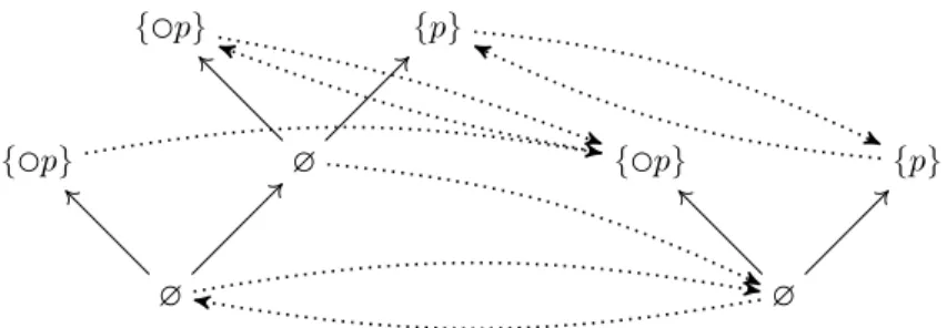
Figure 5: A condensation from the labelled frame on the left to the labelled frame on the right. Dotted arrows indicate the condensation: ρ for arrows from left to right and ι for arrows from right to left.
See Figure 5 for an example of a condensation. Note that the relation≜ is an equivalence relation. In this text, simulations will always be between posets. In the case that A or B is an acyclic directed graph, a simulation between A and B will be one between their respective transitive, reflexive closures. It will typically be convenient to work with immersions rather than simulations: however, as the next lemma shows, not much generality is lost by this restriction.
Lemma 10. Let A=(WA,≼A, λA) and B = (WB,≼B, λB) be labelled posets. If
a simulation σ⊆ WA× WBexists, WA is a finite tree, and w σ w′, then there is
a partial immersion σ′∶ W
A→WB such that w∈ dom(σ′) and w′= σ′(w).
Proof. By a straightforward induction on the depth of w∈ WA we show that if
w σ w′then there is a partial immersion σwwith w∈ dom(σw), whose domain is
the subtree generated by w, and such that σw(w) = w′. Let D be set of daughters
of w, and for each v∈ D, choose v′so that v σ v′and w′≼
Bv′. By the induction
hypothesis, there is a partial immersion σ′
vwith v∈ dom(σv′). Then, one readily
checks that{(w,w′)} ∪ ⋃
v∈Dσv′ is also an immersion, as needed.
Condensations are useful for producing (small) quasimodels out of models. Proposition 7. Given an intuitionistic model M=(WM,≼M, VM), a set Σ ⋐
L◻U, and a ℘(Σ)-labelled poset A = (WA,≼A, λA) over Σ, if A ≪ M, then A is a quasimodel.
Proof. Let(ρ,ι) be a condensation from MΣ
to A. If w≼Av, then ι(w) ≼Mι(v),
so that λA(w) = Σ(ι(w)) ⊆ Σ(ι(v)) = λA(v). Next, suppose that ϕ → ψ ∈ λA(w),
and consider v such that w ≼A v. Then, M, ι(w) ⊧ ϕ → ψ. Since ι is an
immersion, ι(w) ≼Mι(v), hence if M,ι(v) ⊧ ϕ, then also M,ι(v) ⊧ ψ. Thus if
ϕ∈ λA(v), it follows that ψ ∈ λA(v). Finally, suppose that ϕ → ψ ∈ Σ ∖ λA(w).
Then, M, ι(w) ⊭ ϕ → ψ, so that there is v ∈ WM such that ι(w) ≼Mv, M, v ⊧ ϕ
and M, v⊭ ψ. It follows that ϕ ∈ λA(ρ(v)) and ψ /∈ λA(ρ(v)), and since ρ is an
5.3
Normalized labelled trees
In order to count the number of different labelled trees up to bimersion, we construct, for any set Λ of labels and any k ≥ 1, the labelled directed acyclic graph GΛ k =(W Λ k, ↑ Λ k, λ Λ k) by induction on k as follows.
Base case. For k = 1, let GΛ 1 = (W Λ 1 , ↑ Λ 1, λ Λ 1) with W Λ 1 = Λ, ↑ Λ 1= ∅, and λΛ1(w) = w for all w ∈ W Λ 1.
Inductive case. Suppose that GΛ k =(W Λ k , ↑ Λ k, λ Λ
k) has already been defined.
Let us write X∐ Y for the disjoint union of X and Y . The graph GΛ k+1 = (WΛ k+1, ↑ Λ k+1, λ Λ
k+1) is constructed such that:
Wk+1Λ = WkΛ∐ ˜W Λ k+1, where ˜W Λ k+1= Λ × ℘(W Λ k) ↑Λk+1=↑Λk ∪{((ℓ,C),y) ∈ ˜Wk+1Λ × W Λ k ∣ y ∈ C} λΛk+1(w) =⎧⎪⎪⎨⎪⎪ ⎩ λΛk(w) if w ∈ W Λ k ℓ if w=(ℓ,C) ∈ ˜WΛ k+1 Note that GΛ k =(W Λ k, ↑ Λ k, λ Λ
k) is typically not a tree, but we may unravel it
to obtain one.
Definition 11. Given a labelled directed graph G=(W,↑,λ) and w ∈ W, the unravelling of G from w is the labelled tree urw(G) = (urw(W),urw(↑),urw(λ))
such that urw(W) is the set of all the paths in G starting on w, ξ urw(↑) ζ if
and only if there is v∈ W such that ζ = ξv, and urw(λ)(v0. . . vn) = λ(vn).
Proposition 8. For any rooted labelled tree T over a set Λ of labels, if the level of T is finite then there is a condensation from T to ury(GΛlev(T)) for some
y∈ WΛ lev(T).
Proof. Let T=(WT, ↑T, λT) be a labelled tree with root r. We write ≺T for the
transitive closure of ↑T and≼T for the reflexive closure of≺T. The proof is by
induction on the level n= lev(T) of T. For n = 1, observe that this means that λT(w) = λ(r) for all w ∈ WT. Let ρ= WT×{λT(r)} and ι = {(λT(r),r)}. It can
easily be checked that(ρ,ι) is a condensation.2
For n> 1, suppose the property holds for all rooted labelled trees T′such that lev(T′) < n. Define the following sets:
N ={w ∈ WT ∣ λT(w) ≠ λT(r) and for all v ≺ w, λT(v) = λT(r)}
M ={w ∈ W ∣ for all v ≼ w, λT(v) = λT(r)}
Note that if w ∈ N then lev(w) < lev(r), and therefore lev(w) < n; hence by induction, there is a condensation(ρ′
w, ι′w) from the subgraph of T generated
by w to uryw(GΛn−1) for some yw∈ Wn−1Λ .
2Recall that as per our convention, this means that
(ρ, ι) is a condensation between the respective transitive closures.
Define s = (λ(r),{yw∣ w ∈ N}) ∈ WnΛ and consider the unravelling U =
(WU, ↑U, λU) of GΛn from s. Note that uryw(GΛn−1) embeds into U via the map
ξ ↦ sξ, and with this we define ρw∶ WT→WU by ρw= sρ′w, and similarly define
ιw∶ WU → WT by ιw(sξ) = ι′w(ξ) (i.e., ιw first removes the first element of a
string and then applies ι′w).
We then define ρ=(M × {s}) ∪ ⋃ w∈N ρw, ˜ι={(s,r)} ∪ ⋃ w∈N ιw.
Then, it can readily be checked that ρ is an immersion from T to U, ˜ι is a simulation from U to T and ˜ι⊆ ρ−1. Using Lemma 10, we can then choose an
immersion ι⊆ ˜ι, so that (ρ,ι) is a condensation from T to U.
Finally, given n, k∈ N let us recursively define natural numbers En
k and Q n k by: Ekn=⎧⎪⎪⎨⎪⎪ ⎩ 0 if k= 0 En k−1+ n2E n k−1 otherwise Q n k =⎧⎪⎪⎨⎪⎪ ⎩ 0 if k= 0 1+ En k−1Qnk−1 otherwise
The following lemma can be proven by a straightforward induction, left to the reader.
Lemma 11. For any finite set Λ with cardinality n and all k∈ N, 1. the size of GΛ
k is bounded by E n
k, and 2. the size of any unravelling of G Λ
k is bounded by
Qn k.
From this and Proposition 8, we obtain the following:
Theorem 4. 1. Given a set of labels Λ and a Λ-labelled tree T of level k< ω, there is a Λ-labelled tree T′ bounded by Q∣Λ∣k such that T
′≜ T. We call T′
the normalized Λ-labelled tree for T.
2. Given a sequence of Λ-labelled trees T1,⋯, Tn of level k< ω with n > Ek∣Λ∣,
there are indexes i< j ≤ n such that Ti≜ Tj.
Proof. In view of Proposition 8, way may take T to be a suitable unravelling of GΛk, establishing the first claim. For the second, by Lemma 11, GΛk has size at most Ek∣Λ∣. Since the unravellings of any graph are determined by their starting point, there must be i< j ≤ n with Tiand Tj bimersive to the same unravelling
of GΛ
k, from which it follows that Ti and Tj are bimersive.
The second item may be viewed as a finitary variant of Kruskal’s theorem for labelled trees [28]. When applied to quasimodels, we obtain the following: Proposition 9. Let Σ⋐ L◻U with∣Σ∣ = s < ω.
1. Given a tree-like Σ-quasimodel T, there is a tree-like Σ-quasimodel T′≜ΣT
bounded by Q2s
s+1. We call T′the normalized Σ-quasimodel for T.
2. Given a sequence of tree-like Σ-quasimodels T1,⋯, Tn with n> E2 s s+1, there
are indexes i< j ≤ n such that Ti≜ Tj.
Proof. Immediate from Proposition 7 and Theorem 4 using the fact that any Σ-quasimodel has level at most s+ 1.
Finally, we obtain an analogous result for pointed structures.
Definition 12. A pointed labelled poset is a structure (W,≼,λ,w) consisting of a labelled tree with a designated world w ∈ W . Given a labelled poset A = (WA,≼A, λA) and w ∈ WA, we denote by Aw the pointed labelled poset given
by Aw=(W
A,≼A, λA, w). A pointed simulation between pointed labelled posets
A=(WA,≼A, λA, wA) and B = (WB,≼B, λB, wB) is a simulation σ ⊆ WA× WB
such that if w σ v, then w= wA if and only if v= wB. The notions of pointed
immersion, pointed condensation, etc. are defined analogously to Definition 10. Lemma 12. If Λ has n elements, any pointed Λ-labelled poset of level at most k condenses to a labelled pointed tree bounded by Q2n
k+2, and there are at most
E2n
k+2 bimersion classes.
Proof. We may view a pointed labelled poset A=(W,≼,λ,w) as a (non-pointed) labelled poset as follows. Let Λ′ = Λ ×{0,1}. Then, set λ′(v) = (λ(v),0) if
v ≠ w, λ′(w) = (λ(w),1). Note that if A had level k according to λ it may now have level k+ 2 according to λ′, since if u ≺ w ≺ v we may have that
λ(u) = λ(w) = λ(v) yet λ′(u) ≠ λ′(w) and λ′(w) ≠ λ′(v). By Proposition 8, A condenses to a generated tree T of GΛ′
k+2by some condensation (ρ,ι). Let
w′= ρ(w), and consider T as a pointed structure with distinguished point w′. Given that ρ is a surjective, label-preserving function, w, w′ are the only points whose label has second component 1, and therefore (ρ,ι) must be a pointed condensation, as claimed.
With this we may give an analogue of Proposition 9 tailored for pointed quasimodels. Its proof is essentially the same.
Proposition 10. Let Σ⋐ L◻U with ∣Σ∣ = s.
1. Given a tree-like pointed Σ-quasimodel T and a formula ϕ, there is a tree-like pointed Σ-quasimodel T′ ≜ T bounded by Q2s+1
s+3. We call T′ the
normalized pointed Σ-quasimodel for T.
2. Given a sequence of tree-like pointed Σ-quasimodels T1,⋯, Tn with n >
Es+32s+1, there are indexes i< j ≤ n such that Ti≜ Tj.
With these tools at hand, we are ready to prove that ITLe has the effective
6
The Finite Model Property
In view of Proposition 5, in order to show that validity over L is decidable, it suffices to prove that validity is decidable over L◻U. Thus in this section we will
restrict our attention to this sub-language. We will use the notions of eventuality and fulfilment, defined below (see also Figure 6).
Definition 13. Given a model M, an eventuality in M is a pair(w,ϕ), where w∈ W and ϕ is a formula such that either ϕ = ◻ψ for some formula ψ and M, w ⊭ ϕ, or ϕ = ψ U χ for some formulas ψ and χ and M, w ⊧ ϕ. The ful-fillment of an eventuality(w,ϕ) is the finite sequence v0. . . vn of states of the
model such that
1. for all k≤ n, vk= Sk(w),
2. if ϕ= ◻ψ then
(a) M, vn⊭ ψ (the end condition for ϕ) and
(b) for all k< n, M, vk⊧ψ(the progressive condition for ϕ), and
3. if ϕ= ψ U χ then
(a) M, vn⊧χ(the end condition for ϕ) and
(b) for all k< n, M, vk⊧ψ and M, vk ⊭ χ (the progressive condition for
ϕ).
We call n the fulfillment time of(w,ϕ). Given a set of formulas Σ, the fulfill-ment time of w with respect to Σ is the supremum of all fulfillfulfill-ment times of any eventuality (w,ϕ) with ϕ ∈ Σ, and if U is a set of worlds or eventualities, the fulfillment time of U with respect to Σ is the supremum of all fulfillment times with respect to Σ of all elements of U .
The idea is to replace an arbitrary stratified model M by a related model M′ where all eventualities of M′0are realized in effective time. From such a model
M′ we can then extract an effectively bounded finite model Ma←b. The model M′ is a ‘good’ model, defined as follows.
a ⋯ k i ⋯ (w, ϕ) (w′ , ϕ′) ● ● ●● ϕ ●
Figure 6: The stratum Maand two of its eventualities. The fulfillment of(w,ϕ)
Definition 14. Let Σ⋐ L◻U, s=∣Σ∣ and a,b be natural numbers. An expanding
model M is good (with parameters a, b, relative to Σ) if 1. a< b ≤ 2E2n+1 n+1 + Q 2n n+1E 2n+1 n+3, 2. Ma≜ΣMb,
3. Wa has fulfillment time less than b− a, and
4. for all c< b, Mc is bounded by Q2 s+1 s+3.
The bound (1) will naturally arise throughout our construction, but the only relevance is that it is computable. We construct M′ as a speedup of M, in a
sense that we make precise next.
Definition 15. Let Σ⋐ L◻U, M, N be stratified models, and a≤ b′≤ b be natural
numbers. We say that N is a speedup of M from a taking b to b′ if for all i≤ a
Ni= Mi and for all i≥ b′ Ni= Mi+b−b′. We say that N is a strict speedup of
Mif b′< b. We may omit mention of the parameters if we wish to leave them unspecified, e.g. N is a speedup of M from a if there exist b, b′such that N is a
speedup of M from a taking b to b′.
Then, the following speedups are defined for any stratified model M = (W,≼,S,V ) and any finite, non-empty set of formulas Σ closed under subfor-mulas. In each case, if M=(W,≼,S,V ) is a stratified model, we will produce another stratified model M′=(W′,≼′, S′, V′) and a map π∶W′→W such that
ΣM(π(w)) = ΣM′(w) for all w ∈ W′. Below, recall that Mk =(Wk,≼k, Sk, Vk)
denotes the kth
stratum of M.
(su1) Replace Mk with a copy of the normalized Σ-quasimodel of Mk, where
k ≥ 0. Let T = (WT, ↑T, λT) be a copy of the normalized labelled tree
of MΣ
k such that WT∩ W = ∅, and (ρ,ι) the condensation from MΣk to
T. The result of the transformation is the tuple(W′,≼′, S′, V′) such that W′=(W ∖ Wk) ∪ WT,≼′= ≼⇂W∖Wk∪(↑T) ∗ , S′(w) =⎧⎪⎪⎪⎪⎨⎪⎪⎪ ⎪⎩ ρ(S (w)) if w ∈ Wk−1 S(ι(w)) if w ∈ WT S(w) otherwise V′(w) =⎧⎪⎪⎨⎪⎪ ⎩ λT(w) ∩ P if w ∈ WT V(w) otherwise
The map π is the identity on W′
i = Wi for i /= k, and π(w) = ι(w) for
w∈ WT.
(su2) Replace (Mk, w) with a copy of its normalized, pointed Σ-quasimodel,
where k≥ 0 and w ∈ Wk. The transformation is similar to the previous one
except that(Mk, w) is regarded as a pointed structure with distinguished
(su3) Replace Mℓ with Mk, where k< ℓ and there is an immersion σ∶ Wk→Wℓ
(seen as℘(Σ)-labelled trees). The result of the transformation is the tuple (W′,≼′, S′, V′) such that W′= W ∖⋃ k<m≤ℓWm,≼′= ≼⇂W′, S′(w) =⎧⎪⎪⎨⎪⎪ ⎩ S(σ (w)) if S(w) ∈ Wk S(w) otherwise and V′= V ⇂ W′.
The map π is the identity on Wi′= Wi for i< k, on Wi′= Wi+ℓ−k for i> k,
and π(w) = σ(w) for all w ∈ Wk′.
(su4) Replace (Mℓ, wℓ) with (Mk, wk), where k < ℓ, wk∈ Wk, wℓ∈ Wℓand there
is an immersion σ∶ Wk→Wℓ such that σ(wk) = wℓ. The transformation is
defined as the previous one.
Lemma 13. Let a< k < ℓ ≤ b be natural numbers and suppose that M is such that one of the transformations (su1)-(su4) applies. Then, the result M′ is a
speedup of M between a and b such that ΣM(π(w)) = ΣM′(w) for any w ∈ W′.
In the cases (su3) and (su4), the speedup is strict.
Proof. The proof that M′ = (W′,≼′, S′, V′) is a speedup of M = (W,≼,S,V )
consists of checking that Definition 15 applies and is left to the reader. We prove by structural induction on ϕ that for all transformations, all w∈ W′and
all ϕ∈ Σ, M′, w ⊧ ϕiff M, π(w) ⊧ ϕ.
We only detail the case for ϕ= ◯ψ in the sub-case when Mk is replaced with
a copy of the normalized Σ-quasimodel T of Mk and w∈ Wk−1′ . Suppose that
w∈ Wk−1′ and M, π(w) ⊧ ◯ψ. Then ψ ∈ ΣM(Sπ(w)). Since S′(w) = ρSπ(w),
πS′(w) = ιS′(w) and (ρ,ι) is a condensation, ΣM(Sπ(w)) = λT(S′(w)) =
ΣM(πS′(w)). In particular ψ ∈ ΣM(πS′(w)), so that M,πS′(w) ⊧ ψ. By
induction hypothesis, M′, S′(w) ⊧ ψ. Hence M′, w ⊧◯ψ. The other direction
is similar.
The remaining two sub-cases for ϕ = ◯ψ are when w ∈ W′
k and when
w/∈ Wk−1′ ∪ Wk′, both of which are treated similarly. The cases for the other temporal modalities also follow from similar considerations (see also the proof of Lemma 20). The cases for the implication are similar to those in the proof of Proposition 7, and the remaining cases are straightforward. We leave the details to the reader.
The purpose of the transformations (su2) and (su4) is to preserve fulfillments of formulas. We make this precise in the next lemma.
Lemma 14. Let Σ⋐ L◻ U, M= M =(W,≼,S,V ) be a stratified model, a,k ∈ N
with k> 0, and w ∈ Wa. Suppose that ϕ∈ Σ is such that(w,ϕ) is an eventuality
of M with fulfillment w= w0, . . . , wn.
1. If k≤ n and M′is obtained by replacing(M
a+k, wk) by (T,v), then (w,ϕ)
is an eventuality of M′ and the fulfillment of (w,ϕ) is v
0, . . . , vn with
2. If k < ℓ ≤ n and M′ is obtained by replacing (M
a+ℓ, wℓ) by (Ma+k, wk),
then(w,ϕ) is an eventuality of M′and the fulfillment of(w,ϕ) is w0, . . . , wk, wℓ+1, . . . wn.
The proof is straightforward and left to the reader. In the next few lem-mas we show that models can always be sped up so that fulfillment times are effectively bounded.
Lemma 15. Fix Σ⋐ L◻U with s =∣Σ∣ and let M be any startified model and
a< b be natural numbers. Then there is a speedup of M′ of M from a taking b to some b′≤ a + E2s
s+1, and such that M′i is bounded by Q 2s
s+1 for all i∈(a,b′).
Proof. Let b′ be minimal such that some model N is a speedup of M from a
taking b to b′. We claim that b′≤ a + E2s
s+1; for otherwise, by Theorem 4.2 there
are natural numbers i, j with a< i < j ≤ b′such that N
i ≜ΣNj, and hence we
can apply a transformation (su3) to obtain some speedup N′of N from a taking
b′ to some b′′< b′; but then clearly N′ is also a speedup of M from a taking b
to b′′ and b′′< b′, a contradiction.
Thus b′ ≤ a + E2s
s+1, and finally we obtain M′ by replacing each Nx with
x∈(a,b′) by its normalized Σ-quasimodel, which by Proposition 9 is bounded by Q2s
s+1.
Lemma 16. Fix a finite set Σ⋐ L◻U with s=∣Σ∣ and let M = (W,≼,S,V ) be
any stratified model, a∈ N, and U⊆ Wa×Σ be a finite set of eventualities. Then
there is a speedup N of M from a such that the fulfillment time ℓ of U in N satisfies
1. ℓ≤ ∣U∣E2s+1 s+3, and
2. for all x∈ [1,ℓ − a), Na+xis bounded by Q2 s+1 s+3.
Proof. By induction on∣U∣. The claim is vacuously true if U = ∅. Otherwise, let n+ 1 =∣U∣ and (w,ϕ) ∈ U and assume inductively that a speedup M′of M
from a is given so that the fulfilment time of U∖{(w,ϕ)} in M′ is ℓ≤ nE2s+1 s+3
and for all x< ℓ − a, Na+1+x is bounded by Q2 s+1 s+3.
Let N be a speedup of M′from a+ ℓ chosen so that the fulfilment time r of
(w,ϕ) in N is least among all such speedups. We claim that r ≤ (n + 1)E2s+1 s+3.
If not, let w0, . . . , wr be the fulfilment path for (w,ϕ), and for x ∈ [1,r − ℓ]
let N+
ℓ+x be the pointed submodel (Nℓ+x, wℓ+x). Note that r − ℓ > E2 s+1 s+3 , so
that by Proposition 10 there are x, y ∈ N such that 0 < x < y ≤ r − ℓ and N+ℓ+x≜ΣN+ℓ+y. Thus we can apply a transformation (su4) and replace N+ℓ+y by
N+ℓ+x to obtain a speedup N′ of N. By Lemma 14, the fulfilment of (w,ϕ) in N′is w0, . . . , wℓ+x, wℓ+y+1, . . . , wr, so that(w,ϕ) has fulfilment time r − (y − x), contradicting the minimality of r.
Finally we define N′ by replacing each (Nℓ+x, wℓ+x) with x ∈ [0,r − ℓ) by
its pointed, normalized Σ-quasimodel, which in view of Proposition 10 has size at most Q2s+1
s+3 and by Lemma 14 preserves the fulfilment time of (w,ϕ), as
In the next lemmas we construct a good model in three phases, each time obtaining more of the properties required by Definition 14. Below, if Σ⋐ L◻U
and M=(W,≼,S,V ) is a stratified model and a ∈ N, we say that Ma occurs
infinitely often (with respect to Σ) if there are infinitely many values of i such that Ma≜ΣMi.
Lemma 17. Let Σ⋐ L◻ U and s = ∣Σ∣ and ϕ ∈ Σ. Then ϕ is satisfiable
(fal-sifiable) over the class of expanding posets if and only if ϕ is satisfied in an expanding model M for which there exists a≤ E2s
s+1 such that
1. Ma occurs infinitely often and
2. for all i≤ a the size of Mi is bounded by Q2 s s+1.
Proof. Suppose that ϕ is satisfiable (falsifiable). Then, by Theorem 1, ϕ is satisfied (falsified) on N0 for some stratified model N. By Proposition 9 there
are finitely many≜Σ equivalence classes, and hence there is some a′ such that
Na′ occurs infinitely often.
By Lemma 15 there is a speedup M′of N from 0 taking a′to some a≤ E2s s+1
and such that the size of M′iis bounded by Q 2s
s+1for all i∈(0,a). It is then easy
to see that M′a occurs infinitely often in M′. Finally we define M by replacing
M′0 and M′a by their normalized ℘(Σ)-labelled trees, which by Proposition 9 have size at most Q2s
s+1.
Lemma 18. Let Σ⋐ L◻U with s=∣Σ∣ and ϕ ∈ Σ. Then ϕ is satisfiable
(falsifi-able) over the class of dynamic posets if and only if ϕ is satisfied in a stratified model M for which there exists a≤ E2s
s+1 such that
1. Ma occurs infinitely often,
2. Wa has fulfilment time r≤ sQ2 s s+1E
2s+1 s+3, and
3. for all i≤ a + r, Mi is bounded by Q2 s+1 s+3.
Proof. In view of Lemma 17, we may assume that ϕ is satisfied (falsified) on N0for some expanding model N=(W,≼,S,V ) satisfying the first condition and
such that for all i≤ a the size of Mi is bounded by Q2 s
s+1. Let U ⊆ Wa× Σ be
the set of all eventualities of Na; by Lemma 16 there is a speedup M′ of N
from a such that the realization time of M′
a is bounded by ∣U∣E 2s+1 s+3 and such that M′ a+1+i is bounded by Q 2s+1
s+3 for all i < r. Clearly ∣U∣ ≤ s∣Wa∣ ≤ sQ2 s s+1,
giving us the second condition. Since for i≤ a we have that Mi is bounded by
Q2s s+1≤ Q
2s+1
s+3, we obtain the third condition.
Finally we are able to show that satisfiability and validity can be restricted to good models.
Lemma 19. Let Σ⋐ L◻U with s=∣Σ∣ and ϕ ∈ Σ. Then ϕ is satisfiable
(falsifi-able) over the class of expanding posets if and only if ϕ is satisfied (falsified) in a good model.
Proof. We may begin with a model N=(W,≼,S,V ) satisfying all conditions of Lemma 18, where Na occurs infinitely often and r is the realization time of Wa.
Since Ma occurs infinitely often, we may choose b′> a + r such that Na≜ΣNb′.
Then, by Lemma 15 there is a speedup M of N from a+ r taking b′ to some
b≤ a + r + Es+12s+1 and such that Miis bounded by Q2 s+1
s+1 (and hence by Q 2s+1 s+3) for
all i∈(a + r,b). The model M then has all desired properties.
Definition 16. Let M be an expanding model such that there is an immer-sion σ∶ Wb → Wa. Then we define a new pointed model Ma←b = (Wa←b,≼a←b
, Sa←b, Va←b, wa←b0 ) by setting Wa←b=⋃0≤m<bWm,≼a←b= ≼⇂Wa←b,
Sa←b(w) =⎧⎪⎪⎨⎪⎪ ⎩
σ(S (w)) if w ∈ Wb−1
S(w) otherwise
Va←b= V ⇂Wa←b, and w0a←b to be the root of W0 (note that wa←b0 ∈ Wa←b).
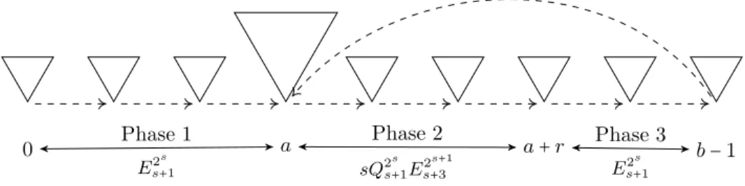
The idea is to apply the operation ⋅a←b to good models, in which case the end result is a well-behaved finite model as described in the next lemma and Figure 7. 0 Phase 1 a a + r b −1 E2 s s+1 Phase 2 sQ2 s s+1Es+32s+1 Phase 3 E2s s+1
Figure 7: An illustration of the three phases of Ma←b built from a good model.
Below each phase we indicate the maximum number of strata, used for the computations in the proof of Lemma 21.
Lemma 20. If M = (W,≼,S,V ) is a good model with parameters a, b then Ma←b is a model and ΣMa←b(w) = ΣM(w) for all w ∈ Wa←b.
Proof. The proof that Ma←b=(Wa←b,≼a←b, Sa←b, Va←b) is a model is
straight-forward and left to the reader. We prove by structural induction on ϕ that for all w∈ Wa←b and all ϕ∈ Σ, Ma←b, w ⊧ ϕ iff M, w ⊧ ϕ. The cases for
proposi-tional variables and the Boolean connectives are straightforward. The case for the ‘next’ temporal modality is similar to that in the proof of Lemma 13.
For the ‘henceforth’ and ‘until’ temporal modalities, suppose first that(w,ϕ) is an eventuality in M and w∈ Wa←b. Let w
0. . . wn be the fulfilment of(w,ϕ)
in M. If wn∈ Wa←bthen we can apply the induction hypothesis to see that each