Adaptation response surfaces for managing wheat under perturbed climate and CO
2
in
a Mediterranean environment
M. Ruiz-Ramos
a,⁎
, R. Ferrise
b, A. Rodríguez
a, I.J. Lorite
c, M. Bindi
b, T.R. Carter
d, S. Fronzek
d, T. Palosuo
e,
N. Pirttioja
d, P. Baranowski
f, S. Buis
g, D. Cammarano
h, Y. Chen
e, B. Dumont
i, F. Ewert
j, T. Gaiser
j,
P. Hlavinka
k,l, H. Hoffmann
j, J.G. Höhn
e, F. Jurecka
k,l, K.C. Kersebaum
m, J. Krzyszczak
f, M. Lana
m,
A. Mechiche-Alami
n, J. Minet
o, M. Montesino
p, C. Nendel
m, J.R. Porter
p, F. Ruget
h, M.A. Semenov
q,
Z. Steinmetz
r, P. Stratonovitch
q, I. Supit
s, F. Tao
e, M. Trnka
k,l, A. de Wit
s, R.P. Rötter
taUniversidad Politécnica de Madrid, ETSIAAB, 28040 Madrid, Spain b
University of Florence, 50144 Florence, Italy
c
IFAPA Junta de Andalucía, 14004 Córdoba, Spain
d
Finnish Environment Institute (SYKE), 00250 Helsinki, Finland
e
Natural Resources Institute Finland (Luke), 00790 Helsinki, Finland
fInstitute of Agrophysics, Polish Academy of Sciences, Doświadczalna 4, 20-290 Lublin, Poland gINRA, UMR 1114 EMMAH, F-84914 Avignon, France
hJames Hutton Institute, Invergowrie, Dundee DD2 5DA, Scotland, United Kingdom i
Dpt. AgroBioChem & Terra, Crop Science Unit, ULgGembloux Agro-Bio Tech, 5030 Gembloux, Belgium
j
INRES, University of Bonn, 53115 Bonn, Germany
k
Institute of Agrosystems and Bioclimatology, Mendel University in Brno, Brno 613 00, Czech Republic
l
Global Change Research Institute CAS, 603 00 Brno, Czech Republic
mInstitute of Landscape Systems Analysis, Leibniz Centre for Agricultural Landscape Research (ZALF), 15374 Müncheberg, Germany nDepartment of Physical Geography and Ecosystem Science, Lund University, 223 62 Lund, Sweden
o
Université de Liège, Arlon Campus Environnement, 6700 Arlon, Belgium
p
University of Copenhagen, 2630 Taastrup, Denmark
q
Rothamsted Research, Harpenden, Herts AL5 2JQ, UK
r
RIFCON GmbH, 69493 Hirschberg, Germany
s
Wageningen University, 6700AA Wageningen, The Netherlands
tTROPAGS, Department of Crop Sciences, Georg-August-Universität Göttingen, Grisebachstr. 6, 37077 Göttingen, Germany
a b s t r a c t
a r t i c l e i n f o
Article history:
Received 27 September 2016
Received in revised form 12 January 2017 Accepted 16 January 2017
Available online xxxx
Adaptation of crops to climate change has to be addressed locally due to the variability of soil, climate and the specific socio-economic settings influencing farm management decisions. Adaptation of rainfed cropping sys-tems in the Mediterranean is especially challenging due to the projected decline in precipitation in the coming decades, which will increase the risk of droughts. Methods that can help explore uncertainties in climate projec-tions and crop modelling, such as impact response surfaces (IRSs) and ensemble modelling, can then be valuable for identifying effective adaptations. Here, an ensemble of 17 crop models was used to simulate a total of 54 ad-aptation options for rainfed winter wheat (Triticum aestivum) at Lleida (NE Spain). To support the ensemble building, an ex post quality check of model simulations based on several criteria was performed. Those criteria were based on the“According to Our Current Knowledge” (AOCK) concept, which has been formalized here. Ad-aptations were based on changes in cultivars and management regarding phenology, vernalization, sowing date and irrigation. The effects of adaptation options under changed precipitation (P), temperature (T), [CO2] and soil type were analysed by constructing response surfaces, which we termed, in accordance with their specific pur-pose, adaptation response surfaces (ARSs). These were created to assess the effect of adaptations through a range of plausible P, T and [CO2] perturbations. The results indicated that impacts of altered climate were pre-dominantly negative. No single adaptation was capable of overcoming the detrimental effect of the complex in-teractions imposed by the P, T and [CO2] perturbations except for supplementary irrigation (sI), which reduced the potential impacts under most of the perturbations. Yet, a combination of adaptations for dealing with climate change demonstrated that effective adaptation is possible at Lleida. Combinations based on a cultivar without vernalization requirements showed good and wide adaptation potential. Few combined adaptation options Keywords:
Wheat adaptation Sensitivity analysis Crop model ensemble Rainfed
Mediterranean cropping system AOCK concept
Agricultural Systems xxx (2017) xxx–xxx
⁎ Corresponding author.
E-mail address:[email protected](M. Ruiz-Ramos).
http://dx.doi.org/10.1016/j.agsy.2017.01.009
0308-521X/© 2017 Elsevier Ltd. All rights reserved.
Contents lists available atScienceDirect
Agricultural Systems
performed well under rainfed conditions. However, a single sI was sufficient to develop a high adaptation poten-tial, including options mainly based on spring wheat, current cycle duration and early sowing date. Depending on local environment (e.g. soil type), many of these adaptations can maintain current yield levels under moderate changes in T and P, and some also under strong changes. We conclude that ARSs can offer a useful tool for supporting planning offield level adaptation under conditions of high uncertainty.
© 2017 Elsevier Ltd. All rights reserved.
1. Introduction
The Mediterranean basin has been identified as one of the most prom-inent climate change hotspots due to ongoing and projected changes in both means and variability of temperature and precipitation (Diffenbaugh and Giorgi, 2012). Observed climate showed a trend to-wards increasing temperature and declining rainfall over recent decades (Hartmann et al., 2013, Figs. 2.22 and 2.29). This trend is estimated to con-tinue over the 21st century, with multi-model median projections show-ing reduced annual precipitation (ca.−15% of projected mean change, with high uncertainty) and increased mean annual temperature (ca. +5 °C) by the end of the century under the highest scenario of radiative forcing of the atmosphere (8.5 W m−2) simulated by climate models (RCP8.5;IPCC, 2013). Associated with these changes is a projected in-crease in the frequency and intensity of extreme daily maximum temper-atures (Collins et al., 2013;Sánchez et al., 2004, for the Iberian Peninsula). In turn, climate change is estimated to generate severe impacts on agricul-ture, constituting an important risk to food production (Asseng et al., 2015). These impacts are mainly driven by drought and heat stress. Spe-cifically for wheat (Triticum aestivum), the majority of the impacts are driven by temperature (Tack et al., 2015) rather than precipitation, resulting in significant yield reduction with temperature increases (Asseng et al., 2015). However, high-temperature episodes might have larger negative effects under water stress conditions, which are very fre-quent in the Mediterranean region (e.g.Moriondo et al., 2010). The posi-tive effects of increasing [CO2] do not completely counteract this trend
(Ferrise et al., 2011). The wheat yield stagnation detected in several re-gions during recent decades (Grassini et al., 2013) could be thefirst evi-dence of these effects.
Specifically for winter wheat in Spain,Olesen et al. (2007)projected a mean yield decrease of 21% by the end of the 21st century, and
Mínguez et al. (2007)revealed a northward shift of winter wheat failure due to disturbed vernalization (i.e. when cold requirements for normal flowering induction are not met due to higher temperatures).Mínguez et al. (2007)also projected a variable yield response in northern Spain, with yield decreases linked to low elevation areas and increases to higher elevation. Also for Spain,Iglesias et al. (2010)concluded that de-creases in cereal yields would be less severe in northern parts of Spain than in southern parts. Taken together, this evidence for substantial im-pacts of climate change on winter wheat cultivated under current prac-tices in the Mediterranean basin, points to a clear need to examine options for adaptation.
To identify optimal adaptation strategies, the quantification of com-plex crop–climate–soil interactions and phenology analysis is essential (Rötter et al., 2011; Wang et al., 2015). Current research is exploring strategies to deal with heat and water stress by modifying crop varieties and management according to the environment, optimizing the Geno-type × Management × Environment (G × M × E) interaction (Montesino-San Martin et al., 2015; Rötter et al., 2015).
The development of new heat-tolerant cultivars has been recom-mended (Olesen et al., 2011; Semenov et al., 2014; Tanaka et al., 2015) to deal with the projected changes in both mean climate condi-tions and occurrence of extreme events during sensitive periods of the crop cycle (Moriondo et al., 2011; Ruiz-Ramos et al., 2011). Other rec-ommendations include changes in cycle duration, seeking a better match of phenology with future local climate (Semenov et al., 2014). Specifically for Spain and winter wheat, the shortening of the crop
cycle has been suggested as an adaptation option, in particular when considering the effect of heat stress (Moriondo et al., 2011). Also, where higher temperatures trigger an increase of development rate, longer cycles could show adaptation potential (Giannakopoulos et al., 2009). Other potential cultivar characteristics, desirable for both current and future cultivars, could include increased water use efficiency and the ability to exploit high [CO2] (O'Leary et al., 2015). Removal of
vernal-ization requirements is also a promising strategy, as indicated by the positive impacts reported for spring wheat due to milder temperatures in Spain under future conditions. This effect was more evident in north-ern Spain (the region where the winter wheat currently meets vnorth-ernali- vernali-zation requirements), as current winter temperatures limit crop growth (Mínguez et al., 2007).
Regarding management, researchers are proposing the adoption of early sowing dates for many European regions (Olesen et al., 2011) and specifically for Spain and winter wheat (Giannakopoulos et al., 2009; Moriondo et al., 2010). Also, water management optimization under rainfed (Olesen et al., 2011) or irrigated cultivation has been suggested, as well as the expansion of irrigation infrastructure (Tanaka et al., 2015), and an increased intensity of both the cropping system and the ir-rigation system (Mínguez et al., 2007;Moriondo et al. (2010), although the latter might be precluded in Spain due to future competition for water resources among agriculture and other sectors. The ultimate goal of these techniques is not only to increase but also to stabilize yields.
A single adaptation option might not be enough to cope with climate change impacts in a Mediterranean climate. Results for Spain indicate that combined adaptation measures ameliorate yield declines better than single ones, and in some cases are capable of maintaining current yields (e.g.Rey et al., 2011). For example,Gabaldón-Leal et al. (2015)
simulated yield responses to a combination of adjustments in sowing date, growth duration, phyllochron, grainfilling rate and water use effi-ciency for irrigated maize in Spain.
In practice, there are trade-offs between the outcomes of individual adaptations, which can complicate the implementation of potential ad-aptation measures. For example, under dry conditions early maturity helps a crop to avoid excessive water stress but also results in lower yields due to a shorter crop cycle (Semenov et al., 2014). In turn, these trade-offs will depend on site-specific conditions and the particular combination of adaptations selected. In this complex context, re-searchers, technicians and farmers require the development of locally tailored adaptation strategies (Reidsma et al., 2015) according to the magnitude and features of the projected regional climate change, soil type, and economic analyses of favourable management options (e.g. for different water prices,Rey et al., 2011).
Besides practical implementation, the modelling of adaptation is also challenging because of multiple sources of uncertainty (Iglesias et al., 2010). There can be large discrepancies between simulated and measured results (O'Leary et al., 2015), and wheat model sensitivities to climate can also differ substantially (Pirttioja et al., 2015; Ruane et al., 2016). Thus, in spite of the recent improvements in modelling, there are still challenges in simulating processes affecting responses in phenology, water use ef fi-ciency or harvest index, even under current climate conditions. These un-certainties can be exacerbated under higher temperatures outside the range of historical experience (Asseng et al., 2015).
Crop models, usually based on ecophysiological knowledge and draw-ing, to a varied extent, on empirical relationships, have been proven to be useful tools to simulate G x M x E interactions for both deepening our
understanding of crop behaviour and also facilitating application in stud-ies of crop response (Montesino-San Martin et al., 2015; Rötter et al., 2015). Moreover, crop model ensembles can provide a powerful tool for combining the responses of various crop simulation models. This can pro-vide useful insights on inter-model uncertainties in yield responses. It can also help to identify robust behaviour across models, both in terms of av-erage responses (e.g. see the multi-model sensitivity study byPirttioja et al. (2015)that utilizes impact response surfaces) as well as sensitivity to interannual climate variability (Ruane et al., 2016). No model reproduces observations perfectly under different environments (e.g.Palosuo et al., 2011) and some authors claim that multi-model ensemble-average esti-mates are more accurate than estiesti-mates from any single model in simu-lating yield responses to climate change (Asseng et al., 2015), with improved accuracy as ensemble size increases up to a certain number of ensemble members beyond which improvements become negligible (Martre et al., 2015).
The objective of this paper is to analyse yield response to changes in mean climatic conditions, as well as to explore options for effective local adaptation of wheat in the Mediterranean under highly uncertain fu-ture. For this purpose, we used an ensemble of 17 crop simulation models to calculate wheat yield responses in Lleida, Spain, through a range of possible climate perturbations with various adaptation options. Impact response surfaces (IRSs) were used in the analysis, and we have developed the concept of adaptation response surfaces (ARSs) to sup-port the analysis of adaptation.
2. Material and methods
2.1. Study site, experimental data and climate data
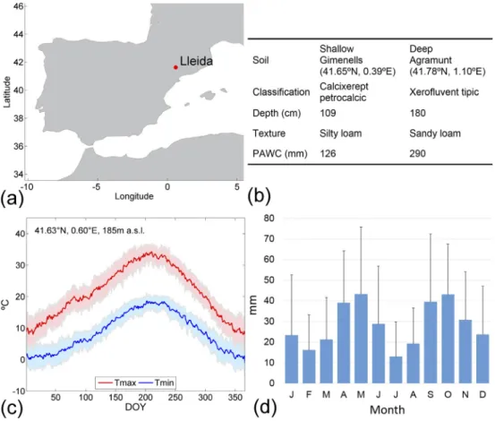
The study was conducted at Lleida in northeastern Spain, one loca-tion representative of the wheat cultivaloca-tion area in the“Mediterranean
South” environmental zone (Metzger et al., 2005,Fig. 1a). The principal characteristics and agro-climatic conditions of Lleida are summarized in
Fig. 1b, c, d.
Modellers were provided with phenological observations (flowering and maturity dates), total above-ground biomass, average grain weights and yields for the winter wheat variety Soissons. Thesefield data were taken fromAbeledo et al. (2008)andCartelle et al. (2006)and were ba-sically the same as those used byPirttioja et al. (2015). The data includ-ed three irrigatinclud-ed treatments and one for rainfinclud-ed, four N management treatments and six sowing dates (spanning from November to Febru-ary), and comprised two locations close to each other in Lleida province (Agramunt and Gimenells) and two growing seasons (2003–2004 and 2005–2006). Statistical data for Lleida province means from Spanish Ministry of Agriculture were used to check interannual variability for the period 1980–2010. Two representative actual soil profiles from these locations, exhibiting contrasting soil depth and texture and there-fore water holding capacity were considered in the study (Fig. 1b).
Weather data from micrometeorological weather stations located in thefield experiments were considered for model calibration. For the simulation phase (described inSection 2.2.3), the baseline climate was taken from the AEMET weather station at Lleida during the period 1980–2010. These baseline data were then perturbed to conduct a sen-sitivity analysis of the crop models to changes in climate. All datasets were at a daily time step for global solar radiation, minimum and max-imum temperature (Tmin, Tmax), precipitation (P), wind speed and rel-ative humidity. Missing values were derived from ERA-Interim reanalysis as described inPirttioja et al. (2015). To create the perturbed dataset, P and temperature (T) baseline values were systematically modified using a “change factor” approach in combination with a sea-sonal pattern of the T and P changes (Fronzek et al., 2010). Observed daily Tmax and Tmin were modified between −1 °C and +7 °C at 1 °C intervals. Daily P was modified between −40% and +30% at 10%
Fig. 1. Location of the study site (a). Main features of the soils considered in the simulation phase (b). Long-term (1981–2010) mean daily minimum (Tmin) and maximum (Tmax) temperature with standard deviation (SD) as shadow areas (c) and monthly precipitation with SD as error bars (d) at the Lleida weather station.
intervals. These ranges were set to encompass uncertainties in projected climate changes at Lleida by the middle of the 21st century for the medium SRES A1B emissions scenario. These uncertainties com-bine information from observations and from climate models, speci fi-cally multi-model ensemble results from the Coupled Model Intercomparison Project phase 3 (CMIP3) and perturbed physics en-sembles (Harris et al., 2010), and are also consistent with regional pro-jections for the highest implied emissions (RCP8.5) from the multi-model ensemble CMIP5 data sets (Collins et al., 2013). Thus, each year of the baseline was modified according to 72 combinations of perturbed T and P. To account for differences in the treatment of air humidity by crop models, vapour pressure and dew point temperature were corrected for temperature changes by assuming relative humidity to re-main unchanged. The introduction of the seasonal pattern consisted of applying seasonal weights to the baseline climate instead of constant T and P changes over all days of the year, while retaining the annual mean changes (Fronzek et al., 2010). The seasonal weights were calcu-lated from the ensemble mean of the Hadley Centre probabilistic cli-mate change projection based on the A1B emissions scenario (Harris et al., 2010).
2.2. Crop modelling
2.2.1. Crop models and calibration guidelines
An ensemble of 17 members made up of 14 wheat models and 17 modelling groups was applied in this study (listed in Table S1 in Suppl. mat.). All the models used in this study have been applied suc-cessfully over a range of regions and applications (references in
Rosenzweig et al., 2013; examples of ensemble modellingAsseng et al., 2015; Martre et al., 2015; Pirttioja et al., 2015;Palosuo et al., 2011). The same model/version was contributed separately byfive modelling groups for two models (2 × CERES-wheat and 3 × WOFOST) and they were considered as separate models followingPirttioja et al. (2015). An overview of all crop models and their differences in terms of main process representation is provided inPirttioja et al. (2015). Most of the models were developed for thefield scale, except for CARAIB, LPJ and MCWLA, which were developed for larger area model-ling. All models operate on a daily time step.
Modellers were asked to calibrate their model using the experimen-tal data provided that included a diversity of treatments to represent the crop cultivation in the study area (seeSection 2.1) and assuming [CO2]
to be 360 ppm. The calibration was donefirst for parameters affecting phenology and thereafter for parameters affecting crop growth and yield. The specific formulation of these parameters varied among models. The modellers were left free to use the calibration method they preferred (e.g. trial and error or automatic), but they were asked to check that calibration performance was within the“good” category according toJamieson et al. (1991). This corresponds to a normalized root mean square error between simulated and observed values lower than 20%.
2.2.2. Preliminary study to identify potential adaptations
To save the workload of modellers, two crop models, CERES-wheat (Jones et al., 2003) DSSATv4.5 and SiriusQuality2 (SQ2) (Martre et al., 2006) were selected to explore and narrow the wide range of possible adaptations, and to identify the most promising ones to be simulated by all the participants. This was necessary due to the huge number of possible adaptation options that result just from combining some of the most important options, such as changes in crop phenology, sowing dates and water management.
Thus, two types of phenological change were tested: changes in the vernalization requirements (Mínguez et al., 2007) and changes in the length of the phenological phases. In the study region spring wheat spans the same sowing dates as winter wheat; sowing date in turn de-pends on autumn rain, so switching between spring- and winter-type cultivars is already possible. Both shorter and longer growth cycles
were proposed; the shorter cycles could provide beneficial if they re-duce the risk of encountering adverse weather events (Trnka et al., 2014) while longer cycles would benefit from a prolonged period of photosynthesis and grainfilling (Olesen et al., 2007; Trnka et al., 2014). Both reduced and extended growth cycles are regarded as feasi-ble options by agronomy experts (Olesen et al., 2011).
Changes in sowing dates were also explored: advancing sowing date increases crop growth cycle length, moves the cycle towards a cooler part of year and helps the crop to avoid the stressful conditions at the end of the cycle (Ferrise et al., 2011; Olesen et al., 2007). However such advancement is constrained by the end of the dry season, projected to last longer on the Iberian Peninsula in the future (Trnka et al., 2014). A delayed sowing date moves the crop cycle towards the most effective period for fulfilling the vernalization requirements (Moriondo et al., 2011) and closer to the winter precipitation (Ruiz-Ramos and Mínguez, 2010).
Supplementary irrigation (sI) at sensitive crop growth stages is a means to stabilize yields, and is already being explored for many crops in Spain and in other Mediterranean countries (Lorite et al., 2012).
Table 1summarizes the options (single and combined) tested for iden-tification of adaptations.
2.2.3. Simulation phase
Afirst set of model runs consisted of simulations without consider-ation of adaptconsider-ation measures, i.e. standard simulconsider-ations. We define stan-dard simulations as those with the winter wheat stanstan-dard cultivar; crop cycle and stages defined as in the calibration process (Section 2.2.1) and standard management, i.e. sowing date set at day of year (DOY) 302, no irrigation but no other limiting factors. A second set of model runs consisting of a limited set of promising single and combined adaptation options were selected in the preliminary phase and simulated by all par-ticipants. A full irrigation (fI) scenario, simulating crop growth without any water stress, also served as a reference for identifying yield ceilings and associated water requirements.
The sensitivity analysis of crop response to climate change was per-formed by following the general procedure described in, for example,
Martre et al. (2015)andPirttioja et al. (2015). The period 1981–2010 was used as the baseline. Models were applied under the 72 combina-tions of perturbed weather described inSection 2.1and with two soil profiles (Fig. 1b). Simulations were performed as a series of indepen-dent growing seasons with initial soil water content set at 75% offield capacity at the beginning of the season. Two levels of [CO2] representing
two 20-year time slices for periods centred on 2030 and 2050 according to A1B projections from the BernCC model (Nakicenovic and Swart, 2000) were considered. Additionally, the standard simulations were performed with [CO2] at 360 ppm as a baseline level.
2.3. Analysis of results
IRSs are plotted surfaces that show the response of an impact vari-able to changes in two explanatory varivari-ables (here, P and T). They are constructed by plotting the results of the sensitivity analysis of model outputs as contour lines along the axes of P and T changes (Fronzek et al., 2010; Pirttioja et al., 2015). Contour lines were computed with the statistical software environment R (http://www.R-project.org/). Indi-vidual IRSs of the 30-year mean yield were generated for each crop model and standard management and cultivar or adaptation option. Yield estimates across multiple models were averaged using the ensem-ble median to be consistent with previous studies (e.g.Asseng et al., 2015; Pirttioja et al., 2015). The utility of IRS analyses for displaying how crop models differ in their sensitivity to systematic changes in input variables such as T and P has been demonstrated in earlier studies (Ferrise et al., 2011; Pirttioja et al., 2015).
In order to analyse the effect of an adaptation option under combina-tions of T and P change, IRSs were constructed both with and without the given adaptation option and for the same [CO2] and then the
difference between the two was calculated. We refer to this new plot as an Adaptation Response Surface (ARS– illustrated inFig. 2). In this con-text, the isolines of the ARS can be expressed as an absolute value or as a percentage (as inFig. 2). Baseline 30-year mean yields (i.e. of the unper-turbed simulation) were considered together with the ARSs to evaluate the ability of different adaptation options to maintain current yield levels, labelled here as the“recovery response”. This was done by superimposing a mask on the Adapted IRSs and the corresponding ARSs using the current yield as threshold (colour mask inFig. 2). Current yield was calculated as the multi-model median of 30-year mean yields at unperturbed P and T under 360 ppm and with no adaptation for each soil type. It is important to stress that the ARS isolines refer to the adap-tation response as defined above, and not to the recovery response.
Inter-annual variability of yield was expressed as the ensemble me-dian of the coefficients of variation (CVs) across the 30 years for each model. The spread in model responses was evaluated by the inter-quar-tile range of the 30-year mean (IQR, from the 25th to the 75th percentile).
It has been suggested that multi-member ensembles of crop simula-tion models generate more robust results in projecting impacts of cli-mate change (Asseng et al., 2015; Martre et al., 2015; Palosuo et al., 2011). In our study, slightly different ensembles were used for the var-ious adaptation options. This was because the construction of the en-sembles was co-determined by the fact that some models did not simulate all the options, summarized in Table S1. Besides, we excluded all the simulations with technical errors and those with very evidently unrealistic model response or absolute values of simulated variables after one-round of discussion with the modellers and based on the
authors' expert judgment and referred to here as“According to Our Cur-rent Knowledge” (AOCK). In that way, the simulations were checked for some highly implausible ecophysiological responses. Thus, for model simulations assuming standard management and cultivar, if one or more of the AOCK-defined criteria were met by the 30-year mean of an output variable, the simulation was excluded. For these criteria, thresholds were set supported by the literature and/or AOCK. Given the subjective nature of this exercise the thresholds were set sufficiently wide to ensure that plausible results were not excluded from the en-sembles. The criteria were as follows:
• yields were higher than 10.5 t ha−1under rainfed conditions for
unper-turbed P and T, which is ca. 3 t (40%) higher than the maximum yield observed from irrigated treatments (Abeledo et al., 2008). • yields were higher for the shallow soil than for the deep soil when all
other settings were the same for unperturbed P and T, which is highly implausible in a water stressed environment, given that deep soils can hold more water.
• yields were the same for rainfed and irrigated simulations for unper-turbed P and T, whereasfield data show clear benefits from irrigation. • yields were higher for rainfed compared to irrigated at unperturbed P and increased T, when the simulated length of the cycle and all other condi-tions were the same. This is very unlikely as, given all other condicondi-tions are identical, rainfed yields limited by water availability should always be lower or maximum the same as yields of full irrigated crops that do not experience water stress.
• the yield change was independent of P under rainfed conditions, i.e. less than 5% of change in yield from−40% to +40% of P change, whereas
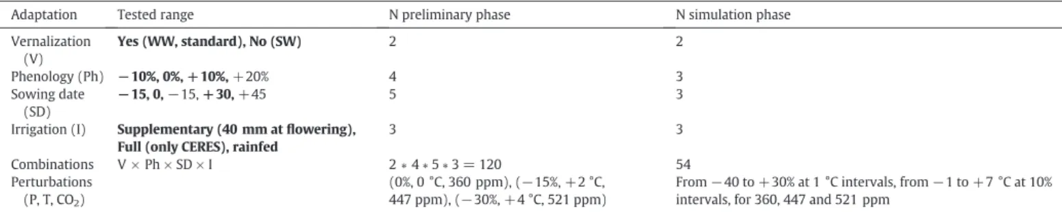
Table 1
Adaptation options and climate/[CO2] perturbations tested in the preliminary phase (normal font) and selected for the simulation phase (bold font). Simulations of the preliminary phase
were run with CERES-wheat and SiriusQuality2 models.
Adaptation Tested range N preliminary phase N simulation phase
Vernalization (V) Yes (WW, standard), No (SW) 2 2 Phenology (Ph) −10%, 0%, +10%, +20% 4 3 Sowing date (SD) −15, 0, −15, +30, +45 5 3
Irrigation (I) Supplementary (40 mm atflowering), Full (only CERES), rainfed
3 3 Combinations V × Ph × SD × I 2∗ 4 ∗ 5 ∗ 3 = 120 54 Perturbations (P, T, CO2) (0%, 0 °C, 360 ppm), (−15%, +2 °C, 447 ppm), (−30%, +4 °C, 521 ppm)
From−40 to +30% at 1 °C intervals, from −1 to +7 °C at 10% intervals, for 360, 447 and 521 ppm
Abbreviations: winter wheat (WW), spring wheat (SW), temperature (T), precipitation (P).
Fig. 2. Example of adaptation response surface (ARS) construction. An ARS results from subtracting two impact response surfaces (IRSs): one considering the adaptation to be evaluated (here using spring wheat), and the other the standard, unadapted option. In this case, the isolines of yield in the IRSs are in kg ha−1, while the results in the ARS are expressed as % of change
from the unadapted option. Both IRSs correspond to the same [CO2] (here 447 ppm) and the same soil (here the shallow soil); therefore, only the effect of the adaptation is evaluated. The
green and red mask separates respective yields above and below a reference yield, defined as the baseline 30-year mean yield at unperturbed P and T under 360 ppm for a given soil type without any adaptation (here 5100 kg ha−1). (For interpretation of the references to colour in thisfigure legend, the reader is referred to the web version of this article.)
field data show a clear sensitivity to precipitation.
• the simulated crop cycle was too short for both standard and adapted cul-tivars. Warming is known to accelerate phenological development of crops, but it is unrealistic for crop cycle to be excessively reduced. Threshold for earliest end of cycle at maturity defined here was 1st of April when checked up to +2 °C. This is 2 months earlier than cur-rent observed dates in the South of Spain with mean annual temper-ature ca. 2 °C warmer than Lleida - data fromwww.aemet.es.
3. Results
3.1. Crop model calibration
Normalized RMSEs for the simulated anthesis and maturity dates for the ensemble of models were 3.8% and 3.2% respectively (corresponding to a mean error of 5.8 and 5.8 days respectively). Normalized RMSEs for the simulated yield and biomass for the ensemble of models were 14.6% and 9.6%. Normalized RMSE for all these variables for each individual model was always below 20% for biomass and yield and up to 5% for an-thesis and maturity dates (see Table S2 in Suppl. mat. for individual model results). Although the observed data set is referred only to two years this can be compensated by the wide variability of treatments considered. Besides, we checked that the ensemble members and the ensemble median were generally able to reproduce the interannual var-iability for the 1980–2010 period (Fig. S1). Therefore, according to
Jamieson et al. (1991), we considered all the models acceptable for this specific application at this location.
3.2. Preliminary phase
Simulated yields for the adaptations tested in the preliminary phase are reported inTable 2.Table 2illustrates the actual situation in crop modelling, when models show opposite and still feasible answers that could be explained by differences between model sensitivity to several factors (e.g. soil, water availability, temperature) and their interactions. In our case this created an uncertainty in the selection of adaptation op-tions. To deal with this uncertainty, the adaptation options for which at least one of the two models projected better yield performance for both soils were considered as the most promising set of adaptations to be modelled by the ensemble. The selected options (in bold font inTable 1) were as follows: 1) removing vernalization requirements, hereafter referred to as a spring wheat cultivar (SW), 2) considering a moderate change in duration of phenological phases, i.e. from−10 to +10%, 3) considering a moderate advance of the sowing date by−15 days as
well as a delay of the sowing by 30 days, and 4) application of 40 mm of sI atflowering. These options are identified hereafter as follows: 10% shorter cultivar (WW-cv1 or SW-cv1), standard cultivar duration (WW-cv0 or SW-cv0), 10% longer cultivar (WW-cv2 or SW-cv2), ad-vance of the sowing date by−15 days (287, DOY), standard sowing date (302), delay of the sowing by 30 days (332), application of 40 mm atflowering (sI).
3.3. Simulation phase
3.3.1. Impacts and single adaptation options
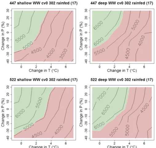
The median of the 30-year mean winter wheat yield ranged between ca. 3000 and ca. 7000 kg ha−1under perturbed P and T depending on soil and CO2level, as shown by the IRSs for standard management
(Fig. 3). The ensemble median yield was projected to increase with P and decrease with T, as expected. The shape of the yield isolines indi-cates that T became the limiting factor at high P increments (isolines tended to be vertical), while P became the limiting factor at low T incre-ments (isolines tended to be horizontal). Yield was lower for shallow than for deep soil, and increased with [CO2]. Depending on the soil
and CO2level, current yields were maintained up to 2–4 °C of T increase
at highest P increases. When P decreased up to 20%, baseline yields were maintained only at high [CO2] (522 ppm) together with small T
incre-ments of up to 2 °C (Fig. 3, green mask).
In general, for all the adaptations, the ARSs isolines did not change with elevated [CO2], but soil depth increased yield sensitivity to
precip-itation. Accordingly, the perturbations for which the current yield was recovered depended on soil depth and, to a lesser extent, [CO2].
Hereaf-ter, results for shallow soil and 447 ppm of CO2concentration are shown
(Figs. 4 to 8), as this would be the most unfavourable combination, while the other combinations are illustrated in suppl. Mat. (Figs. S2 to S22).
Thefirst single adaptation tested was removal of the vernalization requirements (Fig. 4e). An adaptation response between 10% and 40% was found depending on the T and P perturbation. This adaptation allowed current yield (green mask) to be recovered or exceeded for T perturbations up to +5 °C if P strongly increased, and for T perturba-tions up to +3 °C when P decreased up to−30%.
Other single adaptations were changes in cycle duration, sowing date and application of sI, all of them for winter wheat. Changing cycle duration or sowing date alone did not show any potential to overcome the negative impact (Figs. S2, S5, S11 and S17 in suppl. mat.). Applying sI atflowering resulted in an increased yield of potentially more than 30% (Fig. 5e). Current yield was recovered even for the greatest decreases of P and up to ca. 2 °C of T increase (green mask).
Table 2
Simulated yield (kg ha−1) for some combinations of adaptation options tested in the preliminary phase forΔP = −15%, ΔT = +2 °C and [CO
2] at 447 ppm. Simulated yields with no
adaptations and under baseline climate are reported as reference. Simulations were run with the CERES-wheat and SiriusQuality2 (SQ2) models, and adaptation options comprised: re-moving vernalization requirements (SWcv0), shortening crop cycle by 10% (WWcv1-10), lengthening crop cycle by 10% and 20% (WWcv2+10 and WWcv2+20, respectively), and sup-plementary irrigation (sI). These were combined with three sowing dates: 15 days before the standard sowing date (−15), 15 and 30 days after the standard sowing date (+15 and +30, respectively). The standard sowing date was set to day of the year 302. Results are shown for shallow and deep soils.
Sowing date No adaptation (360 ppm)
SWcv0 WWcv1-10 WWcv2+10 WWcv2+20 sI
CERES SQ2 CERES SQ2 CERES SQ2 CERES SQ2 CERES SQ2 CERES SQ2
Shallow soil 0 3825 2820 −15 3953 3482 3934 2103 3917 2256 3944 2301 3957 2761 +15 3244 2714 3152 2238 3267 2556 3241 2577 3318 3111 +30 2985 2943 2832 2388 3031 2590 2997 2591 3067 3062 Deep soil 0 6654 5640 −15 6927 6040 6608 5422 6375 5292 6164 5335 6875 5658 +15 6204 5715 5688 5585 5694 5620 5430 5557 6246 5856 +30 5837 5542 5202 5503 5508 5547 5201 5476 5940 5833
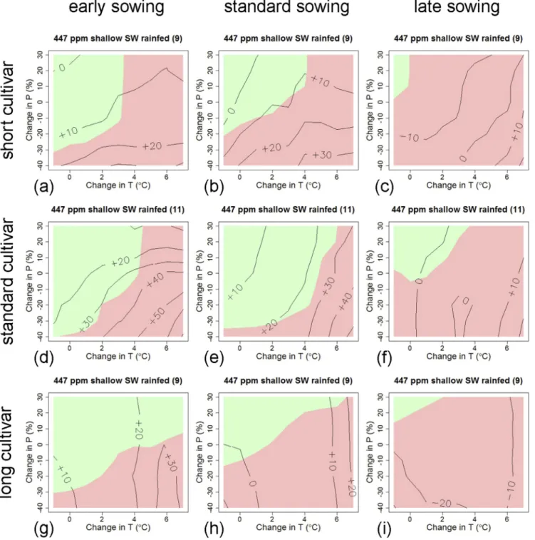
3.3.2. Combined adaptation options
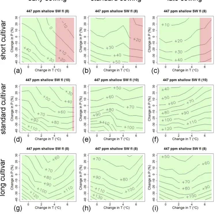
Thefirst set of combinations tested was based on rainfed SW, (i.e. with no vernalization requirements) (Fig. 4). The maximum adaptation response for rainfed SW was +60% (Fig. 4d). In general, the earlier the sowing date, the higher the adaptation response. The adaptation re-sponse to changes of cycle length was more variable. As an example, the shorter cultivar (SW-cv1) was more useful for compensating for the T effect, while the longer cultivar (SW-cv2) was more useful for dealing with the P effect, especially for the earlier sowing date (e.g.
Fig. 4a vs.Fig. 4g). When P decreased, only a few combined adaptation options allowed recovery of current yield and only for small increases in T: generally not higher than 2 °C. At higher T increases, maintaining current yield (recovery response) was only possible for the highest P increases.
Then, when sI atflowering was considered, maximum adaptation response for SW was + 80% (Fig. 6d). Also in this case, the earlier the sowing date the higher the adaptation response. The longer cultivar cycle (SW-cv2) provided a better adaptation response than the shorter one (SW-cv1). Although the standard cycle duration (SW-cv0) showed a strong adaptation response, only the longer cycle (SW-cv2) allowed recovery of current yields whatever the P and T perturbation (green mask,Fig. 6). The sI also revealed some adaptation potential for winter wheat (WW) (Fig. 5). Maximum adaptation response for the combina-tions based on sI and winter wheat was up to +30%. The standard cul-tivar (WW-cv0) showed an adaptation response whatever the sowing date, while the shorter cultivar (WW-cv1) only provided an adaptation response with earlier and standard sowing dates. For these cases, the higher the P decrease, the higher the adaptation response. Under these conditions the adaptation allowed maintenance of current yields
(recovery response) up to 3 °C of T increase. The longer cultivar (WW-cv2) did not present a useful adaptation response.
To explore the full potential of adaptations, and to provide a refer-ence for identifying yield ceilings, the adaptations were simulated under full irrigation (fI) (Fig. 7). Maximum adaptation response for the combinations based on fI and SW was + 130%. Both SW-cv0 and SW-cv2 obtained very high adaptation response whatever the sowing date. SW-cv1 was the only one unable to recover current yield when T increased more than ca. 4 °C. Generally, the adaptation effect was simi-lar whatever the T increase (isolines became almost horizontal) for the highest P decreases. Vertical shape of the green to red mask transition, indicates that simulated yield responses under full irrigation are to tem-perature alone (as expected).
3.3.3. Recommended adaptation options
Figs. 4 to 7have been shown to illustrate the response of the ensem-bles of crop models to different adaptation options (complete set of plots in Suppl. mat.). To identify the options with high adaptation po-tential (high increment on crop yield when the adaptation was applied), all possible combinations for both 447 ppm and 522 ppm of [CO2] for
both shallow and deep soils, were analysed. We focused our attention on perturbations including P decrease. Thus,five perturbation regions were defined: 1) ΔP from 0 up to −20% and ΔT up to +1.5 °C, 2) ΔP from 0 up to−20% and ΔT from 1.5 to +3 °C, 3) ΔP from −20% up to −40% and ΔT up to +1.5 °C, 4) ΔP from −20% up to −40% and ΔT from 1.5 to + 3 °C, and 5)ΔP from 0 up to −40% and ΔT higher than 3 °C. Recommendations refer to these perturbation regions, and they are summarized inTable 3.
Fig. 3. Impact response surfaces (IRSs) of yield (kg ha−1) for the standard cultivar (WW-cv0) under standard management, i.e. rainfed conditions and sowing date set to 302 (DOY). Results are shown for both shallow (left plots) and deep (right plots) soils, and for 447 ppm (upper plots) and 522 ppm (bottom plots) of [CO2]. The number of members in the ensemble is
indicated in brackets. Green (red) mask indicates absolute yield values greater (lower) than the reference yield (i.e. 30-year mean yield without adaptation under 360 ppm). (For interpretation of the references to colour in thisfigure legend, the reader is referred to the web version of this article.)
Rainfed WW-based combinations should be avoided in both soils as adaptation options produced recovery responses for only few of the per-turbations. Winter wheat is only recommended when combined with sI. Under this management, the standard cultivar is recommended with a wide range of sowing dates, while shorter cycle cultivars should be sown earlier. These options would show adaptation response up to se-vere P, T perturbations (for all T perturbations under P decline), while recovery response would be possible up to severe P perturbations and moderate T changes (regions 1 and 3). Longer cultivars should be avoided in both soils, even with sI.
Spring wheat was successful under a wide variety of conditions. Earlier sowing is recommended for both soils, and later sowing dates should be avoided. Standard sowing date can also be used when sI is applied, and with the standard cultivar under rainfed management. All cultivars can be used in the shallow soil, while the shorter cultivar is not recommended in the deep soil. Most of these options show adaptation response up to severe P, T perturba-tions (for all T perturbaperturba-tions under P decline), especially for the shal-low soil, while recovery response was mainly shown by standard and longer cultivars.
Fig. 4. Adaptation response surfaces (ARSs) of yield changes (%) from yields without adaptation (i.e. same soil and [CO2], but for the standard cultivar and management). All ARSs are for
spring wheat (SW)-based adaptation options under rainfed conditions in shallow soil and for 447 ppm of [CO2], combined with short (SW-cv1; a, b, c), standard (SW-cv0; d, e, f) and long
(SW-cv2; g, h, i) cultivars, and with early (287, DOY, a, d, g), standard (302, b, e, h) and late (332, c, f, i) sowing dates. Therefore, a total of 9 combined adaptations is shown. Number of members in the ensemble is in brackets. Green (red) mask indicates absolute yield values (kg ha−1) of the evaluated adaptation greater (lower) than the reference yield) (i.e. 30-year mean yield without adaptation, WW-cv0, sown at 302, rainfed, under 360 ppm). (For interpretation of the references to colour in thisfigure legend, the reader is referred to the web version of this article.)
The recommended options described above did not depend on [CO2].
3.3.4. Interannual and intermodel variability
This analysis was aimed at checking the interannual and intermodel variability values of the recommended options against former studies, so only the main trends are commented on here. To illustrate these checks, three of the recommended adaptation options are shown with colour masks representing the interannual CV and the IQR of model spread (Fig. 8). CV (no more than 40% in these examples) was in line with that shown in Pirttioja et al. (2015) for Lleida. Concerning intermodel variability, there is no clear pattern of the IQR of absolute yields with respect to changes in P and T. This could be related to the complexity of single model responses.
4. Discussion
In this paper we used, for thefirst time to our knowledge, an ensem-ble of crop models for investigating potential adaptation strategies for wheat. For that purpose, we introduced the AOCK and the ARS concepts for ensemble building and analysis respectively. Below, we discuss all these aspects in depth.
4.1. Calibration
The calibration process allowed the modellers to identify one of the possible set of crop model parameters values matching a limited set of field observations. This combination consists of several parameters that could compensate for approximations elsewhere (Wallach et al., 2014); therefore, we could have several combinations of parameters
matching observations, particularly when calibration data set is limited (equifinality). Due to general overparameterization of the crop simula-tion models (Wallach et al., 2014) and uncertainties related to experi-mental data, in some cases, relatively good calibration performance still did not guarantee reasonable response simulations. This could in our case be due to the limited set offield data used for calibration, main-ly based on yield,flowering and maturity dates from two years, which is a typical level of information available for crop model applications. However, adaptation is needed beyond locations where we have de-tailed, high quality data sets, and this study aims to deal with situation while new data can be generated or accessed. To overcome these limita-tions several recommendalimita-tions should be considered before model ap-plication: 1) more than one variable (and in-season variables if possible) should be taken into account in the calibration evaluation (Challinor et al., 2014; Kersebaum et al., 2015; Martre et al., 2015), 2)
an ensemble of models should be used, because doing so could compen-sate for individual models' deficiencies if the ensemble is not too small (Martre et al., 2015), and 3) the AOCK concept is also needed for checking vector quality and biological coherence. In this study we have adhered to all of these recommendations.
4.2. The adaptations
Our analysis demonstrated that“business-as-usual”, i.e. WW with standard cultivar and management, should be avoided in the future. The adaptations tested here constituted measures that can already be applied by farmers, as the main purpose of this study was to support and provide guidelines for implementing adaptation. Our preliminary phase and the existing literature allowed us to establish that a wide
range of phenology x sowing date combinations should be the starting point of any adaptation study in this Mediterranean environment.
Concerning single adaptation options, no single factor was able to overcome the detrimental effect of the complex interactions imposed by the P, T and [CO2] perturbations. The sole exception was sI, which
proved to be useful even under the most severe perturbations, probably due to the high dependency of Mediterranean rainfed cropping systems on precipitation (Oweis et al., 1998). This could be also true for current conditions. The analysed location, Lleida, is located in northeastern Spain and WW is currently grown; however, our results indicated that the latitudinal threshold of WW suitability would move towards higher latitudes under a warmer climate, in agreement withMínguez et al. (2007). The T increases affected WW vernalization, giving an advantage to SW. Concerning the less clear response of yield to changes in crop cycle duration, we hypothesized that the main cause was the
uncertainty related to the modelling of phenology. This uncertainty comes mainly from the different descriptions and simulations of crop phenology across crop models. For example, some models consider a simple accumulation of thermal time, while others take into account daylength and vernalization. Other models consider the number of leaves produced and the phyllochron or include the effect of water and nutrient stress. To test this hypothesis, we conducted a deeper anal-ysis of the implementation of the phenological options by the ensemble members,finding that the spread of the model response (the ensemble spread of the simulated phenological dates in days) partially masked the perturbations of the cycle duration imposed. This spread was com-parable to the number of days that corresponded to a 10% change of the crop cycle. We would need to simulate a larger phenological pertur-bation to overcome this effect. Such a simulation should be considered in future multi-model ensemble modelling exercises.
When combined adaptation options were considered, our results demonstrated that effective adaptation is possible at Lleida. Moreover, a wide scope of adaptation is opened up. Both WW and SW provided some adaptation response under certain combinations of cycle duration and sowing date. Early sowing emerged as a good option when com-bined with other options, confirming the findings byGiannakopoulos et al. (2009)andMoriondo et al. (2010), who tested the individual effect of this adaptation. This response could be influenced by the initial soil water content (in this exercise, set to 75% offield capacity). So prudence is needed when implementing this recommendation, as for lower initial soil water contents (e.g. for years with an extended dry period lasting into autumn, frequent under the weather conditions of southern Spain) a lower or even a worst response could be obtained by the earlier sowing.
In spite of the uncertainty on the implementation of phenology-based adaptations reported above, some conclusions about the duration of the growth cycle could nevertheless be extracted. Even when in prin-ciple adaptations based on longer-duration cultivars may appear advan-tageous with increasing temperatures (Giannakopoulos et al., 2009), our results showed that this might not always be the case for Lleida. This is probably because the expected yield gains due to the longer cycle would be offset by grainfilling happening in a warmer period. Ad-ditionally, extreme high temperatures could impose an absolute con-straint on wheat viability at the end of the cycle if longer-duration cultivars were to be considered as an adaptation option (Trnka et al., 2014; Pirttioja et al., 2015). Supplementary irrigation failed to overcome these effects for winter wheat. For SW, soil type made a difference for the adaptation potential of longer-duration cultivars, enabling the lon-ger-cycle crop to take advantage of the deep soil because of its higher water holding capacity.
Supplementary irrigation atflowering was found to present poten-tial for successful adaptation under many combinations of phenology
and sowing date. The use of sI at key phenological stages is in line with the current evolution already observed in the Mediterranean: e.g. in Andalusia the area under irrigation has been extended in recent de-cades, with no increase in total irrigation water used resulting from the promotion of deficit irrigation strategies (Lorite et al., 2012). Like-wise, in southern Italy irrigated areas are increasing as a result of the use of innovative irrigation systems (Acutis and Ventrella, 2015). Sup-plementary irrigation was not just useful for raising crop yields but in some cases also stabilized the effect of the adaptation when T increased (e.g.Fig. 6d), as previously also reportedOweis et al. (1998). When sI is applied, the choice of cycle duration can be used to stabilize adaptation effect against changing P (as cv2,Fig. 6g) or T (as cv1,Fig. 6a). It is im-portant to emphasize that several rainfed options showed adaptation potential for specific combinations of sowing date and phenology (see examples inTable 3). Full irrigation (fI) showed the greatest potential for supporting successful adaptation when water requirements were fulfilled, as all the T increases considered could be coped with by the fI option; this is in agreement with previous studies (Mínguez et al., 2007; Ruiz-Ramos et al., 2011).
In general, inter-annual variability was not affected by the adapta-tions, and median values of CV were consistent with those found for Lleida inPirttioja et al. (2015). This is because, by using the delta change approach for the sensitivity analysis combined with a seasonal pattern, we changed the intra-annual variability of climate but not the inter-an-nual variability. Therefore, the results may not necessarily hold true if the future interannual variability of the climatic variables are greatly dif-ferent from those employed. A separate study would be necessary to an-alyse this more comprehensively.
The effect of adaptation options on ensemble inter-model variability was evaluated by comparing the IQR for the adapted conditions to that for the unadapted baseline. Lleida cropping systems have been reported to be very sensitive to precipitation (Ruiz-Ramos and Mínguez, 2010),
Fig. 8. Adaptation response surfaces (ARSs) of yield change (%) for three adaptation options, comprising winter (WW) and spring (SW) wheat, shorter (cv1) and standard (cv0) cultivars, earlier (DOY = 287) and standard (DOY = 302) sowing dates, and rainfed and supplementary irrigation (sI) conditions for shallow soil and for 447 ppm of CO2. Number of members in the
ensemble is in brackets. Green to orange mask indicates: ensemble median of the 30-year interannual coefficient of variation (CV, %) (a, b, c); and ensemble interquartile range (IQR) (d, e, f) of absolute yields of the evaluated adaptation. IQR is expressed as percentage of the IQR for same soil, CO2level, standard cultivar and management for no T, P perturbations (IQRr), so
so it is not surprising that the uncertainty response from IQR analysis proved to be very complex. A separate study would be necessary to an-alyse this more comprehensively.
Finally, adaptation has to be tailored to local conditions (Reidsma et al., 2015). Our results demonstrated that, even for a single location, implementing an effective adaptation strategy depends on expected perturbation intensity and local environment (e.g. soil type), which is in agreement withIglesias et al. (2010). As a consequence of this, we cannot rely on just one single or combined adaptation option for a whole region or for all periods into the future in order to beflexible to changing conditions over time; moreover, the resultant recommenda-tions for adapting wheat might not be valid for other environments or periods. However, many of the results found here could still be valid for regions with decreased precipitation under climate change. 4.3. Ensemble building
Concerning ensemble building, some factors must be considered. First, we are aware that the ensemble size was different for several ad-aptations. Based on this, in drawing our conclusions we have avoided comparing options modelled from different ensembles; for such cases, the adaptations were evaluated separately. However, the number of members of the ensemble was always between 8 and 14, which matches the range of minimum ensemble sizes recommended in recent international crop model intercomparison exercises (e.g.Martre et al., 2015). Nevertheless, the robustness of an ensemble can be severely compromised if it includes model outcomes that are obviously implau-sible (see e.g.Rötter et al., 2012). Therefore (and secondly), for the de-cision on which models belong to the final ensemble, we have formalized here the concept of AOCK. This we have applied as an ex post plausibility check, using it to screen out crop responses judged to be unrealistic based on our current knowledge, rather than just
checking whether technical errors may have occurred. Similar criteria of plausibility were defined using IRSs for an ensemble of models of cli-mate change impact on permafrost byFronzek et al. (2011). We are per-fectly aware that empirical models should not be used outside the boundary conditions for which they were developed. Similarly, mecha-nistic models might provide unreliable outputs when applied in condi-tions that largely exceed the limits for which the model formalisms were developed; also, model calibrations are limited in their spatial and temporal coverage. A generalization of the AOCK concept or other equivalent procedures should be introduced for comprehensively interpreting model results in all kinds of modelling studies.
The AOCK concept is needed when our understanding of the pro-cesses involved is significantly lacking, or when high levels of uncertain-ty are inherent in a particular system analysis or simulation. In these situations, a combination of sound knowledge in comparable condi-tions, observed data and common sense can be used to check whether simulation results appear to be reasonable. For this particular study, the concept was applied through several criteria based on the following general principles: 1) plausible absolute values, 2) plausible ecophysio-logical responses to inputs (weather, soil and management), and 3) thresholds set sufficiently wide to include uncertainty in empirical data-bases, model parameters and structure, while excluding evidently im-plausible responses. These principles can be transferred to other modelling studies and for other crops and environmental conditions. It should be borne in mind that the AOCK concept always includes some degree of arbitrariness, in particular in the selection of the specific criteria to be met and the threshold values selected. The consequence of an excess of arbitrariness or inappropriate criteria definition (e.g. by set-ting too narrow thresholds) could be the exclusion of plausible but not very likely responses that could become more likely under unknown conditions (e.g. extreme divergent future conditions). To reduce this ar-bitrariness, the criteria used should be well-argued and transparently
Table 3
Perturbation regions for which specific options show positive adaptation and/or recovery responses, and derived recommendations. Perturbation regions are defined as follows (see em-bedded scheme in the table): region 1 is defined as ΔP from 0 up to −20% and ΔT up to +1.5 °C, region 2 is defined as ΔP from 0 up to −20% and ΔT from 1.5 to +3 °C, region 3 is defined as ΔP from −20% up to −40% and ΔT up to +1.5 °C, region 4 is defined as ΔP from −20% up to −40% and ΔT from 1.5 to +3 °C, and region 5 is defined as ΔP from 0 up to −40% and ΔT higher than 3 °C.
Shallow Deep
Water
mgnt Cultivar Sowing date Adaptation Recovery Adaptation Recovery Recommendations
WW R None None None None To be avoided
sI cv1 Earlier 1,2,3,4,5 1,2,3,4 1,2,3,4,5 1,2,3,4 Only under sI and
-Standard cultivar whatever the sowing date -Shorter cultivars own earlier
-Same recommendations for both soils
cv0 All 1,2,3,4,5 1 1,2,3,4,5 1,2,3
cv2 None None None To be avoided
SW R cv1 Earlier 1,2,3,4,5 1 3,4
Avoiding latest sowing
Advancing sowing whatever the cultivar Standard sowing with sI,and with standard cultivar under rainfed conditions
Shorter cultivar not recommended on deep soil
Standard 2,3,4,5 None 2,4,5 None
cv0 Standard & earlier 1,2,3,4,5 1,2 1,2,3,4,5 1
cv2 Earlier 1,2,3,4,5 1 1,2,3,4,5 1,2,3
sI cv1 Earlier 1,2,3,4,5 1,3 None
Standard 2,3,4,5 2,3 Not
recommended cv0 Standard & earlier 1,2,3,4,5 1,2,3,4 1,2,3,4,5 1,2,3,4 cv2 Standard & earlier 1,2,3,4,5 1,2,3,4,5 1,2,3,4,5 1,2,3,4,5
Abbreviations: rainfed (R), supplementary irrigation (sI), shorter, standard and longer crop cycle duration (cv1, cv0 and cv2 respectively), cultivar without vernalization requirements (SW), winter wheat (WW), management (mgnt), not considered because of lack of adaptation response (–).
– – – – – – –
documented to allow further refinement, and sensitivity of results to AOCK application and to the specific criteria definition should be analysed.
5. Conclusions
Three novelties were presented in this paper: 1) the use of an en-semble of crop models for supporting adaptation; 2) ARSs, which have proved to be a useful tool for planning adaptations under highly uncer-tain conditions; and 3) the formalization of the AOCK concept, which should be a driver for comprehensively interpreting model results in all modelling studies. Based on these, we conclude that effective tion at Lleida is possible. When locally addressed, the scope for adapta-tion widens and several soluadapta-tions might arise depending on the availability of irrigation. Thus, according to our results, there are few ad-aptation options that could work under rainfed conditions in Lleida. However, one single sI event was enough to create adaptation potential for many adaptation options based on simple changes of phenology and management. The study of recommendations for adaptation prioritized combined options based on SW, standard (current) and shorter cycle duration and early sowing date with sI. Many of these adaptations allowed maintenance of current yields for moderate T and P perturba-tions, some of them for severe perturbations as well.
Acknowledgements
This work wasfinancially supported by the Spanish National Insti-tute for Agricultural and Food Research and Technology (INIA, MACSUR01-UPM), the Italian Ministry of Agriculture and Forestry and the Finnish Ministry of Agriculture and Forestry (D.M. 24064/7303/15) through FACCE MACSUR− Modelling European Agriculture with Cli-mate Change for Food Security, a FACCE JPI knowledge hub; MULCLIVAR, from the Spanish Ministerio de Economía y Competitividad (MINECO, CGL2012-38923-C02-02); the Academy of Finland (deci-sions: 277276 and 277403), the EU FP7 IMPRESSIONS project (grant agreement no. 603416), the NORFASYS project (decision nos. 268277 and 292944) and PLUMES project (decision nos. 277403 and 292836); project IGA AF MENDELU no. 7/2015 with the support of the Specific University Research Grant provided by the Ministry of Education, Youth Sports of the Czech Republic; the Ministry of Education, Youth Sports of the Czech Republic within the National Sustainability Programme I (NPU I), grant number LO1415 NAZV QJ1310123 the Polish National Centre for Research and Development in frame of the projects: LCAgri, contract number BIOSTRATEG1/271322/3/NCBR/2015 and GyroScan, contract number BIOSTRATEG2/298782/11/NCBR/2016.
Appendix A. Supplementary data
Supplementary data to this article can be found online athttp://dx. doi.org/10.1016/j.agsy.2017.01.009.
References
Abeledo, L.G., Savin, R., Slafer, G.A., 2008.Wheat productivity in the Mediterranean Ebro Valley: analyzing the gap between attainable and potential yield with a simulation model. Eur. J. Agron. 28, 541–550.
Acutis, M., Ventrella, D., 2015.L'acqua, l'agricoltura e il clima che cambia. In: Mastrorilli, M. (Ed.), L'acqua in agricoltura. Gestione sostenibile della pratica irrigua, Edagricole, pp. 43–60.
Asseng, S., Ewert, F., Martre, P., Rötter, R.P., Lobell, D.B., Cammarano, D., Kimball, B.A., Ottman, M.J., Wall, G.W., White, J.W., Reynolds, M.P., Alderman, P.D., Prasad, P.V.V., Aggarwal, P.K., Anothai, J., Basso, B., Biernath, C., Challinor, A.J., De Sanctis, G., Doltra, J., Fereres, E., Garcia-Vile, M., Gayler, S., Hoogenboom, G., Hunt, L.A., Izaurralde, R.C., Jabloun, M., Jones, C.D., Kersebaum, K.C., Koehler, A.K., Muller, C., Kumar, S.N., Nendel, C., O'Leary, G., Olesen, J.E., Palosuo, T., Priesack, E., Rezaei, E.E., Ruane, A.C., Semenov, M.A., Shcherbak, I., Stockle, C., Stratonovitch, P., Streck, T., Supit, I., Tao, F., Thorburn, P.J., Waha, K., Wang, E., Wallach, D., Wolf, I., Zhao, Z., Zhu, Y., 2015.Rising temperatures reduce global wheat production. Nat. Clim. Chang. 5, 143–147.
Cartelle, J., Pedro, A., Savin, R., Slafer, G.A., 2006.Grain weight responses to post-anthesis spikelet-trimming in an old and a modern wheat under Mediterranean conditions. Eur. J. Agron. 25, 365–371.
Challinor, A.J., Watson, J., Lobell, D.B., Howden, S.M., Smith, D.R., Chhetri, N., 2014.A meta-analysis of crop yield under climate change and adaptation. Nat. Clim. Chang. 4, 287–291.
Collins, M., Knutti, R., Arblaster, J., Dufresne, J.-L., Fichefet, T., Friedlingstein, P., Gao, X., Gutowski, W.J., Johns, T., Krinner, G., Shongwe, M., Tebaldi, C., Weaver, A.J., Wehner, M., 2013.Long-term climate change: projections, commitments and irreversibility. In: Stocker, T.F., et al. (Eds.), Climate Change 2013: The Physical Science Basis. Contri-bution of Working Group I to the Fifth Assessment Report of the Intergovernmental Panel on Climate Change. Cambridge University Press, Cambridge and New York, pp. 1029–1136.
Diffenbaugh, N.S., Giorgi, F., 2012.Climate change hotspots in the CMIP5 global climate model ensemble. Clim. Chang. 114, 813–822.
Ferrise, R., Moriondo, M., Bindi, M., 2011.Probabilistic assessments of climate change im-pacts on durum wheat in the Mediterranean region. Nat. Hazards Earth Syst. Sci. 11, 1293–1302.
Fronzek, S., Carter, T.R., Raisanen, J., Ruokolainen, L., Luoto, M., 2010.Applying probabilis-tic projections of climate change with impact models: a case study for sub-arcprobabilis-tic palsa mires in Fennoscandia. Clim. Chang. 99, 515–534.
Fronzek, S., Carter, T.R., Luoto, M., 2011.Evaluating sources of uncertainty in modelling the impact of probabilistic climate change on sub-arctic palsa mires. Nat. Hazards Earth Syst. Sci. 11, 2981–2995.
Gabaldón-Leal, C., Lorite, I.J., Mínguez, M.I., Lizaso, J.I., Dosio, A., Sanchez, E., Ruiz-Ramos, M., 2015.Strategies for adapting maize to climate change and extreme temperatures in Andalusia, Spain. Clim. Res. 65, 159–173.
Giannakopoulos, C., Le Sager, P., Bindi, M., Moriondo, M., Kostopoulou, E., Goodess, C.M., 2009.Climatic changes and associated impacts in the Mediterranean resulting from a 2 °C global warming. Glob. Planet. Chang. 68, 209–224.
Grassini, P., Eskridge, K.M., Cassman, K.G., 2013. Distinguishing between yield advances and yield plateaus in historical crop production trends. Nat. Commun. 4:11.http:// dx.doi.org/10.1038/ncomms3918.
Harris, G.R., Collins, M., Sexton, D.M.H., Murphy, J.M., Booth, B.B.B., 2010.Probabilistic pro-jections for 21st century European climate. Nat. Hazards Earth Syst. Sci. 10, 2009–2020.
Hartmann, D.L., Klein Tank, A.M.G., Rusticucci, M., Alexander, L.V., Brönnimann, S., Charabi, Y.A.-R., Dentener, F.J., Dlugokencky, E.J., Easterling, D.R., Kaplan, A., Soden, B.J., Thorne, P.W., Wild, M., Zhai, P., 2013.Observations: atmosphere and surface. In: Stocker, T.F., et al. (Eds.), Climate Change 2013: The Physical Science Basis. Contri-bution of Working Group I to the Fifth Assessment Report of the Intergovernmental Panel on Climate Change. Cambridge University Press, Cambridge and New York, pp. 159–254.
Iglesias, A., Quiroga, S., Schlickenrieder, J., 2010.Climate change and agricultural adapta-tion: assessing management uncertainty for four crop types in Spain. Clim. Res. 44, 83–94.
IPCC, 2013. Annex I: Atlas of Global and Regional Climate Projections Supplementary Ma-terial RCP8.5 [van Oldenborgh, G.J., Collins, M., Arblaster, J., Christensen, J.H., Marotzke, J., Power, S.B., Rummukainen, M., Zhou, T. (eds.)]. In: Stocker, T.F., et al. (Eds.), Climate Change 2013: The Physical Science Basis. Contribution of Working Group I to the Fifth Assessment Report of the Intergovernmental Panel on Climate Change Available from.www.climatechange2013.org.www.ipcc.ch.
Jamieson, P.D., Porter, J.R., Wilson, D.R., 1991.A test of the computer-simulation model ARCHWHEAT1 on wheat crops grown in New-Zealand. Field Crop Res. 27, 337–350.
Jones, J.W., Hoogenboom, G., Porter, C.H., Boote, K.J., Batchelor, W.D., Hunt, L.A., Wilkens, P.W., Singh, U., Gijsman, A.J., Ritchie, J.T., 2003.The DSSAT cropping system model. Eur. J. Agron. 18, 235–265.
Kersebaum, K.C., Boote, K.J., Jorgenson, J.S., Nendel, C., Bindi, M., Fruhauf, C., Gaiser, T., Hoogenboom, G., Kollas, C., Olesen, J.E., Rötter, R.P., Ruget, F., Thorburn, P.J., Trnka, M., Wegehenkel, M., 2015.Analysis and classification of data sets for calibration and validation of agro-ecosystem models. Environ. Model. Softw. 72, 402–417.
Lorite, I.J., Garcia-Vila, M., Carmona, M.A., Santos, C., Soriano, M.A., 2012.Assessment of the irrigation advisory services' recommendations and farmers' irrigation manage-ment: a case study in southern Spain. Water Resour. Manag. 26, 2397–2419.
Martre, P., Jamieson, P.D., Semenov, M.A., Zyskowski, R.F., Porter, J.R., Triboi, E., 2006.
Modelling protein content and composition in relation to crop nitrogen dynamics for wheat. Eur. J. Agron. 25, 138–154.
Martre, P., Wallach, D., Asseng, S., Ewert, F., Jones, J.W., Rötter, R.P., Boote, K.J., Ruane, A.C., Thorburn, P.J., Cammarano, D., Hatfield, J.L., Rosenzweig, C., Aggarwal, P.K., Angulo, C., Basso, B., Bertuzzi, P., Biernath, C., Brisson, N., Challinor, A.J., Doltra, J., Gayler, S., Goldberg, R., Grant, R.F., Heng, L., Hooker, J., Hunt, L.A., Ingwersen, J., Izaurralde, R.C., Kersebaum, K.C., Muller, C., Kumar, S.N., Nendel, C., O'Leary, G., Olesen, J.E., Osborne, T.M., Palosuo, T., Priesack, E., Ripoche, D., Semenov, M.A., Shcherbak, I., Steduto, P., Stockle, C.O., Stratonovitch, P., Streck, T., Supit, I., Tao, F.L., Travasso, M., Waha, K., White, J.W., Wolf, J., 2015.Multimodel ensembles of wheat growth: many models are better than one. Glob. Chang. Biol. 21, 911–925.
Metzger, M.J., Bunce, R.G.H., Jongman, R.H.G., Mücher, C.A., Watkins, J.W., 2005.A climatic stratification of the environment of Europe. Glob. Ecol. Biogeogr. 14, 549–563.
Mínguez, M.I., Ruiz-Ramos, M., Diaz-Ambrona, C.H., Quemada, M., Sau, F., 2007. First-order impacts on winter and summer crops assessed with various high-resolution cli-mate models in the Iberian Peninsula. Clim. Chang. 81, 343–355.
Montesino-San Martin, M., Olesen, J.E., Porter, J.R., 2015.Can crop-climate models be ac-curate and precise? A case study for wheat production in Denmark. Agric. For. Meteorol. 202, 51–60.
Moriondo, M., Bindi, M., Kundzewicz, Z.W., Szwed, M., Chorynski, A., Matczak, P., Radziejewski, M., McEvoy, D., Wreford, A., 2010.Impact and adaptation opportunities