HAL Id: hal-00296990
https://hal.archives-ouvertes.fr/hal-00296990
Submitted on 26 Apr 2007
HAL is a multi-disciplinary open access
archive for the deposit and dissemination of
sci-entific research documents, whether they are
pub-lished or not. The documents may come from
teaching and research institutions in France or
abroad, or from public or private research centers.
L’archive ouverte pluridisciplinaire HAL, est
destinée au dépôt et à la diffusion de documents
scientifiques de niveau recherche, publiés ou non,
émanant des établissements d’enseignement et de
recherche français ou étrangers, des laboratoires
publics ou privés.
On evaluation of ensemble precipitation forecasts with
observation-based ensembles
B. Ahrens, S. Jaun
To cite this version:
B. Ahrens, S. Jaun. On evaluation of ensemble precipitation forecasts with observation-based
ensem-bles. Advances in Geosciences, European Geosciences Union, 2007, 10, pp.139-144. �hal-00296990�
www.adv-geosci.net/10/139/2007/ © Author(s) 2007. This work is licensed under a Creative Commons License.
Geosciences
On evaluation of ensemble precipitation forecasts with
observation-based ensembles
B. Ahrens1and S. Jaun2
1Institute for Atmosphere and Environment, University of Frankfurt, Germany 2Institute for Atmospheric and Climate Science, ETH Zurich, Switzerland
Received: 4 August 2006 – Revised: 5 January 2007 – Accepted: 19 January 2007 – Published: 26 April 2007
Abstract. Spatial interpolation of precipitation data is
un-certain. How important is this uncertainty and how can it be considered in evaluation of high-resolution probabilistic precipitation forecasts? These questions are discussed by ex-perimental evaluation of the COSMO consortium’s limited-area ensemble prediction system COSMO-LEPS. The ap-plied performance measure is the often used Brier skill score (BSS). The observational references in the evaluation are (a) analyzed rain gauge data by ordinary Kriging and (b) ensem-bles of interpolated rain gauge data by stochastic simulation. This permits the consideration of either a deterministic ref-erence (the event is observed or not with 100% certainty) or a probabilistic reference that makes allowance for un-certainties in spatial averaging. The evaluation experiments show that the evaluation uncertainties are substantial even for the large area (41 300 km2) of Switzerland with a mean rain gauge distance as good as 7 km: the one- to three-day pre-cipitation forecasts have skill decreasing with forecast lead time but the one- and two-day forecast performances differ not significantly.
1 Introduction
Weather forecast systems have to be evaluated. Nowadays, limited-area numerical weather prediction models provide meteorological forecasts with kilometer-scale horizontal grid spacing. High-resolution precipitation forecasts are of pri-mary interest. For example, in flood forecasting systems the precipitation details are a crucial input parameter.
A typical distance between precipitation observation sites with daily observation frequency in the European Alps is 10 km (cf. Fig. 1 for the distribution of precipitation stations in Switzerland). This is a comparatively dense observation
Correspondence to: B. Ahrens ([email protected])
network but precipitation is a quantity with high spatial vari-ability. Therefore, it is a valid question to ask if such a den-sity of observations allows for evaluation of daily precipita-tion forecasts in mountainous catchments with a typical area as small as about 1500 km2?
Recently, ensemble prediction systems (EPS) became op-erational which predict forecast probabilities by integration of an ensemble of numerical weather prediction models from slightly different initial states and model parameters (Ehren-dorfer, 1997; Palmer, 2000). The motivation for the EPS is that the spread in the ensemble forecasts indicates forecast uncertainty and the interpretation of the forecast probabili-ties provides better results than interpretation of one single deterministic forecast that is initiated by the best known but nethertheless uncertain atmospheric state. Zhu et al. (2002) showed with a simple cost-loss model that for most users the ensemble forecasts offer a higher economic value than the deterministic forecast.
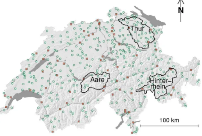
Here, EPS precipitation forecasts of the limited-area EPS COSMO-LEPS (Montani et al., 2003) with grid-spacing of 10 km are evaluated for the year 2005 for Switzerland and for three selected catchments (cf. Fig. 1). These three catch-ments are one pre-alpine catchment, the Thur, and two alpine catchments, the Aare (part of an elongated wet anomaly ex-tending along the northern rim of the Alps) and the Hinter-rhein (relatively dry inner-alpine area).
For the evaluation exercise presented here, we apply the commonly used Brier skill score (BSS). The BSS assess the probability forecasts of dichotomous events (e.g. the proba-bility of more than 10 mm precipitation in the period and area of interest). In BSS application the observational reference is typically assumed to be certain: the observed event prob-ability is either zero or one. The uncertainty in the observed catchment precipitation is often neglected.
This and the advantage of generating ensembles of inter-polated observational fields, i.e. a probabilistic reference, through stochastic simulations is discussed in Sect. 4. Before
140 B. Ahrens and S. Jaun: On evaluation of ensemble precipitation forecasts
Fig. 1. Switzerland (total area: 41 300 km2) and three catch-ments named Thur (1700 km2), Aare (1200 km2), and Hinterrhein (1500 km2). The circles show the locations of the rain station net-work ALL and the subset indicated by the red crosses show the locations of the network SUB.
that we introduce the available observational data and the evaluated limited-area EPS. Finally, evaluation results with and without observation uncertainty will be discussed in Sect. 5 and some concluding remarks will be given.
2 Precipitation data
This paper investigates precipitation in Switzerland and smaller catchments in the year 2005. The considered tem-poral resolution of the evaluation is daily. The reference are precipitation data as observed by the Swiss conventional precipitation station network available through the national weather service MeteoSwiss with about 430 stations in 2005 and a mean next-neighbor distance of about 7 km. The data from this dense network is named ALL here. Also con-sidered in the evaluation is a coarser data subset observed by 65 stations, which are located close to stations of the au-tomatic measurement network ANETZ of MeteoSwiss with mean next-neighbor station distance of about 17 km. This subset resembles the data availability in case of near real-time evaluation or in less densely observed regions and is named SUB. ANETZ data itself is not applied to avoid prob-lems with mixing of different station types in the evaluation. The spatial distributions of the two station sets are illus-trated in Fig. 1. Within the considered catchments the num-bers of stations are of the order of ten in case of ALL but only of two in case of SUB. Therefore, differences in evalu-ation with the different data sets are to be expected.
3 Limited-area prediction system COSMO-LEPS
The experimentally evaluated ensemble data are forecast by the consortium for small-scale modeling limited-area
ensem-ble prediction system COSMO-LEPS (Montani et al., 2003, and http://www.cosmo-model.org). The COSMO-LEPS im-plementation is formally validated in Marsigli et al. (2005). We selected the year 2005 as our evaluation period, since it has been without major changes in the operational LEPS set-up. In that period the ensemble size was set to ten and each ensemble member’s forecast with grid-spacing of 10 km was initiated each day at 12:00 UTC. Here precipitation simula-tions for the forecast hours 18 to 42 h, 42 to 66 h, and 66 to 90 h (the one-, two-, and three-day forecasts, respectively) are assessed.
Each LEPS member is nested into a different representa-tive forecast of a coarser-grid global EPS (the operational ensemble forecast of the European Centre of Medium Range Forecasts, Reading). These representative global members are selected by grouping the global members into ten clus-ters based on the analysis of wind and vorticity fields over a domain covering most of Europe (Molteni et al., 2001). From each cluster the central member (with minimum distance to all cluster members) is chosen to host a limited-area forecast. In the evaluation presented below we consider limited-area EPS members either weighted with cluster size or not.
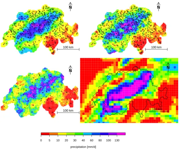
Figure 2 shows the one-day forecast of the LEPS member that is driven by the most representative member (the cen-tral member from the cluster with about 25% of the global members) for 21 August 2005. This precipitation event led to major flooding in the northern European Alps. Also given in Fig. 2 are interpolated precipitation observations (cf. next section). The forecast depicts the coarse-scale features of the precipitation pattern but also over-estimates precipitation substantially in the central region of the event.
4 Evaluation method
The direct model output at grid-box scale should not be ap-plied and some temporal and spatial smoothing of the output is recommended for being numerically representative (e.g. Grasso, 2000; Ahrens, 2003). Here, daily catchment means of precipitation are evaluated with averages over at least 15 model grid-boxes and thus the forecasts can be assumed rep-resentative. But how to estimate representative observational references from the limited number of rain gauge stations available? This has to be done by interpolation and averag-ing to the catchment scale.
Here, we apply ordinary Kriging with a spherical ogram model as one interpolation method. Kriging vari-ants are often proposed and applied in precipitation analysis (Creutin and Obled, 1982; Atkinson and Lloyd, 1998; Beck and Ahrens, 2004). For the necessary variogram estimation we adopted a sub-optimal but robust approach (Ahrens and Beck, 2006). From the daily data of the year 2005 we esti-mated from standardized observations a climatological vari-ogram range to about 40 km with a sill of 1 (mm/d)2(by con-struction). For daily analyses the sill is rescaled with the data
N 100 km N 100 km N 100 km N 100 km 0 5 10 20 30 40 60 80 100 130 precipitation [mm/d]
Fig. 2. Precipitation of 21 August 2005 in Switzerland as interpolated by Kriging (upper left panel), by stochastic simulation with ALL
stations (upper right) or SUB stations (lower left), and as predicted by a 1-day forecast of the most representative COSMO-LEPS member (lower right). The locations of the considered stations are indicated by small circles.
variance. For either data set, ALL and SUB, a local neigh-borhood of 8 stations is considered in interpolation. Figure 2 shows the Kriging analysis for the day 21 August 2005 with ALL data.
Kriging is an example of a data-fitting technique. There-fore, it is expected that the interpolated fields underestimate the true field variance (the smoothing relationship of Kriging states that the interpolated field variance at any location is the data variance minus the Kriging variance) with the con-sequence that the variance of the catchment time series is underestimated. More important in evaluation is that the es-timation of the interpolation errors is extremely difficult in case of precipitation since the stationarity and normality as-sumptions of Kriging are not very well fulfilled. Here, the areal precipitation estimate through ordinary Kriging is con-sidered a deterministic observational reference (DOR) be-cause no uncertainty in interpolation is considered.
An alternative interpolation approach is based on stochas-tic simulation of an ensemble of precipitation fields with conditioning on the available station data. The idea is to simulate stochastically field realizations that “honor” the ob-served data, their point values, their areal mean, and their
covariance structure (Journel, 1974; Chil`es, 1999; Ahrens and Beck, 2006). Therefore, the spatial variability is rep-resented more realistically in the stochastic realizations than in Kriging. For the evaluation exercise a large ensemble of observation-based realizations is generated and thus a prob-abilistic observational reference (POR) is available. This al-lows the comparison of probabilistic EPS forecasts against the POR by comparison of probability distributions. Addi-tionally, an ensemble of comparisons against the multiple realizations reference (MRR) of the observational ensemble can be performed and the spread in these comparisons pro-vides a precision measure for the evaluation without trou-blesome estimation and interpretation of the Kriging vari-ance. Averaging the ensemble of observation-based realiza-tions yields a data-fitting technique (and this mean interpo-lator is thus smoother than any ensemble member) and is in the limit of large ensembles equivalent to a Kriging approach. The ensemble average yields another DOR in the following evaluation.
Stochastic interpolation is done by conditioned sequen-tial Gaussian simulation (e.g., Johnson, 1987; Chil`es, 1999, Chap. 7) as it is implemented in the geostatistical software
142 B. Ahrens and S. Jaun: On evaluation of ensemble precipitation forecasts 0 10 20 30 40 0 10 20 30 40 Precip(Obs) [mm/d] Precip(LEPS) [mm/d]
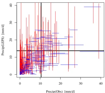
Fig. 3. The median LEPS 1-day forecasts versus the median observation-based stochastic interpolations of the SUB network. The precipitation values are daily and Swiss averages. The bars in-dicate the 90% confidence intervals of the forecasts (red) and of the interpolations (blue). The thick black lines give the 90th percentiles of the interpolations (10.5 mm/d) and the forecasts (13.8 mm/d).
package “gstat” (Pebesma, 2004). Sequential simulation in-volves the generation of a Gaussian random field, condi-tioned to the observed data, that honors the variogram of the random field. Since daily precipitation is a non-Gaussian, non-negative process, the data has been normalized by a log-arithmic transformation and applying variogram estimates for the transformed data based on rescaling of the climato-logical variogram with an estimated climatoclimato-logical range of about 100 km. For each day and data set an ensemble of realizations with one hundred members is generated and ap-plied in the following comparisons. Each ensemble member is less accurate than the Kriging analysis in a squared-error sense by construction, but respects the covariance structure given by the observations.
Figure 2 shows two realizations of stochastic interpolation: one is conditioned on ALL and the other on SUB obser-vations. As expected the stochastic interpolation is rougher than Kriging. Additionally, it can be seen that the condition-ing by ALL is more restrictive than by SUB by comparison with the Kriging interpolation of the dense ALL network data. Figure 3 illustrates that in case of the SUB network there is even for daily and Swiss averages substantial scatter in the observational reference. The scatter is even larger for the smaller catchments (not shown).
Optimal interpolation of precipitation fields is an active field of research. The remaining deficiencies of the Krig-ing analysis and stochastic simulation upscalKrig-ing motivate the discussion of the advantages of PORs over DORs.
Neverthe-less, the applied methods are state-of-the-art for daily high-resolution precipitation interpolation.
An often applied performance measure in evaluation of probabilistic forecasts also applied here is the Brier skill score, BSS, (cf. Stanski et al., 1989; Wilks, 2006, and references wherein). The BSS compares probability fore-casts Yt=P (yt≤y0)at dates t =1, 2, . . ., T of forecast events
yt≤y0(y0is a chosen event threshold: e.g. 10 mm/d in case of precipitation forecasts yt) with the observed event prob-abilities Ot=P (xt≤x0) of some observational quantity xt with related threshold x0. Commonly, the observations are assumed perfect and thus Ot ∈ {0, 1} – the event occurred or did not. This is the assumption made in evaluation with DOR. Figure 3 shows that our knowledge about observed event occurrence is uncertain: for several precipitation days the 90th percentile threshold is within the confidence inter-val of the reference inter-values. Therefore, POR has to be applied and the Ot’s codomain is the interval [0, 1].
The BSS is defined by
BSS = 1 − BS(Y, O)
BS(C, O) (1)
with the Brier score
BS(Y, O) = 1/T T
X
t =1
(Yt− Ot)2 (2)
The BS is essentially the mean squared error of the proba-bilistic forecast. The BS(C, O) of some climatological fore-cast C is introduced as a reference forefore-cast in the BSS for normalization. The skill score equals one in case of perfect forecasts (a perfect forecast of an uncertain observational ref-erence is uncertain itself) and zero if the evaluated forecast skill compares to the skill of the climatology.
The estimation of forecast probabilities from small EPS leads to biased BSS values (M¨uller et al., 2005). The COSMO-LEPS ensemble size is ten only. Therefore, we de-biased the BSS following Weigel et al. (2006). The clima-tological probability of some precipitation forecast thresh-old can not be estimated reliably because of the short pe-riod of available COSMO-LEPS data. We applied instead the 90th percentiles in 2005 depending on the data-set (forecast or observation-based, catchment) as thresholds. For exam-ple, the threshold for the kriged reference with ALL data in Switzerland is 9.5 mm/d, for the stochastically interpo-lated realizations 9.7 mm/d, and for the EPS forecasts about 13.5 mm/d. This data-set dependent selection of thresholds is equivalent to some forecast post-processing and improves the BSS.
5 Results
As mentioned above the probabilistic EPS forecasts are usu-ally compared against deterministic references (DORs). This
Table 1. BSS values for the 1-,2-, and 3-day COSMO-LEPS forecasts with weighted members. Different observational refer-ences based on ALL observations are applied in the BSS estima-tion: (a) deterministic observational references (DOR) by Krig-ing/averaging of ensembles of stochastically interpolated fields, (b) multiple stochastic realizations (MRR) yielding an BSS ensemble (the first and third quartiles of the BSS distributions are given), and (c) probabilistic references (POR).
1 day 2 days 3 days Switzerland DOR .44/.45 .42/.45 .36/.33 MRR .44–.48 .43–.45 .31–.33 POR .48 .46 .34 Thur DOR .44/.46 .36/.37 .27/.28 MRR .39–.44 .32–.37 .24–.28 POR .45 .37 .28 Hinterrhein DOR .20/.18 .18/.17 .19/.17 MRR .18–.20 .17–.18 .17–.20 POR .20 .18 .19 Aare DOR .37/.36 .29/.20 .25/.21 MRR .31–.36 .18–.22 .21–.24 POR .38 .23 .26
paper generates DORs either by Kriging or by averaging en-sembles of stochastic interpolations of the precipitation ob-servations followed by averaging to the evaluation areas. For large ensembles applying the same variogram models etc. these references converge. Here, the observational ensemble consists of one hundred members and there are differences in the climatological variogram and data normalization. Table 1 shows that these differences yield differences in the BSS. It is interesting to note that the second method gives slightly better BSS in the larger and relatively better observed areas (Switzerland and Thur) and slightly worse results in the more difficult areas (Hinterrhein and Aare with relatively less ob-servations, but also, as the smaller BSS values indicate, the more challenging forecast regions).
Table 1 also shows the inter-quartile range of BSS val-ues if the probabilistic forecasts are compared against the stochastic MRRs. The spread is substantial and larger than the differences between the deterministic results. For exam-ple, taking the spread into account the performance of one- or two-day forecasts for Switzerland do not differ significantly (the inter-quartile ranges overlap) for the 10% heaviest rain events which are evaluated in this paper. The forecasts for the Hinterrhein are less good as for the other areas and there is no significant difference between one-, two-, and even three-day forecasts. In this area only rather large-scale rain events are well forecasted and those are well represented in the EPS quite independent of the forecast lead time (not shown).
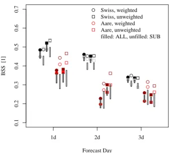
Forecast Day BSS [1] 0.1 0.2 0.3 0.4 0.5 0.6 0.7 1d 2d 3d Swiss, weighted Swiss, unweighted Aare, weighted Aare, unweighted filled: ALL, unfilled: SUB
Fig. 4. BSSs of ensemble forecasts in the Swiss and Aare areas.
The darker symbols (black, dark red) indicate evaluation against the probabilistic reference, the lighter symbols (grey, light red) indicate evaluation against the deterministic ensemble mean reference, the bars indicate the inter-quartile range of evaluation results against single members of the observational ensemble, and the filled and unfilled symbols and bars show the results for the networks ALL and SUB, respectively. Bullets and squares with the close-by bars discriminate between weighted and unweighted forecast ensembles, respectively.
Also given in the Table are the BSSs if the probabilistic forecasts are evaluated against PORs. These BSSs tend to be better than for the deterministic or single member evalu-ations. This is not surprising since in this case Ot can take values between zero and one and – remembering that the BS is a quadratic difference – this leads to smaller BSs and larger BSSs as long as the observational uncertainty is smaller than the forecast uncertainty. This is a welcome feature since an uncertainty in the observational reference should not punish the forecasts.
Figure 4 clearly shows that the evaluation uncertainty is larger for the smaller Aare catchment than for Switzerland. At the same time the forecast performance is at least one day better in the larger area. Again the consideration of the refer-ence uncertainty through the PORs increases the BSSs. The difference in probabilistic or deterministic reference evalua-tion is especially large, as expected, in the Aare catchment if the coarse observation network SUB is considered.
As mentioned in Sect. 3 the LEPS members can be weighted by the size of the global forecast clusters. This should lead to better forecasts in general but not necessarily for Switzerland since the clustering is based on large-scale weather patterns. Figure 4 indicates that the one-day fore-cast for Switzerland is insignificantly better with unweighted members and that for two- and three-day forecast weighting marginally improves the forecasts. In case of the smaller
144 B. Ahrens and S. Jaun: On evaluation of ensemble precipitation forecasts
Aare area the weighting is detrimental for one- and two-day forecasts. Non-uniform weighting decreases the spread in the forecast ensembles (the inter-quartile ranges in the forecast ensemble are 2.8 mm/d for the weighted and 2.9 mm/d for the unweighted one-day forecasts in the year-long average) and thus yields more extreme Yts and smaller BSS values. For longer lead times the evaluation areas are increasingly in-fluenced by large-scale weather patterns leading to the global clusters and thus the optimal selection of the global represen-tative members yields an increase in spread (4.6 mm/d with and 4.5 mm/d without for three-day forecasts) and this favors weighting (although insignificantly because of the evaluation uncertainty).
6 Conclusions
It is common practice in evaluation of probabilistic areal precipitation forecasts that the observational reference is as-sumed perfect neglecting spatial interpolation errors. This paper shows that generating ensembles of stochastically in-terpolated fields conditioned on the available data is a simple method for consideration of interpolation uncertainty in the evaluation. These ensembles allow the determination of en-sembles of comparisons if the forecast is compared against every single ensemble member. The spread in the compari-son ensemble easily delivers an evaluation uncertainty. This is demonstrated by estimation of ensembles of Brier skill score (BSS) values in evaluation. Additionally, the obser-vational ensembles can be considered as a probabilistic ref-erence in a probabilistic evaluation. This yields higher BSS values than with single, deterministic reference evaluation, and this is fair since in doubt it should be assumed that the forecasts perform well. Therefore, we suggest application of a reference ensemble for (a) estimation of evaluation uncer-tainty and (b) the estimation of the potentially best perfor-mance of the forecast given the reference’s uncertainty.
Additional sources of evaluation uncertainty have to be considered besides horizontal interpolation errors. In moun-tainous areas the vertically inhomogeneous distribution of stations can lead to systematic errors. Further, wind and evaporation loss of the rain gauges yields precipitation under-catch up to several ten percent. These error sources addition-ally illustrate how challenging the evaluation of precipitation forecasts in small areas is and will be with ever increasing resolution of forecasts and forecast applications.
Acknowledgements. Data are provided by MeteoSwiss, Zurich. S.
J. acknowledges support through NCCR-Climate, funded by the Swiss National Science Foundation.
Edited by: S. C. Michaelides and E. Amitai Reviewed by: anonymous referees
References
Ahrens, B.: Evaluation of precipitation forecasting with the limited area model ALADIN in an Alpine watershed, Meteorol. Z., 12,
245–255, 2003.
Ahrens, B. and Beck, A.: On upscaling of rain–gauge data for eval-uating numerical weather forecasts, Meteorol. Atmos. Phys., in print, 2007.
Atkinson, P. and Lloyd, C.: Mapping precipitation in Switzerland with ordinary and indicator Kriging, J. Geographic Information and Dec. Analysis, 2, 65–76, 1998.
Beck, A. and Ahrens, B.: Multiresolution evaluation of precipita-tion forecasts over the European Alps, Meteorol. Z., 13, 55–62, 2004.
Chil`es, J.-P.: Geostatistics: modeling spatial uncertainty, John Wi-ley & Sons, New York, 1999.
Creutin, J. and Obled, C.: Objective analyses and mapping tech-niques for rainfall fields: an objective comparison, Water Resour. Res., 18, 413–431, 1982.
Ehrendorfer, M.: Predicting the uncertainty of numerical weather forecasts: a review, Meteorol. Z., 6, 147–183, 1997.
Grasso, L. D.: The differentiation between grid spacing and reso-lution and their application to numerical modeling, Bull. Amer. Meteorol. Soc., 81, 579–580, 2000.
Johnson, M.: Multivariate Statistical Simulation, Wiley, New York, 1987.
Journel, A.: Geostatistics for conditional simulation of ore bodies, Econom. Geol., 69, 673–687, 1974.
Marsigli, C., Boccanera, F., Montani, A., and Paccagnella, T.: The COSMO-LEPS mesoscale ensemble system: validation of the methodology and verification, Nonlin. Processes Geophys., 12, 527–536, 2005,
http://www.nonlin-processes-geophys.net/12/527/2005/. Molteni, F., Buizza, R., Marsigli, C., Montani, A., Nerozzi, F., and
Paccagnella, T.: A strategy for high-resolution ensemble predic-tion. I: Definition of representative members and global-model experiments, Quart. J. Roy. Meteorol. Soc., 127, 2069–2094, 2001.
Montani, A., Capaldo, M., Cesari, D., Marsigli, C., Modigliani, U., Nerozzi, F., Paccagnella, T., Patruno, P., and Tibaldi, S.: Opera-tional limited-area ensemble forecasts based on the Lokal Mod-ell, ECMWF Newsletter, 98, 2–7, 2003.
M¨uller, W., Appenzeller, C., Doblas-Reyes, F., and Liniger, M.: A debiased ranked probability skill score to evaluate probabilistic ensemble forecasts with small ensemble sizes, J. Climate, 18, 1513–1523, 2005.
Palmer, T. N.: Predicting uncertainty forecasts of weather and cli-mate, Rep. Prog. Phys., 63, 71–116, 2000.
Pebesma, E.: Multivariable geostatistics in S: the gstat package, Comp. & Geosci., 30, 683–691, 2004.
Stanski, H., Wilson, L., and Burrows, W.: Survey of common veri-fication methods in meteorology, Tech. Rep. WMO/TD No. 358, WMO World Weather Watch, 1989.
Weigel, A., Liniger, M., and Appenzeller, C.: The discrete Brier and ranked probability skill scores, Mon. Wea. Rev., 135, 118–124, 2007.
Wilks, D. S.: Statistical Methods in the Atmospheric Sciences, Aca-demic Press, San Diego, 2006.
Zhu, Y., Toth, Z., Wobus, R., Richardson, D., and Mylne, K.: The economic value of ensemble–based weather forecasts, Bull. Amer. Meteorol. Soc., 83, 73–83, 2002.