Araar : Département d’économique and CIRPÉE, Pavillon DeSève, Université Laval, Québec, Canada G1K 7P4
Duclos : Département d’économique and CIRPÉE, Pavillon DeSève, Université Laval, Québec, Canada G1K 7P4
We are grateful to the PEP programme of IDRC, to Canada’s SSHRC, and to Québec’s FQRSC for financial Cahier de recherche/Working Paper 07-35
Poverty and Inequality Components: a Micro Framework
Abdelkrim Araar Jean-Yves Duclos
Abstract:
This paper explores the link between poverty and inequality through an analysis of the poverty impact of changes in income-component inequality and in between -and within- group inequality. This can help shed light on the theoretical and empirical linkages between poverty, growth and inequality. It might also help design policies to improve both equity and welfare. The tools are illustrated using the recent 2004 Nigerian national household survey. The analytically derived linkages are supported by the empirical illustration, and interesting insights also emerge from the empirical analysis. One such insight is that both the sign and the size of the elasticities can be quite sensitive to the choice of measurement assumptions (such as the choice of inequality and poverty aversion parameters, and that of the poverty line). The elasticities are also very much distribution-sensitive and dependent on the type of inequality-changing processes taking place. This also suggests that the response of poverty to growth can also be expected to be significantly context specific.
Keywords: Poverty, inequality, poverty elasticities, redistribution JEL Classification: D63, I32, O12
1 Introduction
The recent years have witnessed an increasingly strong interest in the im-pact of development on poverty. An important reason for this has been the establishment of the so-called Millennium Development Goals, which have set poverty reduction as a fundamental objective of development. The most fre-quently advocated manner to achieve such poverty reduction is through economic growth. Whether growth reduces poverty, and whether in particular growth can be deemed to be “pro-poor”, depends, however, on the impact of growth on in-equality and on how much this impact on inin-equality feeds into poverty. This link between growth and inequality has also generated considerable independent in-terest lately — see, among many relatively recent contributions to that debate,
Bruno, Ravallion, and Squire (1998), United Nations (2000), World Bank 2000,
Eastwood and Lipton (2001),Dollar and Kraay (2002), andBourguignon (2003).
This interest is of course reminiscent of the sempiternal debate on the ex-istence of a Kuznets (1956) inverted U-shape relationship between growth and inequality. It has more recently been mixed with the issue of how glob-alization affects poverty and inequality — see inter alia World Bank (2002),
Watkins (2002) and Heshmati (2004). Some recent empirical studies, such as
Deininger and Squire (1998) and Frazer (2006), have tended to conclude that
there exists little support for the Kuznets hypothesis, suggesting, as we ex-plore in this paper, that the relationship may be more complex and more het-erogeneous than is sometimes thought. This is also supported by the view of
Dollar and Kraay (2002) that although, on average, growth may have a neutral
impact on inequality, this impact exhibits considerable variability across time and space.
A closely related issue is whether we should be normatively interested in the impact of growth on absolute poverty or on relative inequality. This issue is at the heart of the debate surrounding the conceptual definition of “pro-poorness” — see, for instance, McCulloch and Baulch (1999), Kakwani and Pernia (2000),
Ravallion and Datt (2002), Kakwani, Khandker, and Son (2003),
Ravallion and Chen (2003),Klasen (2003),Son (2004) andEssama-Nssah (2005)
for recent contributions to that conceptual definition. The debate essentially involves the confrontation of different value judgments, and as such there does not seem to be a generally acceptable solution to it other than saying that both poverty and inequality can be of concern to analysts. Because of this, the link between poverty and inequality should also be of interest from a policy perspective. Are there changes in inequality that would be particularly effective at
reducing poverty? Are there policies that would be good at reducing both poverty and inequality? A major objective of this paper is to provide tools to help answer such questions.
The link between growth, inequality and poverty is also particularly impor-tant from a dynamic perspective. The recent World Development Report of the
World Bank (2005) encapsulated one aspect of this link in the phrase
“inequal-ity traps”, by which it is meant that inequal“inequal-ity may be self-reinforcing, hindering growth, and hampering poverty reduction in the longer term:
“The existence of these inequality traps — with mutually reinforcing inequalities in economic, political, social, and cultural domains — has two main implications for this analysis. The first implication is that, because of market failures and of the ways in which institutions evolve, inequality traps can affect not only the distribution but also the aggregate dynamics of growth and development. This in turn means that, in the long run, equity and efficiency may be complements, not substitutes.” (World Bank 2005, p.22)
This suggests that it may be appropriate to look at the combined effect of policy on — and at the joint evolution of — poverty and relative inequality even if we are normatively interested only in long-term absolute poverty alleviation.
We may finally be interested in the link between inequality and poverty for purely descriptive or accounting purposes. For instance, how do changing dispar-ities between regions or socio-demographic groups help explain the evolution of poverty? How are changes in inequality within these groups impacting poverty? How can poverty changes be linked to changes in the distribution of factor in-comes — such as changes in the composition of wage earners and self-employed workers, for instance, or changes in factor prices — both between and within socio-economic categories? Concerns are indeed often voiced that widening dis-parities across space (e.g., involving coastal vs inner regions, or urban vs rural areas) or increasing inequality between and within groups (e.g., skilled vs un-skilled workers, formal vs informal workers) may be pushing up poverty, or at least dampening the impact of growth on poverty. Again, the paper provides tools to help examine such issues.
The overall aim of this paper is thus to develop an analytical micro framework with which to probe into some of the complex and context-specific linkages that exist between poverty and inequality. One of the paper’s important results is to bring out the importance of making precise what type of inequality we have in
mind when we attempt to link poverty, inequality and growth. Another outcome is to help simulate the potential impact of economic shocks and economic policies on both poverty and inequality.
To achieve this, the paper derives a variety of elasticities of poverty and inequality with respect to various types of distributive changes. This is con-ceptually analogous to, but methodologically different from, the assessment of the contribution of growth and changes in inequality to the evolution of poverty in Datt and Ravallion (1992), Kakwani (1997), Shorrocks (1999) and
Araar and Awoyemi (2006), for instance; the paper’s analytical developments also
extend those ofKakwani (1993).
The rest of the paper is as follows. Section 2 presents an analytical deriva-tion of the poverty and inequality impact of different sources of distributive changes, all of them leading to increases in some types of inequality. We con-sider two main sources of such changes: changes in the inequality of socio-economic groups, and changes in the inequality of income components — see also
Essama-Nssah and Lambert (2006) andSon (2006) for recent — though
method-ologically different — attempts to track the impact of changes in income compo-nents on the pro-poorness of growth. For each of these sources of variations in inequality, we consider both “within” and “between” changes in inequality. We also consider changes in income-component inequality that affect only those in-dividuals that are effectively active in some economic sector — as opposed to changes that affect everyone’s income from that sector. This provides a rich set of contexts in which to analyze the relationship between poverty and inequality. Section 3then applies the analytical methods to a recent survey of incomes in a large developing country, Nigeria, in which both poverty alleviation and inequal-ity reduction form important elements of the strategy towards the achievement of the Millennium Development Goals. Section4summarizes the main results of the paper.
2 Poverty and inequality elasticities
2.1 Notation
Let incomes be non-negative and distributed according to the distribution func-tion F (y), assumed for exposifunc-tional simplicity to be continuous and with density function f (y). A quantile function Q(p) is then defined implicitly as F (Q(p)) ≡
income below which we find a proportion p of the population; it is also the in-come at percentile p in the population. Let µ be overall average inin-come, namely,
µ = R Q(p)dp. The Lorenz curve L(p), which gives the proportion of total
in-come that accrues to the poorest p proportion of the population, is then defined as
L(p) = µ−1
Z p
0
Q(q)dq, (1)
and the (ordinary) Gini index is given by:
I = 2
Z 1
0
(p − L(p))dp. (2)
Equation (2) uses the well-known definition of the Gini as twice the area be-tween the line of perfect equality, p, and the actual Lorenz curve, L(p). One can, however, also think of percentile-dependent weights to aggregate the distances
p − L(p). A popular one-parameter functional specification for such weights is
given by κ(p; ρ) = ρ(ρ − 1)(1 − p)ρ−2and depends on the value of a single
nor-mative parameter ρ. That parameter must be greater than 1 for the weights to be positive everywhere. We then obtain the class of Single-Parameter Gini (or S-Gini) indices as1
I(ρ) =
Z 1
0
(p − L(p))κ(p; ρ)dp. (3)
Yaari (1988) defines “an indicator for the policy maker’s degree of equality
mind-edness at p” as (ρ − 1)(1 − p)−1. The larger the value of ρ, the greater the
’mind-edness’ for equality, the relatively larger the value of κ(p; ρ) for small p, and therefore the greater the relative weight attributed to the distances between p and
L(p) at lower values of p. Let ω(p; ρ) then be defined as ω(p; ρ) =
Z 1
p
κ(q; ρ)dq = ρ(1 − p)ρ−1. (4)
Integration by parts of (3) leads to
I(ρ) = µ−1
Z 1
0
(µ − Q(p))ω(p; ρ)dp, (5)
1These were introduced by Donaldson and Weymark (1980), Kakwani (1980),
Donaldson and Weymark (1983), and Yitzhaki (1983); see also Duclos and Araar (2006), Section 4.2, for a discussion of the some of the properties of these indices.
and a special case of (5) is the ordinary Gini index of (2): I(2) = 2 µ Z 1 0 (µ − Q(p))(1 − p)dp. (6)
Let (1 − Q(p)/z)+ = max(0, (1 − Q(p)/z)) be the normalized poverty gap at
p. TheFoster, Greer, and Thorbecke (1984) (FGT) class of poverty indices is then
defined as P (z; α) = Z 1 0 µ z − Q(p) z ¶α + dp (7)
for a poverty line z and a “poverty-aversion” parameter α. It is well known that the popular poverty headcount and average poverty gap indices are given respectively by α = 0 and α = 1. The best-known inequality and poverty indices are thus particular members of the S-Gini and FGT classes of indices in (5) and (7). This explains why we focus on these classes in this paper. Note that both of these classes are normatively flexible since they incorporate an inequality and a poverty aversion parameter that can be varied by analysts. One outcome of the paper is indeed to see how the link between poverty and inequality is sensitive to such aversion parameters.
2.2 Changes in inequality
Changing the S-Gini index by 1%, say, can be done in a very large number of ways, each of them involving different transformations of the original income distribution. It can be seen for instance from (5) that changes in I(ρ) can come from distributive changes at the top of the income scale (large Q(p)), at the bottom (low Q(p)), or from changes involving both low and large incomes. This also means that a 1% change in inequality can be expected to generate many different impacts on poverty, depending on the precise nature of the distributive change that leads to it. In general, therefore, it does not seem appropriate to think of poverty and inequality as being linked deterministically across time or space. This is in fact one of the main (and, for micro-data analysts, somewhat obvious) lessons explored in this paper: a given change in inequality is compatible with many different possible changes in poverty. In fact, even if we restrict considerably and parameterize the type of distributive changes allowed to generate this 1% change in inequality — as we do below — the link between poverty and inequality still remains very heterogeneous and will depend inter alia on the precise nature of the change in inequality that is being considered.
A general type of distributive change that can be handled nicely from an an-alytical perspective spreads all incomes away from the mean by a proportional factor λ. It corresponds, roughly speaking, to an increased bipolarization of in-comes away from an unchanged mean — see for instance Wolfson (1994) and
Duclos and ´Echevin (2005). Such bipolarization is equivalent to adding (λ −
1)(Q(p) − µ) to each Q(p), in such a way that the post-bipolarization p-quantile equals:
Q(p; λ) = Q(p) + (λ − 1) (Q(p) − µ)
| {z }
increased bipolarization
. (8)
Note that this bipolarization does not affect average income since: Z 1 0 Q(p; λ)dp = Z 1 0 [Q(p) + (λ − 1) (Q(p) − µ)] dp = µ. (9)
The post bipolarization Lorenz curve is moved by a factor proportional to the distance between the line of perfect equality, p, and the initial Lorenz curve:
L(p; λ) = L(p) − (λ − 1) (p − L(p))
| {z }
increased bipolarization
. (10)
The post-bipolarization S-Gini index is then given by
I(ρ; λ) = µ−1
Z 1
0
λ(µ − Q(p))ω(p; ρ)dp, (11)
and it thus follows that
∂I(ρ; λ) ∂λ ¯ ¯ ¯ ¯ λ=1 = I(ρ; λ). (12)
At λ = 1, the bipolarization derivative of the S-Gini index is thus simply the S-Gini index itself.
2.3 Changes in poverty
The impact of bipolarization on FGT poverty is not as straightforward as in (12). To see why, first define P (z; α; λ) as poverty after the change in bipolariza-tion: P (z; α; λ) = Z 1 0 µ z − Q(p; λ) z ¶α + dp. (13)
The poverty impact of a change in λ can then be shown to be given by: ∂P (z; α; λ) ∂λ ¯ ¯ ¯ ¯ λ=1 = α£P (z; α) +¡µ−zz ¢P (z; α − 1)¤ if α > 0 f (z)(µ − z) if α = 0. (14)
Kakwani (1993) first derived this result; see also Duclos and Araar (2006) and
Appendix 1 of this paper for an alternative demonstration. The sign of (14)
de-pends on whether z exceeds µ or not. There are three cases:
1. For µ > z, (14) is unambiguously positive whatever the value of α.
2. For µ = z, (14) is zero for α = 0 and positive otherwise.
3. For µ < z, (14) is clearly negative for α = 0. For greater values of α, note that (14) can be rewritten as:
αz−α Z 1 0 [(µ − z) + (z − Q(p))](z − Q(p))α−1+ dp (15) = αz−α Z 1 0 (µ − Q(p))(z − Q(p))α−1 + dp (16) = αz−αcov¡µ − Q(p), (z − Q(p))α−1+ ¢ (17) ½ > 0 if α ≥ 1 > − < 0 if α < 1. (18)
In a very poor society, for which µ < z, decreasing the S-Gini will move some of those above µ into poverty and will thus increase the poverty headcount. As (18) indicates, an increase in inequality can also increase P (z; α) whenever α < 1.
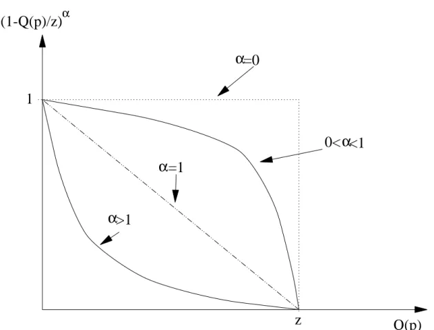
To see better why this is so, consider Figure1. The contribution of different quantiles Q(p) to total poverty is shown for different values of α. That contribu-tion is nil for quantiles Q(p) exceeding z. It is always non increasing with Q(p). Depending on the value of α, the contribution can be convex (when α ≥ 1) or sometimes concave in Q(p) (for lower values of α). Because of this, and depend-ing on the value of the incomes that are spread further from each other, poverty can either increase or decrease.
When increased bipolarization is applied to incomes in an area over which the contributions in Figure 1 are convex, poverty increases2; otherwise, poverty can
decrease. For instance, with α < 1, the curve in Figure1has two areas, one over which increased bipolarization reduces poverty — when increased bipolarization involves only the poor, and especially so if the richer of the poor then cross the poverty line — and another area over which increased bipolarization increases poverty (whenever increased bipolarization transfers involves a poor and a non-poor).3
Hence, even in the very simple case just considered, the impact on poverty of a change in inequality depends on initial conditions — namely, on the initial distribution of income and on whether z exceeds mean income — and on the way in which poverty is measured. The elasticity of FGT poverty with respect to the S-Gini is then obtained as
ελ(z; α; ρ) = ∂P (z; α; λ)/∂λ ∂I(ρ; λ)/∂λ I(ρ; λ) P (z; α; λ) ¯ ¯ ¯ ¯ λ=1 , (19)
which, using (12) and (14), leads to
ελ(z; α; ρ) = ( α h 1 +¡µ−zz ¢P (z;α−1)P (z;α) i if α > 0, f (z) F (z)(µ − z) if α = 0. (20)
As for (14), the sign of (20) depends on the values of z and α and on the distri-bution of incomes. The numerical value of (20) now also depends on the initial value of P (z; α), another source of variability across distributions. Note also that this particular type of elasticity does not explicitly depend on the initial value of
I(ρ).
2.4 Poverty and inequality within and between groups
To consider the impact of changes in within-group inequality, let g = 1, ..., G denote G exclusive and exhaustive socio-demographic groups (differentiated by regions of residence or by family characteristics, for instance) and let φ(p; g) be the proportion of those individuals at percentile p that belong to group g. This proportion is naturally bounded between 0 and 1. For example, if there were only two groups in a discrete population, noted by A and B, and 5 individuals located at some percentile p, two of them belonging to group A and the three others to
3Note that the sign of (16) depends on the sign ofRF (z)
0 [(µ − Q(p))]ς(p)dp, where ς(p) =
(z − Q(p))α−1. When α = 1, we have that ς(p) = 1 ∀p and (16) is greater than zero since
µ > F (z)−1RF (z)
group B, then we would have φ(p; A) = 0.40 and φ(p; B) = 0.60. The overall share of group g in the population is φ(g) = R φ(p; g)dp. The mean income of
group g is then denoted as
µ(g) = φ(g)−1
Z 1
0
Q(p)φ(p; g)dp (21)
and the overall mean is obtained as
µ = G X g=1 Z 1 0 Q(p)φ(p; g)dp. (22) 2.4.1 Within-group inequality
Within-group-g bipolarization spreads Q(p) away from µ(g) for those who belong to group g. This can be, for instance, caused by changes in the dispersion of physical and humain assets within a group as well as by changes in the returns to these assets. To see the effect of this, let σ(g) be a group-g-specific factor of bipolarization and let Q(p; g; σ(g)) be the expected post-bipolarization income of those in group g that were initially at percentile p in the overall distribution of income. Then,
Q(p; g; σ(g)) = Q(p) + (σ(g) − 1) (Q(p) − µ(g)) . (23)
Note that this scheme does not affect between-group inequality since average in-come µ(g) remains the same for all groups, whatever the value of σ(g):
φ(g)−1
Z
[Q(p) + (σ(g) − 1) (Q(p) − µ(g))] φ(p; g)dp = µ(g). (24)
The expected income of those initially at p is given by
Q(p; φ(g))) = Q(p) (1 − φ(p; g)) + Q(p; g; φ(g))φ(p; g). (25)
Now denote as I(ρ; σ(g)) the overall S-Gini after the bipolarisation factor σ(g) has been applied to the within-group-g distribution of income:
I(ρ; σ(g)) =
µ−1
Z
The impact on total inequality of a marginal increase in within-group-g inequality is then obtained as ∂I(ρ; σ(g)) ∂σ(g) ¯ ¯ ¯ ¯ σ(g)=1 = µ−1 Z 1 0 (µ(g) − Q(p)) ω(p; ρ)φ(p; g)dp (27) = φ(g)µ(g) µ IC (ρ; g) (28) where IC (ρ; g) = (φ(g)µ(g))−1 Z 1 0 (µ(g) − Q(p)) ω(p; ρ)φ(p; g)dp (29)
is the “coefficient of concentration”4of group g obtained by setting to µ(g), in (5),
the incomes of all those who do not belong to group g, and by normalizing (29) by φ(g)µ(g) — which is the contribution of group g to overall mean income.
Now denote by P (z; α; g) the FGT index for group g, formally defined as
P (z; α; g) = φ(g)−1 Z 1 0 µ z − Q(p) z ¶α + φ(p; g)dp. (30)
P (z; α; g; σ(g)) is obtained from (30) by replacing Q(p) by Q(p; σ(g)). Total
FGT poverty being given by
P (z; α; σ(g)) = X
g
φ(g)P (z; α; g; σ(g)), (31)
we therefore have that
∂P (z; α; σ(g))
∂σ(g) = φ(g)
∂P (z; α; g; σ(g))
∂σ(g) . (32)
Letting f (g; z) be the density of group g at z, we find:
∂P (z; α; σ(g)) ∂σ(g) ¯ ¯ ¯ ¯ σ(g)=1 = (33) αφ(g) h P (z; α; g) + ³ µ(g)−z z ´ P (z; α − 1; g) i if α > 0, φ(g)f (z; g)(µ(g) − z) if α = 0. (34) 4See for example Sections 7.2 and 7.3 of Duclos and Araar (2006) for an introduction to
Using (28) and (34), the elasticity of total poverty with respect to within-group inequality is then given by
εσ(g)(z; α; ρ) = ∂P (z; α; σ(g))/∂σ(g) ∂I(ρ; σ(g))/∂σ(g) I(ρ; σ(g)) P (z; α; σ(g)) ¯ ¯ ¯ ¯ σ(g)=1 . (35)
Note that the same comments as for (14) and (19) apply to the interpretation of the value of (35) — namely, that the sign and the magnitude of εσ(g)(z; α; ρ) depend
on α, z − µ(g) and the distribution of income in group g. Denoting by σ the case in which the same σ(g) is applied simultaneously to all groups, we then have
εσ(z; α; ρ) = ∂P (z; α; σ)/∂σ ∂I(ρ; σ)/∂σ I(ρ; σ) P (z; α; σ) ¯ ¯ ¯ ¯ σ=1 . (36) 2.4.2 Between-group inequality
We now consider the impact of a bipolarization process that spreads groups apart from each other without affecting within-group inequality. This change could come, for instance, from widening disparities across space — such as those between coastal and inner regions, urban and rural areas — or across groups — such as disparities between skilled and unskilled workers, or formal and infor-mal workers. To model this, we keep constant both within-group inequality and overall mean income by setting a between-group bipolarization factor γ(g) as a function of a scalar γ (common to all γ(g)):
γ(g) − 1 = 1 + (γ − 1) µ 1 − µ µ(g) ¶ . (37)
Expected post-bipolarization income for those initially at p and in group g is then given by Q(p; g; γ) = Q(p)(γ(g) − 1) (38) = Q(p) µ 1 + (γ − 1) µ 1 − µ µ(g) ¶¶ . (39)
Note that such between-group bipolarisation does not affect within-group inequal-ity since (38) amounts to multiplying all incomes in a group g by the same scalar
(γ(g) − 1). We also find for all values of γ that G X g=1 Z Q(p; g; γ)φ(p; g)dp = G X g=1 φ(g)µ(g) · 1 + (γ − 1)(µ(g) − µ) µ(g) ¸ (40) = " µ + (γ − 1) G X g=1 φ(g) (µ(g) − µ) # = µ, (41)
which confirms that such between-group polarization keeps overall mean income constant. Note that with this γ scheme, the average income of group g can be written as µ(g; γ) = µ(g) µ 1 + (γ − 1) µ 1 − µ µ(g) ¶¶ = µ(g) + (γ − 1) (µ(g) − µ) . (42)
Equation (42) shows that the impact of γ on average group income is similar to the impact of bipolarisation on incomes presented in equation (8). Clearly, increasing
γ thus increases between-group inequality. I(ρ; γ) is then given by
I(ρ; γ) = µ−1 G X g=1 Z 1 0 [µ − Q(p; g; γ)] φ(p; g)ω(p; ρ)dp (43)
The impact of a change in γ on the S-Gini can then be derived as5: ∂I(ρ; γ) ∂γ ¯ ¯ ¯ ¯ γ=1 = IC (ρ) + G X g=1 φ(g) µ µ(g) µ − 1 ¶ IC (ρ; g), (44)
where IC (ρ; g) is as in (29) and IC (ρ) is the coefficient of concentration obtained when everyone is assigned his group income:
IC (ρ) = µ−1 G X g=1 Z 1 0 (µ − µ(g)) ω(p; ρ)φ(p; g)dp. (45)
IC (ρ) is thus an index of between-group inequality.
Note that if all individuals within a given group are identical, (44) reduces to (12). If within-group inequality is not zero, however, then we must also take
into account its role (through IC (ρ; g)). (45) implicitly assumes that all incomes within a group are changed by the same absolute value, which is equivalent to assuming no within-group inequality. Increasing between-group bipolarization has instead the effect of increasing everyone’s income by the same proportion
γ(g)−1. In the presence of within-group inequality, higher incomes in a group are
therefore affected absolutely more, and lower incomes less, than what is captured by (45). For µ(g) < µ, this has the effect of decreasing inequality, and the reverse for µ(g) > µ. The net effect of this is captured byPGg=1φ(g)
³
µ(g) µ − 1
´
IC (ρ; g).
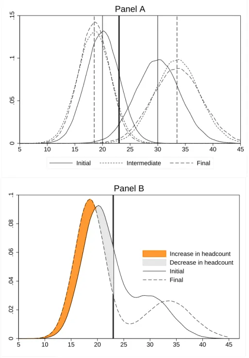
Figure2contains an illustrative example of how between-group bi-polarization affects inequality and poverty. The continuous lines in Panel A show the initial density functions within each of two subgroups. These densities are moved to the short-dashed lines with the increase in between-group inequality6. Since these
movements change within-group inequality, a second adjustment is required to keep within-group inequality unchanged; this is shown by the movement from the short-dashed to the long-dashed lines of Panel A. For the group to the left of Panel A, this movement to a long-dashed line decreases inequality; the converse is true for the group to the right of Panel A. As shown in Panel B of Figure2, and as noted analytically above in (44), these movements have opposite effects on inequality.
The poverty impact of such between-group bipolarisation equals7:
∂P (z; α; γ) ∂γ = (46) αPGg=1φ(g) ³ µ µ(g) − 1 ´ [zP (z; α − 1; g) − P (z; α; g)] if α > 0 PG g=1φ(g) ³ µ µ(g) − 1 ´ f (z; g) if α = 0. (47)
The elasticity of total poverty with respect to between-group bipolarization is then denoted by εγ(z; α; ρ) and is defined by
εγ(z; α; ρ) = ∂P (z; α; γ)/∂γ ∂I(ρ; γ)/∂γ I(ρ; γ) P (z; α; γ) ¯ ¯ ¯ ¯ γ=1 . (48)
The poverty impact of between-group bipolarization is thus qualitatively am-biguous, depending in particular on the relation of average group incomes µ(g) to
6The same constant amount c is added (or subtracted) for each group; as shown by
Araar (2006), this has the effect of changing the Gini by −c
µI.
overall average income, and on within-group poverty P (z; α; g). This can again be seen in Panel B of Figure2, where between-group bipolarization and the move-ment from the continuous to the dashed line generate two conflicting effects on the headcount.
2.5 Poverty and inequality in income components
Now consider the joint impact on inequality and poverty of changes in the inequality of income components (or income sources). To do this, first suppose that the sum of a total number K of income components equals total income and that the expected amount of income component k found at percentile p is denoted by s(p; k). We have that Q(p) = K X k=1 s(p; k). (49)
The overall mean of income component k is then given by µ(k) = R s(p; k)dp.
Note that s(p; k) can be increasing or decreasing with p (and can even be negative if component k is a tax or a capital income loss for instance).
2.5.1 Within-component inequality
Increasing the bipolarization of income component k amounts to increasing the distance between overall mean component and the individual value of all in-come components. This is also obtained by adding (η(k) − 1)(µ(k) − s(p; k)) to
s(p; k) in such a way that expected income at percentile p becomes
Q(p; η(k)) = Q(p) + (η(k) − 1) (s(p; k) − µ(k)) . (50)
Examples of the sources of such a change are increased dispersions in the inequal-ity of the distribution of human (education, experience, abilinequal-ity) or of physical capital. We then have:
I(ρ; η(k)) = µ−1
Z
[µ − (Q(p) + (η(k) − 1)(s(p; k) − µ(k)))] ω(p; ρ)dp. (51)
The impact on inequality of a change in η(k) is then
∂I(ρ; η(k)) ∂η(k) ¯ ¯ ¯ ¯ η(k)=1 = ψ(k)IC (ρ; k), (52)
where ψ(k) = µ(k)/µ is the share of income component k in total income and
IC (ρ; k) is the usual coefficient of concentration of component k:
IC (ρ; k) = µ(k)−1 Z (s(p; k) − µ(k))ω(p; ρ)dp. (53) Letting P (z; α; η(k)) = Z 1 0 µ z − Q(p; η(k)) z ¶α + dp, (54)
the impact on total poverty of within-component increased bipolarization is then8 ∂P (z; α; η(k))
∂η(k) =
½
αz−1µ(k)£P (z; α − 1) − CD(z; α; k)¤ if α > 0
−f (z)(s(F (z); k) − µ(k)) if α = 0, (55)
where CD(z; α; k) isMakdissi and Wodon (2002)’s normalized consumption-dominance curve for component k:
CD(z; α; k) = Z 1 0 µ z − Q(p) z ¶α−1 + s(p; k) µ(k) dp. (56)
Note that CD(z; α; k) is an average of the percentile share, s(p; k)/µ(k), of com-ponent k times poverty gaps to the power α − 1. As for (14), (55) can be positive or negative, depending on z, α, µ(k), and the distribution of s(p; k). In particular, the sign of the impact on the poverty headcount (α = 0) depends on the differ-ence between the expected level of income component k at the poverty line and the overall mean value of that component. If s(F (z); k) exceeds µ(k), the head-count will fall following an increase in the inequality of component k. That would occur, for instance, if an increase in the bipolarization of farm income applied to a distribution in which some of the not-so-poor poor had greater farm income than average farm income — a situation that is plausible.
The elasticity of total poverty with respect to within-component inequality is then denoted as εη(k)(z; α; ρ) and is defined as
εη(k)(z; α; ρ) = ∂P (z; α; η(k))/∂η(k) ∂I(ρ; η(k))/∂η(k) I(ρ; η(k)) P (z; α; η(k)) ¯ ¯ ¯ ¯ η(k)=1 (57) 8See Appendix 4 for a demonstration.
Note that a scheme η obtained by applying the same η(k) to all income compo-nents is equivalent to the scheme λ in (8) since
Q(p; η) = Q(p) + (η − 1) K X k=1 (s(p; k) − µ(k)) (58) = Q(p) + (η − 1) (Q(p) − µ) . (59)
We then have that
εη(z; α; ρ) ≡ ελ(z; α; ρ). (60)
2.5.2 Between-component inequality
Increased between-component inequality is generated by an increase in the bipolarisation of average income components without changing within-component inequality. Changes in relative consumption and factor prices can produce this naturally. To model this process while keeping overall mean constant, we define a component-specific factor τ (k) of change in the average of component k,
τ (k) − 1 = 1 + (τ − 1) µ 1 − µ/K µ(k) ¶ , (61)
and we obtain the expected value of post-bipolarization component k at percentile
p as s(p; k) µ 1 + (τ − 1) µ 1 − µ/K µ(k) ¶¶ . (62)
Multiplying s(p; k) by a factor that is independent of p maintains constant within-component-k inequality. The expected incomes of those initially at percentile p then become Q(p; τ ) = Q(p) + K X k=1 s(p; k) µ (τ − 1) µ 1 − µ/K µ(k) ¶¶ . (63)
Using the common factor τ also maintains constant the value of overall mean income since by (63) we have
Z 1 0 Q(p; τ )dp = µ + K X k=1 (τ − 1) µ 1 −µ/K µ(k) ¶ Z 1 0 s(p; k)dp (64) = µ + (τ − 1) K X k=1 ³ µ(k) − µ K ´ = µ. (65)
With this scheme, the mean of income component k becomes µ(k; τ ) = µ(k) µ 1 + (τ − 1) µ 1 −µ/K µ(k) ¶¶ = µ(k) + (τ − 1) (µ(k) − µ/K) , (66)
which implies an increase in between-component analogous to (8). The marginal impact on the S-Gini of a change in τ is then given by9:
∂I(ρ; τ ) ∂τ ¯ ¯ ¯ ¯ τ =1 = " I − K X k=1 IC (ρ; k) K # , (67)
whereas the poverty impact of this increased bipolarisation equals10: ∂P (z; α; τ ) ∂τ ¯ ¯ ¯ ¯ τ =1 = α h P (z; α) − P (z; α − 1) + µz PKk=1 CD(z;α;k)K i if α > 0 −f (z)PKk=1s(F (z); k)³1 −µ/Kµ(k)´ if α = 0. (68)
The elasticity of total poverty with respect to between-component inequality is then denoted as ετ(z; α; ρ) and defined simply by replacing γ by τ in (48).
2.6 Within- and between-component inequality revisited
Section 2.5 models the poverty and inequality impact of increasing the dis-tance between each value of income component k and overall mean component
µ(k) at each percentile p. This is the traditional approach to this sort of inequality
decompositions. Increasing within- or between-group inequality affects all of the values of a group’s incomes; similarly, increasing within- or between-component inequality affects all of the values of an income component.
It is sometimes useful, however, to see how variations in an income component
k affects only the group with, say, a positive level of the component. It may indeed
be easier to implement policies that reduce income-source inequality only among those who are already active in an economic sector. An alternative approach to Section2.5would therefore be to increase the inequality in component k for only a portion of the population, such as those with a positive value for component k (e.g., those with a positive level of formal labor market earnings), or those that also belong to some socio-demographic group (such as to consider the non-farm income of rural households, for instance), or those whose total income falls below some threshold (such as those below some poverty line).
9See Appendix 5 for a demonstration. 10See Appendix 6 for a demonstration.
2.6.1 Truncated within-component inequality
For expositional simplicity, suppose therefore that we are interested in the impact of increasing the earnings bipolarization of those actively engaged in the labor market (and thus with a positive value of such earnings). Let ϕ(p; k) be the proportion of individuals at percentile p that have a positive level of earnings, and let ϕ(k) = R ϕ(p; k)dp be the overall population share of those with positive
earn-ings11. Increasing bipolarization in those positive earnings amounts, at percentile p, to increasing the distance between the expected earnings at p for those with
positive earnings, s(p; k)/ϕ(p; k), and the overall mean component of all those with positive earnings, m(k) = µ(k)/ϕ(k). Expected income at percentile p after such bipolarization is given by
Q(p; η∗(k)) = Q(p) + (η∗(k) − 1) (s(p; k)/ϕ(p; k) − m(k)) ϕ(p; k) (69)
= Q(p) + (η∗(k) − 1) (s(p; k) − m(k)ϕ(p; k)) . (70)
This reduces to equation (50) when m(k)ϕ(p; k) is set to µ(k) — this occurs when
φ(p; k) is invariant to p. The impact of such bipolarization on the S-Gini is then12
∂I(ρ; η∗(k)) ∂η∗(k) ¯ ¯ ¯ ¯ η∗(k)=1 = ψ(k) [IC (ρ; k) − IC (ρ; ϕ(p; k))] , (71)
and the impact on total FGT poverty is given by13: ∂P (z; α)
∂η∗(k) =
½
αz−1µ(k)£P (z; α − 1; k) − CD(z; α; k)¤ if α > 0,
−f (z) (s(F (z); k) − ϕ(F (z); k)m(k)) if α = 0. (72)
The elasticity of total poverty with respect to within-component inequality is then denoted as εη∗(k)(z; α; ρ), defined by replacing η by η∗(k) in (57) and using
(71) and (72).
2.6.2 Truncated between-component inequality
For between-component inequality, we wish to increase the distance between the mean of all components, when the mean of a component is conditional on
11Note that this framework is general enough to allow forP
kϕ(k) 6= 1, although ϕ(p, k) must
be within [0, 1].
12See Appendix 7 for a demonstration. 13See Appendix 7 for a demonstration.
having a positive value of such a component. This should also maintain constant overall mean income as well as the income component inequality of those with a positive value of the component. To do this, we can use a bipolarization factor
τ∗ to transform the expected value of income component k at p, s(p; k), to obtain
s(p; k; τ∗): s(p; k; τ∗) = s(p; k) µ 1 + (τ∗− 1) µ 1 − µ/ P kϕ(k) m(k) ¶¶ . (73)
This leaves constant the level of inequality in component k among those with a positive value of such a component since, in (73), the factor to the right of s(p; k) is independent of p. Overall inequality in component k is also left unchanged by this procedure since multiplying by a constant a null income component leaves it unchanged. The overall mean is also kept constant — see Appendix 8 for a demonstration. The combined effect of (73) on quantiles is given by
Q(p; τ∗) = Q(p) + K X k=1 s(p; k) µ (τ∗− 1) µ 1 −µ/ P kϕ(k) m(k) ¶¶ . (74)
Note that if everyone has a positive level of each income component (and therefore if ϕ(k) = 1 for all k), then (74) naturally reduces to (63).
The impact of a change in τ∗ on the S-Gini is then14
∂I(ρ; τ∗) ∂τ∗ ¯ ¯ ¯ ¯ τ∗=1 = " I − K X k=1 ϕ(k)IC (ρ; k) P kϕ(k) # , (75)
and its impact on poverty equals15
∂P (z; α; τ∗) ∂τ∗ = (76) α h P (z; α) − P (z; α − 1) + zPµ kϕ(k) PK k=1ϕ(k)CD(z; α; k) i if α > 0, −f (z)PKk=1s(F (z); k) ³ 1 − µ/Pkϕ(k) µ(k)/ϕ(k) ´ if α = 0.
ετ∗(k)(z; α; ρ) is defined analogously to (35). Assume that each person has only
one non-null income component k, and that it serves to identify his membership to a population subgroup g. The elasticities derived with the processes based on
η∗(k) and τ∗are then identical to those based on σ(g) and γ in equations (35) and
(48).
14See Appendix 8 for a demonstration. 15See Appendix 9.
3 Illustration Using Nigerian Data
Some of the above analytical results are qualitatively unambiguous. Others, however, cannot be signed a priori. All are a priori quantitatively dependent on the empirical distribution of incomes and income components, and on their joint distribution with membership in socio-economic groups. The results also depend on the precise nature of the change in inequality that is being considered, and on the parameters used to measure poverty and inequality.
It is thus useful to apply these analytical results to real data. To do this, we use micro-data from the recent and nationally representative National Living Standard Survey (NLSS) of Nigerian households, a survey that was carried out between September 2003 and August 2004 by Nigeria’s National Bureau of Statistics.
Nigeria is the most populous country in Africa. Endowed with considerable oil resources, it is also a country with very significant levels of inequality and where absolute poverty is considerable. This makes Nigeria a natural environment in which to be concerned about the link between poverty and inequality. Nigeria is also one of the very few countries in Africa where incomes are surveyed, and this is also important in motivating our choice of this particular African country. (We are naturally conscious of the difficulties of measuring income accurately in an economy such as Nigeria’s where the informal sector is very important.) Out of the 22,200 households that were randomly selected in the NLSS, we removed those that did not report their income components and that generated missing values; 17764 observations were thus used for this application.
As is common for studies on Africa, we use per capita total household income as a measure of living standards. Household observations are weighted by house-hold size and sampling weights. Note that there is no official absolute poverty line in Nigeria. The usual procedure for reporting on poverty in Nigeria is to use a relative poverty line set to two-thirds of average living standard; this amounts to about 15,000 Nigerian Naira (NG). Here, we will compare the results obtained with this relative poverty line to those obtained when a “World Bank” poverty line is used (about US$1 per day per capita, or around NG 50,000).
Table1shows poverty and inequality estimates across Nigeria’s six geopolit-ical zones. Inequality and poverty seem considerable across all zones, with the Gini index exceeding 0.5 and the poverty headcount rarely below 0.5, even with the modest official relative poverty line of about US$0.30 a day. The Southern zones come out as slightly less poor than the Northern ones16.
We start by comparing the estimates of the analytical elasticities derived above to those obtained by “simulating” in the sample the effect on poverty of changing incomes from yi to yi + 0.01(yi − µ) for each observation i — this amounts to
increasing S-Gini inequality by 1%. The densities in the analytical formulae were estimated using kernel regression — see for instance Silverman (1986). Panel A of Figure 3 shows the elasticity of poverty to within-South-South inequality (εσ(g)(z; α; ρ) in equation (35)) with α = 0 . The two sets of elasticities do not
differ very much on average, but the “simulated” ones are visibly much more vari-able when α = 0. The elasticities are positive at the “official” relative poverty line (around NG 15,000), but slightly negative when the one-dollar-a-day poverty line (around NG 50,000) is used. Their numerical value is in particular very sensitive to the poverty line when z is set lower than the official poverty line.
Such elasticities are also depicted in Panel B of Figure3for the poverty gap index (α = 1). Increasing inequality increases the poverty gap with an elasticity that is roughly identical across the analytical and simulated approaches, but that is very sensitive to the value of the poverty line and that also differs significantly from the poverty headcount elasticity. Similar results are displayed in Panels C and D of Figure 3 for the poverty elasticities with respect to changes in
within-employment-income inequality, for α set to 0 and 1 respectively.
Table2shows the marginal impacts on poverty and inequality, as well as the associated elasticities, of changing within- and between-group inequality. The re-sults are again generally very sensitive to the choice of α and z. For α = 0 and z set to two-thirds of average income, the impact (MIP) on poverty of changing any within-group inequality is smaller than for between-group inequality, and consid-erably smaller if we measure the impact in terms of elasticities (ELS ). However, when within-group inequality is changed for all groups simultaneously all groups (the σ scheme), the marginal impact of changing within-group inequality is about twice as large as for between-group inequality (the γ scheme). Moving from
z = 2/3µ to z = US$1 changes the sign of all but one of the impacts and of the
elasticities; poverty now decreases with an increase in inequality. Between-group elasticities are typically numerically larger than within-group ones. They are also almost always larger than the elasticity with respect to Nigeria-level inequality (ελ(z; α; ρ)).
Also note in Table 2 the considerable heterogeneity in impact and elasticity estimates that is visible across regional distributions, viz, across lines. This het-erogeneity is present despite the fact that the same redistributive processes, the
same inequality and poverty aversion parameters, and the same poverty lines are applied across lines of a same column. The variability in distributive impacts could not therefore be attributed here to such things as “differences in the quality of growth”, or “differences in economic shocks”, or “differences in the nature of distributive policies”. Instead, the heterogeneity arises entirely because of differ-ences in the initial subgroup distributions.
Figure4plots estimates of the elasticity εσ(g)(z; α; ρ) of poverty with respect
to subgroup inequality, and of the elasticity εη∗(k)(z; α; ρ) of poverty with respect
to truncated withemployment-income inequality, both against values of the in-equality aversion parameter ρ. The elasticities always increase with ρ, and are particularly sensitive to the choice of ρ for changes in within-employment-income inequality, for both α equal to 0 and equal to 1.
Panels A and C of Figure5show the sensitivity to z and to α of the impact on poverty of total, within- and between-group changes in inequality. These are the estimates of ∂P (z; α; λ)/∂λ in (14), ∂P (z; α; σ)/∂σ in (36) and ∂P (z; α; γ)/∂γ in (47). Panels B and D of Figure 5show the associated elasticities. Note inter
alia that the marginal impact of within-group inequality is sometimes greater,
sometimes smaller, than that of between-group inequality for α = 0 (Panel A). From around z = NG 24,000, increasing within-group inequality leads to a fall in poverty. For α = 1 (Panel C), increasing within-group inequality always leads to a greater increase in poverty than increasing between-group inequality. The elasticities (Panels B and D) are slightly more similar, but again changing the value of the poverty line or of the parameter α changes the estimates significantly and can also lead to a change in the ranking of the within- and between-group elasticities.
Table3shows the impact and the elasticities of changing within- and between-component inequality, and this, across between-components, poverty lines and parameters
α. The estimates vary again considerably, both in signs and in magnitude. For α = 0 and z = US$ 1, increasing inequality in any income component decreases
the poverty headcount; the same is true for an increase in between-component inequality. The results are reversed for lower values of z or for α = 1.
Table 4 presents similar statistics for the case of changes in the inequality of positive income components. Many of the conclusions drawn from Table 3
obtain here too. The most important changes in the elasticities from Table 3 to Table4concern Employment income, Agricultural income and Non-farm business
income. As for Table3and for z = US$ 1, in many cases increases in within and
4 Conclusion
This paper provides tools to link inequality and poverty from a microeconomic perspective. It focusses on both between- and within-group inequalities and on socio-demographic and income source inequalities. Both the analytical frame-work and the application to Nigerian data are meant to help understand better some of the complex theoretical and empirical links between poverty and inequal-ity.
Among some of the lessons drawn, we find that:
• Poverty-inequality elasticities can depend importantly on the initial distri-bution of incomes. A corollary is that these elasticities will likely change as the distribution of income evolves with time.
• The poverty impact of a broad change in within-group inequality is often higher than that of a change in between-group inequality, suggesting that policies that reduce within-group inequality may be more powerful than the often-advocated policies intended to reduce between-group inequality.
• The usual choice of the headcount index to assess the outcome of antipoverty policies can very well result in poverty-inequality findings that contrast with those of other, more distribution-sensitive, ways to measure poverty.
• More generally, poverty elasticities can be sensitive to the assumptions made in measuring inequality and poverty — in particular, to the assumed inequality and poverty aversion parameters. The sign and the size of the elasticities can also be highly sensitive to the choice of the poverty line, particularly so when living standards are more highly concentrated around the poverty line.
• Perhaps the main lesson is that the elasticity of poverty with respect to changes in inequality can be very much context specific, and may depend in particular on the type of changes considered. This also implies that the response of poverty to growth may also be very much context specific.
Note finally that anti-poverty policies, and targeting schemes in particular, can be expected to impact both on poverty and on inequality. It is left to future research to see how this paper’s tools can help design policies that are effective at reducing both simultaneously.
T able 1: Inequality and po verty in Nigeria’ s geopolitical zones Group g φ (g ) µ (g ) I( ρ = 2; g) P (z = 2/ 3µ ; α = 0; g) P (z = $1; α = 0; g) P (z = 2/ 3µ ; α = 1; g) P (z = $1; α = 1; g) South-south 0.150 28740 0.592 0.484 0.827 0.307 0.577 South-east 0.119 21971 0.639 0.616 0.884 0.397 0.670 South-west 0.194 38440 0.518 0.328 0.752 0.184 0.455 North-central 0.139 16898 0.608 0.679 0.937 0.434 0.723 North-east 0.135 15539 0.612 0.708 0.939 0.461 0.742 North-west 0.263 13391 0.594 0.704 0.963 0.466 0.757 Nigeria 1.000 22346 0.621 0.585 0.886 0.374 0.654 T able 2: Elasticity of po verty with respect to within-and between-group inequality (ρ = 2) z = 2/ 3µ ,α = 0 z = U S $1 ,α = 0 z = 2/ 3µ ,α = 1 z = 1$ U S ,α = 1 Scheme Gr oup g MII MIP ELS MIP ELS MIP ELS MIP ELS σ (g ) South south 0.110 0.036 0.350 -0.018 -0.114 0.114 1.710 0.033 0.285 South east 0.076 0.014 0.196 -0.012 -0.109 0.082 1.780 0.020 0.253 South west 0.138 0.077 0.589 -0.015 -0.077 0.136 1.628 0.053 0.366 North central 0.065 0.005 0.078 -0.014 -0.144 0.073 1.856 0.014 0.202 North east 0.060 0.002 0.029 -0.007 -0.085 0.066 1.817 0.012 0.194 North west 0.090 -0.008 -0.090 -0.016 -0.122 0.104 1.894 0.013 0.136 σ W ithin 0.538 0.126 0.247 -0.082 -0.106 0.575 1.759 0.146 0.256 γ Between 0.051 0.051 1.046 -0.010 -0.140 0.050 1.625 0.025 0.471 λ Whole of Nigeria 0.617 0.135 0.231 -0.101 -0.114 0.667 1.781 0.161 0.246 T w o thirds of av erage income equals about 15,000 Nigerian Nairas (NG). Exchange rate to US$1 (as of January ,2004) is US$1=NG 138; US$1-a-day is then around NG 50,000 per year . MII : mar ginal impact on inequality ,∂ I( ρ) /∂ () MIP : mar ginal impact on po verty ,∂ P (z ;α )/∂ () ELS : elasticity of po verty with respect to inequality ,namely ,ε() (z ;α ;ρ )
T able 3: Elasticity of po verty with respect to within-and between-component inequality (ρ = 2) z = 2/ 3µ ,α = 0 z = $U S 1, α = 0 z = 2/ 3µ ,α = 1 z = $U S 1, α = 1 Scheme Sour ce k ψ (k ) µ (k ) MII MIP ELS MIP ELS MIP ELS MIP ELS η (k ) Emplo yment income 0.353 7887 0.266 0.097 0.386 -0.041 -0.106 0.278 1.724 0.083 0.293 Agricultural income 0.200 4466 0.064 -0.032 -0.538 -0.010 -0.110 0.069 1.785 0.007 0.098 Fish-processing income 0.024 530 0.012 0.003 0.212 -0.003 -0.166 0.015 1.953 0.002 0.155 Non-f arm business income 0.344 7689 0.229 0.068 0.312 -0.041 -0.124 0.256 1.841 0.059 0.240 Remittances recei ved 0.025 549 0.014 0.002 0.171 -0.002 -0.076 0.015 1.819 0.003 0.199 All other income 0.055 1224 0.031 0.005 0.181 -0.004 -0.084 0.033 1.737 0.008 0.250 λ All components together — — 0.617 0.135 0.231 -0.101 -0.114 0.667 1.781 0.161 0.246 τ Between — — 0.050 0.042 0.883 -0.010 -0.137 0.045 1.500 0.029 0.540 T able 4: Elasticity of po verty with respect to within-and between-positi ve-component inequality (ρ = 2) z = 2/ 3µ ,α = 0 z = $U S 1, α = 0 z = 2/ 3µ ,α = 1 z = $U S 1, α = 1 Scheme Sour ce (k ) ϕ (k ) m (k ) MII MIP ELS MIP ELS MIP ELS MIP ELS η ∗(k ) Emplo yment income 0.278 28356 0.169 0.081 0.505 -0.018 -0.074 0.171 1.669 0.062 0.348 Agricultural income 0.522 8552 0.090 -0.017 -0.199 -0.017 -0.135 0.108 1.989 0.013 0.134 Fish-processing income 0.052 10264 0.010 0.003 0.344 -0.003 -0.190 0.013 2.062 0.002 0.207 Non-f arm business income 0.408 18830 0.164 0.077 0.493 -0.027 -0.115 0.183 1.840 0.051 0.295 Remittances recei ved 0.126 4366 0.011 0.005 0.429 -0.002 -0.096 0.013 1.942 0.003 0.243 All other income 0.261 4692 0.028 0.010 0.364 -0.004 -0.088 0.032 1.881 0.008 0.280 λ All components together — — 0.472 0.159 0.354 -0.071 -0.104 0.521 1.817 0.140 0.279 τ ∗ Between — — 0.073 0.073 1.054 -0.015 -0.147 0.077 1.734 0.033 0.426 T w o thirds of av erage income equals about 15,000 Nigerian Nairas (NG). Exchange rate to US$1 (as of January ,2004) is US$1=138 NG; US$1-a-day is then around 50,000 NG per year . MII : mar ginal impact on inequality ,∂ I( ρ) /∂ () MIP : mar ginal impact on po verty ,∂ P (z ;α )/∂ () ELS : elasticity of po verty with respect to inequality ,namely ,ε() (z ;α ;ρ )
Figure 1: Bipolarization and FGT poverty
Q(p)
(1-Q(p)/z)
αz
1
α
α
α
=0
<1
>1
α
=1
0<
Figure 2: Effect of increased between-group inequality on distribution and poverty 0 .05 .1 .15 5 10 15 20 25 30 35 40 45
Initial Intermediate Final
Panel A 0 .02 .04 .06 .08 .1 5 10 15 20 25 30 35 40 45 Increase in headcount Decrease in headcount Initial Final Panel B
Figure 3: Estimated and simulated elasticities according to po verty line; ρ = 2 −2 0 2 4 6 0 12000 24000 36000 48000 60000 Poverty line (z)
Theoritical approach Simulated approach
Panel A: (Scheme SC1|alpha=0)
0 2 4 6 0 12000 24000 36000 48000 60000 Poverty line (z)
Theoritical approach Simulated approach
Panel B: (Scheme SC1|alpha=1)
−2 0 2 4 6 0 12000 24000 36000 48000 60000 Poverty line (z)
Theoritical approach Simulated approach
Panel C: (Scheme SC2|alpha=0)
0 2 4 6 0 12000 24000 36000 48000 60000 Poverty line (z)
Theoritical approach Simulated approach
Panel D: (Scheme SC2|alpha=1)
Scheme SC1: εσ(g ) (z ;α ;ρ ), with g being the South-south population group. Scheme SC2: εη ∗(k ) (z ;α ;ρ ), with k being the Employment income component.
Figure 4: Po verty elasticities with respect to subgroup inequality and income component, and according to inequal-ity av ersion parameter ρ (using z = 2/ 3µ ) .3 .325 .35 .375 .4 2 2.4 2.8 3.2 3.6 4
Inequality aversion (parameter rho)
Panel A: (Scheme SC1|alpha=0)
1.4 1.5 1.6 1.7 1.8 1.9 2 2 2.4 2.8 3.2 3.6 4
Inequality aversion (parameter rho)
Panel B: (Scheme SC1|alpha=1)
.5 .55 .6 .65 .7 2 2.4 2.8 3.2 3.6 4
Inequality aversion (parameter rho)
Panel C: (Scheme SC2|alpha=0)
1.4 1.6 1.8 2 2.2 2.4 2 2.4 2.8 3.2 3.6 4
Inequality aversion (parameter rho)
Panel D: (Scheme SC2|alpha=1)
Scheme SC1: εσ(g ) (z ;α ;ρ ), with g being the South-south population group. Scheme SC2: εη ∗(k ) (z ;α ;ρ ), with k being the Employment income component.
Figure 5: Sensiti vity of po verty impact and po verty elasticity to total, within-and between-group inequality (ρ = 2) 0 .5 1 Impact on poverty 0 12000 24000 36000 48000 60000 Poverty line (z)
Total Inequality Within−group inequality Between−group inequality
Panel A: Poverty impact, with alpha=0
0 2 4 6 Elasticity 0 12000 24000 36000 48000 60000 Poverty line (z)
Total Inequality Within−group inequality Between−group inequality
Panel B: Poverty elasticity, with alpha=0
0 .5 1 1.5 2 2.5 Impact on poverty 0 12000 24000 36000 48000 60000 Poverty line (z)
Total Inequality Within−group inequality Between−group inequality
Panel C: Poverty impact, with alpha=1
0 2 4 6 Elasticity 0 12000 24000 36000 48000 60000 Poverty line (z)
Total Inequality Within−group inequality Between−group inequality
Panel D: Poverty elasticity, with alpha=1
T otal inequality: 1) P anels A and C sho w ∂ P (z ;α ;λ )/∂ λ ; 2) P anels B and D sho w ελ (z ;α ;ρ ) W ithin-group inequality: 1) P anels A and C sho w ∂ P (z ;α ;σ )/∂ σ ; 2) P anels B and D sho w εσ (z ;α ;ρ ) Between-group inequality: 1) P anels A and C sho w ∂ P (z ;α ;γ )/∂ γ ; 2) P anels B and D sho w εγ (z ;α ;ρ )
Appendix 1 Bipolarization and poverty
Recall that the post-bipolarization quantile is given by:
Q(p; λ) = Q(p) + (λ − 1) (Q(p) − µ)
| {z }
increased bipolarization
. (A.1)
The FGT index being defined as:
P (z; α; λ) = Z 1 0 µ z − Q(p) − (λ − 1) (Q(p) − µ) z ¶α + dp (A.2) we have, for α > 0, ∂P (z; α; λ) ∂λ ¯ ¯ ¯ ¯ λ=1 (A.3) = α Z 1 0 µ z − Q(p) + (λ − 1)(µ − Q(p)) z ¶α−1 + ¯ ¯ ¯ ¯ ¯ λ=1 µ µ − Q(p) z ¶ dp (A.4) = α Z 1 0 µ z − Q(p) z ¶α−1 + µ µ − Q(p) + z − z z ¶ dp (A.5) = α "Z 1 0 µ z − Q(p) z ¶α + dp + Z 1 0 µ z − Q(p) z ¶α−1 + µ µ − z z ¶ dp # (A.6) = α · P (z; α) + µ µ − z z ¶ P (z; α − 1) ¸ . (A.7)
For α = 0, note first that through setting Q(p; λ) to z in (A.1) and using a change of variable, P (z; α = 0; λ) can be expressed as
P (z; α = 0; λ) =
Z (z+(λ−1)µ)/λ
−∞
dF (y). (A.8)
Supposing that F (y) is differentiable at (z + (λ− 1)µ)/λ with density f ((z +(λ− 1)µ)/λ), we then obtain: ∂P (z; α = 0; λ) ∂λ ¯ ¯ ¯ ¯ λ=1 = · µ − z λ2 ¸ f µ z + (λ − 1)µ λ ¶¯¯ ¯ ¯ λ=1 (A.9) = −f (z)(z − µ). (A.10)
Appendix 2 Between-group bipolarization and
inequal-ity
Following an increase in between-group bipolarisation, the expected income of those initially at percentile p is given by
Q(p; γ) = Q(p) + G X g=1 Z (γ − 1) µ 1 − µ µ(g) ¶ . (A.11)
The S-Gini index then becomes
I(ρ; γ) = (A.12) µ−1 G X g=1 Z · µ − · Q(p) µ 1 + (γ − 1) µ 1 − µ µ(g) ¶¶¸¸ ω(p; ρ)φ(p; g)dp.(A.13) We then have: ∂I(ρ; γ) ∂γ ¯ ¯ ¯ ¯ γ=1 (A.14) = µ−1 G X g=1 Z 1 0 [−Q(p)] µ 1 − µ µ(g) ¶ ω(p; ρ)φ(p; g)dp (A.15) = µ−1 G X g=1 Z 1 0 [−µ(g)] µ 1 − µ µ(g) ¶ ω(p; ρ)φ(p; g)dp (A.16) +µ−1 G X g=1 µ 1 − µ µ(g) ¶ Z [µ(g) − Q(p)] ω(p; ρ)φ(p; g)dp (A.17) = µ−1 G X g=1 Z 1 0 [µ − µ(g)] ω(p; ρ)φ(p; g)dp (A.18) + G X g=1 φ(g) µ µ(g) − µ µ ¶ IC (ρ; g) (A.19) = IC (ρ) + G X g=1 µ µ(g) µ − 1 ¶ IC (ρ; g), (A.20)
where IC (ρ) is the coefficient of concentration obtained when everyone is given his group income.
Appendix 3 Between-group bipolarization and poverty
Following an increase in between-group bipolarisation, the expected income of those in group g initially at percentile p is given by
Q(p; g; γ) = Q(p) µ 1 + (γ − 1) µ 1 − µ µ(g) ¶¶ . (A.21)
For α ≥ 1, we then have that the change in group-g’s FGT poverty index can be expressed as ∂P (z; α; g; γ) ∂γ ¯ ¯ ¯ ¯ γ=1 (A.22) = α(zφ(g))−1 Z 1 0 µ z − Q(p) z ¶α−1 + µ µ µ(g) − 1 ¶ Q(p)φ(p; g)dp (A.23) = α(zφ(g))−1 µ µ µ(g) − 1 ¶ Z 1 0 µ z − Q(p) z ¶α−1 + (Q(p) + z − z) φ(p; g)dp(A.24) = α µ µ µ(g) − 1 ¶ [zP (z; α − 1; g) − P (z; α; g)] . (A.25)
Since the total FGT index is given by
P (z; α) = G X g=1 φ(g)P (z; α; g), (A.26) we have that ∂P (z; α; γ) ∂γ ¯ ¯ ¯ ¯ γ=1 = α G X g=1 φ(g) µ µ µg − 1 ¶ [zP (z; α − 1; g)) − P (z; α; g)] .(A.27) For α = 0, we find ∂P (z; α = 0; g; γ) ∂γ ¯ ¯ ¯ ¯ γ=1 = −f (z; g) µ µg− µ µg ¶ (A.28)
and therefore we have that
∂P (z; α = 0; γ) ∂γ ¯ ¯ ¯ ¯ γ=1 = G X g=1 φ(g)f (z; g) µ µ − µg µg ¶ . (A.29)
Appendix 4 Within-component bipolarization and poverty
Following an increase in the bipolarization of component k, the expected in-come of those originally at percentile p bein-comes
Q(p; η(k)) = Q(p) + (η(k) − 1) (s(p; k) − µ(k)) . (A.30)
For α > 0, we thus find
∂P (z; α; η(k)) ∂η(k) ¯ ¯ ¯ ¯ η(k)=1 = α Z 1 0 µ z − Q(p) z ¶α−1 + µ µ(k) − s(p; k) z ¶ dp(A.31) = αµ(k)£P (z; α − 1) − CD(z; α; k)¤,(A.32)
where CD(z; α; k) isMakdissi and Wodon (2002)’s normalized CD curve for com-ponent k: CD(z; α; k) = Z 1 0 µ z − Q(p) z ¶α−1 + s(p; k) µ(k) dp. (A.33) For α = 0, we obtain: ∂P (z; α = 0; η(k)) ∂η(k) = −f (z)(s(F (z); k) − µ(k)). (A.34)
Appendix 5 Between-component bipolarization and
inequality
The expected income of those initially at percentile p becomes
Q(p; τ ) = Q(p) + K X k=1 s(p; k) µ (τ − 1) µ 1 − µ/K µ(k) ¶¶ (A.35)
after a between-component increase in polarization. The S-Gini index then be-comes: I(ρ; τ ) = µ−1 Z " µ − " Q(p) + K X k=1 s(p; k)(τ − 1) µ 1 − µ/K µ(k) ¶## ω(p; ρ)dp,(A.36)
and we therefore have that ∂I(ρ; τ ) ∂τ ¯ ¯ ¯ ¯ τ =1 = µ−1 Z 1 0 K X k=1 s(p; k) 1 K µ µ µ(k) − K ¶ ω(p; ρ)dp (A.37) = µ−1 Z 1 0 Ã K X k=1 s(p; k)µ Kµ(k) − Q(p) + µ − µ ! ω(p; ρ)dp (A.38) = I(ρ) + 1 K Z 1 0 K X k=1 µ s(p; k) µ(k) − 1 ¶ ω(p; ρ)dp (A.39) = I(ρ) − 1 Kµ(k) −1 Z 1 0 K X k=1 (µ(k) − s(p; k)) ω(p; ρ)dp (A.40) = " I(ρ) − K X k=1 IC (ρ; k) K # . (A.41)
Appendix 6 Between-component bipolarization and
poverty
Using (63) to define P (z; α; τ ), we find for α > 0 that
∂P (z; α; τ ) ∂τ ¯ ¯ ¯ ¯ τ =1 (A.42) = αz−1 Z 1 0 µ z − Q(p) z ¶α−1 + K X k=1 µ µ/K µ(k) − 1 ¶ s(p; k)dp (A.43) = αz−1 Z 1 0 µ z − Q(p) z ¶α−1 + Ã K X k=1 s(p; k)µ/K µ(k) − Q(p) ! dp (A.44) = α " P (z; α) − P (z; α − 1) + µ z K X k=1 CD(z; α; k) K # . (A.45)
For α = 0, the impact of between-component bipolarization on poverty equals ∂P (z; α = 0; τ ) ∂τ ¯ ¯ ¯ ¯ τ =1 = −f (z) K X k=1 s(F (z); k) µ 1 −µ/K µ(k) ¶ . (A.46)
Appendix 7 Truncated within-component
bipolariza-tion
Following an increase in the bipolarization of positive values of component k, the expected income of those originally at percentile p becomes
Q(p; η∗(k)) = Q(p) + (η∗(k) − 1) (s(p; k) − m(k)ϕ(p; k)) . (A.47)
This leads to:
I(ρ; η∗(k)) (A.48) = µ−1 Z [µ − (Q(p) + (η∗(k) − 1)(s(p; k) − m(k)ϕ(p; k)))] ω(p; ρ)dp.(A.49) Thus, ∂I(ρ; η∗(k)) ∂η∗(k) ¯ ¯ ¯ ¯ η∗(k)=1 = µ−1 Z (m(k)ϕ(p; k) − s(p; k)) ω(p; ρ)dp = ψ(k)IC (ρ; k) + µ−1 Z (ϕ(p; k)m(k) − µ(k)) ω(p; ρ)dp = ψ(k)IC (ρ; k) − µ(k) µϕ(k) Z (ϕ(k) − ϕ(p; k)) ω(p; ρ)dp = ψ(k) [IC (ρ; k) − IC (ρ; ϕ(p; k))] . (A.50)