HAL Id: inria-00583304
https://hal.inria.fr/inria-00583304
Submitted on 5 Apr 2011
HAL is a multi-disciplinary open access
archive for the deposit and dissemination of
sci-entific research documents, whether they are
pub-lished or not. The documents may come from
teaching and research institutions in France or
L’archive ouverte pluridisciplinaire HAL, est
destinée au dépôt et à la diffusion de documents
scientifiques de niveau recherche, publiés ou non,
émanant des établissements d’enseignement et de
recherche français ou étrangers, des laboratoires
Power and limits of distributed computing shared
memory models
Sergio Rajsbaum, Michel Raynal
To cite this version:
Sergio Rajsbaum, Michel Raynal. Power and limits of distributed computing shared memory models.
[Research Report] PI-1974, 2011, pp.15. �inria-00583304�
Publications Internes de l’IRISA ISSN : 2102-6327
PI 1974 – Avril 2011
Power and limits of
distributed computing shared memory models
Sergio Rajsbaum* Michel Raynal**
Abstract: Due to the advent of multicore machines, shared memory distributed computing models taking into account asynchrony and process crashes are becoming more and more important. This paper visits some of the models for these systems, and analyses their properties from a computability point of view. Among them, the snapshot model and the iterated model are particularly investigated. The paper visits also several approaches that have been proposed to model crash failures. Among them, the wait-free case where any number of processes can crash is fundamental. The paper also considers models where up to t processes can crash, and where the crashes are not independent. The aim of this survey is to help the reader to better understand recent advances on what is known about the power and limits of distributed computing shared memory models and their underlying mathematics.
Key-words: Adversary, Agreement, Asynchronous system, Borowsky-Gafni’s simulation, Concurrency, Core, Crash failure, Distributed computability, Distributed computing model, Fault-Tolerance, Iterated model, Liveness, Model equivalence, Obstruction-freedom, Progress condition, Recursion, Resilience, Shared memory system, Snapshot, Sur-vivor set, Task, Topology, Wait-freedom.
Une introduction au modèles de calcul asynchrone pour les mémoires partagées
Résumé : Ce rapport est une introduction au modèles de calcul asynchrone pour les systèmes à mémoire partagée. Mots clés : Calculabilité du réparti, Mémoires partagée, Modèles de calcul asynchrone.
*Instituto de Matematicas, UNAM, Mexico City, Mexico, [email protected]. Partly supported by PAPIME and PAPIIT UNAM
Projects.
1
Introduction
Sequential computing vs distributed computing Modern computer science was born with the discovery of the Tur-ing machine model, that captures the nature and the power of sequential computTur-ing, and with the proofs of equivalence of this model with all other known models of a computer (e.g., Post systems, Church’s lambda calculus, etc.). This means that the functions that can be computed in one model are exactly the same that the ones that can be computed in another model: these sequential computing models are defined by the same set of computable functions.
An asynchronous distributed computing model consists of a set of processes (individual state machines) that com-municate through some communication medium and satisfy some failure assumptions. Asynchronous means that the speed of processes is entirely arbitrary: each one proceeds at its own speed which can vary and is always independent from the speed of other processes. Other timing assumptions are also of interest. In a synchronous model, processes progress in a lock-step manner, while in a partially synchronous system the speed of processes is not as tightly related. If the components (processes and communication media) cannot fail, and each process is a Turing machine, then the distributed system is equivalent to a sequential Turing machine, from the computability point of view. Namely, processes can communicate to each other everything they know, and they compute locally any (Turing-computable) function. In this sense the power of failure-free distributed computing is the same as the one of sequential computing. Unfortunately the situation is different when processes are prone to failures.
Asynchronous distributed computing in presence of failures We consider here the case of the most benign process failure model, namely, the crash failure model. This means that, in addition to proceeding asynchronously, a process may crash in an unpredictable way (premature stop). Moreover, crashes are stable: a crashed process does not recover. The net effect of asynchrony and process crashes gives rise to a fundamental feature of distributed computing: a process may always have uncertainty about the state of other processes. Processes cannot compute the same global state of the system, to simulate a sequential computation. Actually, in distributed computing we are interested in fo-cusing on distributed aspects of computation, and thus we eliminate any restrictions on local, sequential computation. That is, when studying distributed computability (and disregard complexity issues), we model each process by an infinite state machine. We get models whose power is orthogonal to the power of a Turing machine. Namely, each process can compute functions that are not Turing-computable, but the system as a whole cannot solve problems that are easily solvable by a Turing machine (in a centralized manner).
The problems for a distributed system, called tasks, are indeed distributed: each process has only part of the input to the problem. After communicating with each other, each process computes a part of the solution to the problem. A task specifies the possible inputs, and which part of the input gets each process. The input/output relation of the task, specifies the legal outputs for each input, and which part of the output can be produced by each process. From a computability point of view, a distributed system where even a single process may crash cannot solve tasks that can be computed by a Turing machine.
The multiplicity of distributed computing models In this paper we consider the simplest case, where processes can fail only by crashing. Even in the case of crash failures, several models have been considered in the past, by specifying how many processes can fail, if these failures are independent or not, and if the shared memory can also fail or not. The underlying communication model can also take many forms. The most basic is when processes communicate by reading and writing to a shared memory. However, stronger communication objects are needed to be able to compute certain tasks. Also, some systems are better modeled by message passing channels. Plenty of distributed computing models are encountered in the literature, with combination of these and other assumptions. A “holy grail” quest is the discovery of a basic distributed model that could be used to study essential computability properties, and then generalize or extrapolate results to other models, by systematic reductions and simulations. This would be great because, we would be able to completely depart from the situation of early distributed computing research, and instead of working on specific results suited to particular models only, a basic model allow to have more general positive (algorithms) or negative (lower bounds and impossibility) results.
There is evidence that the basic model where processes communicate by atomically reading and writing a shared memory, and any number of them can crash, is fundamental. This paper considers this base, wait-free model, motivated by the following reasons. First, the asynchronous read/write communication model is the least powerful non-trivial
shared memory model. Second, it is possible to simulate an atomic read/write register on top of a message-passing system as soon as less than half of the processes may crash [5, 47] (but if more than half of the processes may crash, a message passing system is less powerful). Third, it has been observed that techniques used to analyze the read/write model can be extended to analyze models with more powerful shared objects (e.g., [28]), and that results about task computability when bounds on the number of failures are known can be reduced to the wait-free case via simulations e.g. [10].
Safety an liveness properties As far as safety an liveness properties are concerned, the paper considers mainly linearizability and wait-freedom. Linearizability means that the shared memory operations appear as if they have been executed sequentially, each operation appearing as being executed between its start event and its end event [31] (linearizability generalizes the atomicity notion introduced for shared read/write registers in [38] to any object type). Wait-freedom means that any operation on a shared object invoked by a non-faulty process (a process that does not crash) does terminate whatever the behavior of the other processes, i.e., whatever their asynchrony and failure pattern [25] (wait-freedom can be seen as starvation-freedom despite any number of process crashes).
Content of the paper This survey is on the power and limits of shared memory distributed computing models to solve tasks, in environments where processes can fail by crashing. It takes the approach that the write-snapshot wait-free iterated model is at the center of distributed computing theory. Results and techniques about this model can be extrapolated to the usual read/write models (where registers can be accessed many times) and message passing modes. Also, they can be extrapolated to models where bounds on the number of failures are known, or where failures are correlated.
It first defines what is a task (the distributed counterpart of a function in sequential computing) in Section 2. Then, Section 3 presents and investigates the base asynchronous read/write distributed computing model and its associated snapshot abstraction that makes programs easier to write, analyze and prove. Next, Section 4 considers the iterated write-snapshot model that is more structured than the base write/snapshot model. Interestingly, this model has a nice mathematical structure that makes it very attractive to study properties of shared memory-based distributed computing. Section 5 considers the case where the previous models are enriched with failure detectors. It shows that there is a tradeoff between the computational structure of the model and the power added by a failure detector. Section 6 considers the case of a very general failure model, namely the adversary failure model. Section 7 discusses the BG simulation (and its variants), that reduces questions about task solvability under other adversaries, to the simplest adversary, namely to the wait-free case. Finally, Section 8 concludes the paper.
2
What is a task?
As already indicated, a task is the distributed counterpart of the notion of a function encountered in sequential comput-ing. In a task T , each of the n processes starts with an input value and each process that does not crash has to decide on an output value such the set of output values has to be permitted by the task specification. More formally we have the following where all vectors are n-dimensional (n being the number of processes) [30].
Definition A task T is a triple(I, O, ∆) where I is a set of input vectors, O is a set of output vectors, and ∆ is a relation that associates with each I∈ I at least one O ∈ O.
The vector I ∈ I is the input vector where, for each entry i, I[i] is the private input of process pi. Similarly O
describes the output vector where O[i] is the output that should be produced by process pi.∆(I) defines which are the
output vectors legal for the input vector I.
Solving a task Roughly speaking, an algorithmA wait-free solves a task T if the following holds. In any run of A, each process pistarts with an input value inisuch that∃I ∈ I with I[i] = ini(we say “piproposes ini”) and each
non-faulty process pjeventually computes an output value outj(we say “pjdecides outj”) such that∃O ∈ ∆(I) with
Examples of tasks The most famous task is consensus [17]. Each input vector I defines the values proposed by the processes. An output vector O is a vector whose entries contain the same value and∆ is such that ∆(I) contains all vectors whose single value is a value of I. The k-set agreement task relaxes consensus allowing up to k different values to be decided [15]. Other examples of tasks are renaming [6] and weak symmetry breaking (see [12] for an introductory survey), and k-simultaneous consensus [3].
3
Base shared memory models
3.1
The wait-free read/write model
Base wait-free model This computational model is defined by n sequential asynchronous processes p1, ..., pn that
communicate by reading and writing one-writer/multi-reader (1WMR) reliable atomic registers. Moreover up to n− 1 processes may crash. Given a run of an algorithm, a process that crashes is faulty in that run, otherwise it is non-faulty (or correct).
This is the well-know wait-free shared memory distributed model. As processes are asynchronous and the only means they have to communicate is reading and writing atomic registers, it follows that the main feature of this model is the impossibility for a process pito know if another process pj is slow or has crashed. This “indistinguishability”
feature lies at the source of several impossibility results (e.g., the consensus impossibility [39]).
The case of an unreliable shared memory The previous model assumes that the atomic registers are reliable: a read or a write always returns and the atomicity behavior is always provided.
In a real distributed system potentially any of its components could fail. As we are interested in benign crash failures (the simplest kind of failures), we might also consider register crash failures, i.e., the case where registers stop working. Two types of such failures can be distinguished: responsive and non-responsive. In the responsive type, a register fails if it behaves correctly until some time, after which every read or write operation returns the default value⊥ . hence, the register behaves correctly until it crashes (if it ever crashes) and then the failure can be detected. Responsive crash is sometimes called fail-stop. In the non-responsive type, after a register has crashed, its read and write operations never terminate, they remain pending forever. Non-responsive crash is sometimes called fail-silent.
It is possible to build reliable atomic registers on top of crash-prone base atomic registers. More precisely, let us assume that we want to cope with the crash of up to t unreliable base registers (register-resilience). There are t-register-resilient wait-free algorithms that build an atomic register [24]. If failure are responsive (resp., non-responsive) t+ 1 (resp., 2t + 1) base registers are necessary and sufficient. As register crash failures can be overcome, we consider only reliable registers in the rest of the paper.
3.2
The snapshot abstraction
Designing correct distributed algorithms is very hard. Thus, it is interesting to construct out of read/write registers communication abstractions of higher level. A very useful abstraction, that can be efficiently constructed out of read/write registers, is a snapshot object [1] (more developments on snapshot objects can be found in [4, 7, 32]).
A snapshot abstracts an array of 1WMR atomic registers with one entry per process and provides them with two operations denoted X.write(v) and X.snapshot() where X is the corresponding snapshot object [1]. The former assigns v to X[i] (and is consequently also denoted X[i] ← v). Only pi can write X[i]. The latter operation,
X.snapshot(), returns to the invoking process pithe current value of the whole array X. The fundamental property of
a snapshot object is that all write and snapshot operations appear as if they have been executed atomically, which means that a snapshot object is linearizable [31]. These operations can be wait-free built on top of atomic read/write registers (the best implementation known so far has O(n log n) time complexity [2]). Hence, a snapshot object provides the programmer with a high level shared memory abstraction but does not provide her/him with additional computational power.
3.3
A progress condition weaker than wait-freedom
As already indicated, the progress condition associated with an algorithm solving a task in the base shared memory distributed computing model is wait-freedom (any correct process has to decide has a value whatever the behavior of the other processes). This is the strongest progress condition one can think of but is not the only one. We present here a weaker progress condition.
Obstruction-freedom Wait-freedom is independent of the concurrency pattern. Differently, obstruction-freedom involves the concurrency pattern. It states that, if a correct process executes alone during a long enough period, it has to decide a value [26]. The words “long enough period” are due to asynchrony, they capture the fact that a process needs time to execute the algorithm.
As we can see, there are concurrency patterns in which no process is required to decide when we consider the obstruction-freedom progress condition. The important point to notice is that any algorithm that solves a task with the obstruction-freedom progress condition has to always ensure the task safety property: if processes decide, the decided values have to be correct.
Obstruction-freedom vs wait-freedom Obstruction-freedom is trivially weaker than wait-freedom. This has a con-sequence on task computability. As an example, while it is impossible to wait-free solves the consensus problem in the base read/write (or snapshot) shared memory model, it is possible to solve it in the same model when the wait-freedom requirement is replaced by obstruction-freedom.
More generally, when conflicts are rare, obstruction-freedom can be used instead of wait-freedom.
4
The iterated write-snapshot model
4.1
The iterated write-snapshot model
Attempts at unifying different read/write distributed computing models have restricted their attention to a subset of round-based executions e.g. [11, 29, 40]. The approach introduced in [9] proposes an iterated model in which pro-cesses execute an infinite sequence of rounds, and in each round communicate through a specific object called one-shot write-snapshot object. This section presents this shared memory distributed computing model [43].
One-shot write-snapshot object A one-shot write-snapshot object abstracts an array WS[1..n] that can be ac-cessed by a single operation denoted write_snapshot() that each process invokes at most once. That operation pieces together the write() and snapshot() operations presented previously [8]. Intuitively, when a process piinvokes
write_snapshot(v) it is as if it instantaneously executes a write WS [i] ← v operation followed by an WS .snapshot() operation. If several IS .write_snapshot() operations are executed simultaneously, then their corresponding writes are executed concurrently, and then their corresponding snapshots are also executed concurrently (each of the concurrent operations sees the values written by the other concurrent operations): they are set-linearizable [42]. WS[1..n] is initialized to[⊥, . . . , ⊥].
When invoked by a process pi, the semantics of the write_snapshot() operation is characterized by the following
properties, where viis the value written by piand smi, the value (or view) it gets back from the operation. A view smi
is a set of pairs(k, vk), where vkcorresponds to the value in pk’s entry of the array. If W S[k] = ⊥, the pair (k, ⊥) is
not placed in smi. Moreover, we assume that smi= ∅, if the process pinever invokes WS .write_snapshot(). These
properties are:
• Self-inclusion. ∀i : (i, vi) ∈ smi.
• Containment. ∀i, j : smi⊆ smj ∨ smj⊆ smi.
• Immediacy. ∀i, j : [(i, vi) ∈ smj ∧ (j, vj) ∈ smi] ⇒ (smi= smj).
The self-inclusion property states that a process sees its writes, while the containment properties states that the views obtained by processes are totally ordered. Finally, the immediacy property states that if two processes “see each other”, they obtain the same view (the size of which corresponds to their concurrency degree of the corresponding write_snapshot() invocations).
The iterated model In the iterated write-snapshot model (IWS) the shared memory is made up of an infinite number of one-shot write-snapshot objects WS[1], WS [2], . . . These objects are accessed sequentially and asynchronously by each process, according to the round-based pattern described in Figure 1 where riis pi’s current round number.
ri← 0;
loop forever ri← ri+ 1;
local computations; compute vi;
smi← WS [ri].write_snapshot(vi);
local computations end loop.
Figure 1: Generic algorithm for the iterated write-snapshot model
A fundamental result Let us observe that the IWS model requires each correct process to execute an infinite number of rounds. However, it is possible that a correct process p1 is unable to receive information from another correct
process p2. Consider a run where both execute an infinite number of rounds, but p1is scheduled before p2in every
round. Thus, p1never reads a value written to a write-snapshot object by p2. Of course, in the usual (non-iterated
read/write shared memory) asynchronous model, two correct processes can always eventually communicate with each other. Thus, at first glance, one could intuitively think that the base read/write model and the IWS model have different computability power. The fundamental result associated with the IWS model is captured by the following theorem that shows that the previous intuition is incorrect.
Definition 1 A task is bounded if its set of input vectors I is finite.
Theorem 1 [9] A bounded task can be wait-free solved in the 1WMR shared memory model if and only if it can be wait-free solved in the IWS model.
Why the IWS model? The interest of the IWS model comes from its elegant and simple round-by-round iterative structure. It restricts the set of interleavings of the shared memory model without restricting the power of the model. Its runs have an elegant recursive structure: the structure of the global state after r+ 1 rounds is easily obtained from the structure of the global state after r rounds. This implies a strong correlation with topology (see the next section) which allows for an easier analysis of wait-free asynchronous computations to prove impossibility results, e.g. [27, 28]. The recursive structure of runs also facilitates the design and analysis of algorithms (see Section 7 for an example), e.g. [22].
4.2
A mathematical view
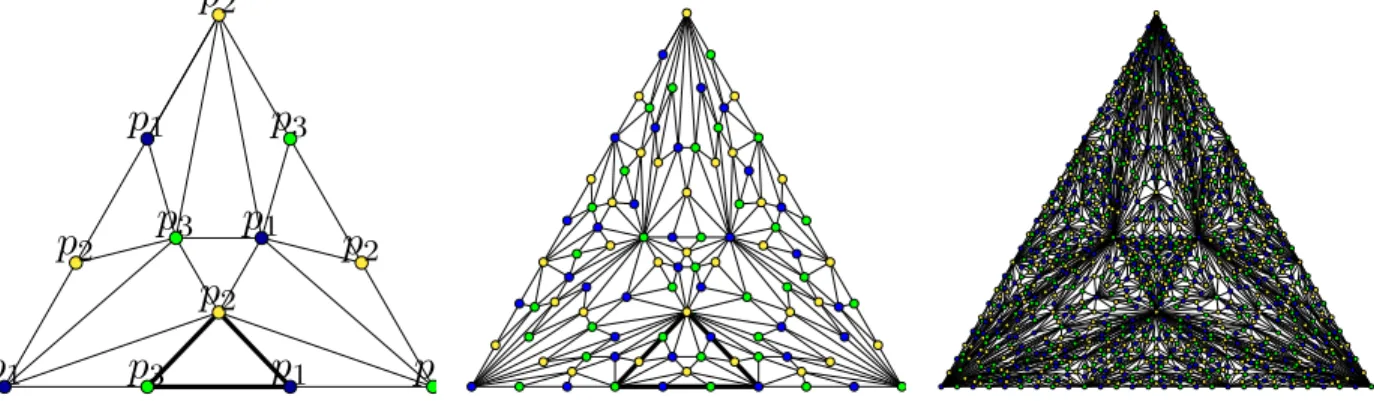
The properties that characterize the write_snapshot() operation are represented in the first picture of Figure 2, for the case of three processes. In the topology parlance, this picture represents a simplicial complex,, i.e., a family of sets closed under containment. Each set, which is called a simplex, represents the views of the processes after accessing the IS object. The vertices are0-simplexes of size one; edges are 1-simplexes, of size two; triangles are of size three (and so on). Each vertex is associated with a process pi, and is labeled with smi(the view piobtains from the object).
The highlighted2-simplex in the figure represents a run where p1and p3access the object concurrently, both get
the same views seeing each other, but not seeing p2, which accesses the object later, and gets back a view with the 3
values written to the object. But p2can’t tell the order in which p1and p3 access the object; the other two runs are
These two runs are represented by the2-simplexes at the bottom corners of the first picture. Thus, the vertices at the corners of the complex represents the runs where only one process piaccesses the object, and the vertices in the edges
connecting the corners represent runs where only two processes access the object. The triangle in the center of the complex, represents the run where all three processes access the object concurrently, and get back the same view.
p
1p
1p
3p
2p
3p
2p
3p
1p
3p
2p
2p
1Figure 2: One, two and three rounds in the iterated write-snapshot (IWS) model
Hence, the state of an execution after the first round (with which is associated the write-snapshot object WS[1]) is represented by one of the internal triangles (e.g., the one discussed previously that is represented by the bold triangle in the pictures). Then, the state of that execution after the second round (with which is associated the write-snapshot object WS[2]) is represented by one of the small triangles inside the bold triangle. Etc. More generally, as shown in Figure 2, one can see that, in the write-snapshot iterated model, at every round, a new complex is constructed recursively by replacing each simplex by a one-round complex.
4.3
A recursive write-snapshot algorithm
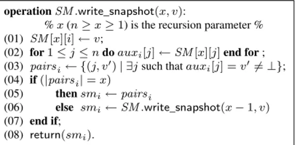
Figure 3 presents a read/write algorithm that implements the write_snapshot() operation. Interestingly, this algorithm is recursive [12, 22]. A proof can be found in [12]. To allow for a recursive formulation, an additional recursion parameter is used. More precisely, in a round r, a process invokes MS .write_snapshot(n, v) where the initial value of the recursion parameter is n and SM stands for WS[r].
SM is a shared array of size n (initialized to[⊥, . . . , ⊥] and such that each SM [x] is an array of n 1WnR atomic registers. The atomic register SM[x][i] can be read by all processes but written only by pi.
Let us consider the invocation SM .write_snapshot(x, v) issued by pi. Process pifirst writes SM[x][i] and reads
(not atomically) the array SM[x][1..n] that is associated with the recursion parameter x (lines 01-02). Then, pi
computes the set of processes that have already attained the recursion level x (line 03; let us note that recursion levels are decreasing from n to n− 1, etc.). If the set of processes that have attained the recursion level x (from pi’s point of
view) contains exactly x processes, pireturns this set as a result (lines 04-05). Otherwise less than x processes have
attained the recursion level x. In that case, pi recursively invokes SM .write_snapshot(x − 1) (line 06) in order to
attain and stop at the recursion level y attained by y processes.
The cost of a shared memory distributed algorithm is usually measured by the number of shared memory accesses, called step complexity. The step complexity of pi’s invocation is O(n(n − |smi| + 1)).
4.4
Iterative model vs recursive algorithm
It is interesting to observe that the iterative structure that defines the IWS model and the recursion-based formulation of the previous algorithm are closely related notions. In one case iterations are at the core of the model while in the other case recursion is only an algorithmic tool. However, the runs of a recursion-based algorithm are of an iterated nature: in each iteration only one array of registers is accessed, and the array is accessed only in this iteration.
operation SM .write_snapshot(x, v):
% x (n≥ x ≥ 1) is the recursion parameter % (01) SM[x][i] ← v;
(02) for1 ≤ j ≤ n do auxi[j] ← SM [x][j] end for ;
(03) pairsi← {(j, v′) | ∃j such that auxi[j] = v′6= ⊥};
(04) if(|pairsi| = x)
(05) then smi← pairsi
(06) else smi← SM .write_snapshot(x − 1, v)
(07) end if; (08) return(smi).
Figure 3: Recursive write-snapshot algorithm (code for pi)
5
Enriching a system with a failure detector
The concept of a failure detector This concept has been introduced by Chandra and Toueg [14] (see [46] for an introductory survey). Informally, a failure detector is a device that provides each process pi with information about
process failures, through a local variable fdi that pican only read. Several classes of failure detectors can be defined
according to the kind and the quality of the information on failures that has to be delivered to the processes.
Of course, a non-trivial failure detector requires that the system satisfies additional behavioral assumptions in order to be implemented. The interested reader will find such additional behavioral assumptions and corresponding algorithms implementing failure detectors of several classes in chapter 7 of [47].
An example One of the most known failure detectors is the eventual leader failure detector denotedΩ [13]. This failure detector is fundamental because it encapsulates the weakest information on failures that allows consensus to solved in a base read/write asynchronous system.
The output provided by Ω to each (non crashed) process pi is such that fdi always contains a process identity
(validity). Moreover, there is a finite time τ after which all local failure detector outputs fdi contains forever the same
process identity and it is the identity of a correct process (eventual leadership). The time τ is never explicitly know by the processes. Before τ , there is an anarchy period during which the local failure detector outputs can be arbitrary. A result As indicated, the consensus problem cannot be solved in the base read read/write system [39] but can be solved as soon as this system is enriched withΩ.
On another side (see Theorem 1), the base shared memory model and the IWS model have the same wait-free computability power bounded tasks. Hence a natural question: Is this computability power equivalence preserved when both models are enriched with the same failure detector? Somehow surprisingly, the answer to this question is negative. More precisely, we have the following.
Theorem 2 [44] For any failure detector FD and bounded task T , if T is wait-free solvable in the model IWS enriched with FD, then T is wait-free solvable in the base shared memory model without failure detector.
Intuitively, this negative result is due to the fact that the IWS model is too much structured to benefit from the help of a failure detector.
How to circumvent the previous negative result A way to circumvent this negative result consists in “embedding” (in some way) the failure detector inside the write_snapshot) operation. More precisely, the infinite sequence of invocations WS[1].write_snapshot), WS [2].write_snapshot), etc., issued by any process pihas to satisfy an additional
property that depends on the corresponding failure detector. This approach has given rise to the IRIS model described in [45].
6
From the wait-free model to the adversary model
Adversaries are a very useful abstraction to represent subsets of executions of a distributed system. The idea is that, if one restricts the set of possible executions, the system should be able to compute more tasks. For example, the condition based approach [41] restricts the set of inputs of a task (and hence the corresponding executions), and allows to solve more tasks, or to solve tasks faster. Various adversaries have been considered in the past to model failure restrictions, as we shall now describe.
6.1
The notion of an adversary
In the wait-free model, any number of process can crash. In practice one sometimes estimates a bound t on how many processes can be expected to crash. However, often the crashes are not independent, due to processes running on the same core, or on the same subnetwork, for example.
Wait-freedom It is easy to see that wait-freedom is the least restrictive adversary, i.e., the adversary that contains all the (non-empty) subsets of processes, namely, the sets of processes that may be alive in some execution. Hence, a wait-free algorithm has to work whatever the number of process crashes.
t-Faulty process resilience The t-faulty process resilient failure model (also called t-threshold model) considers that, in any run, at most t processes may crash. Hence, the corresponding adversary is the set of all the sets of(n − t) processes plus all their supersets: for each such set, there are executions where the processes that do not crash consist of this set.
Cores and survivor sets The notion of t-process resilience is not suited to capture the case where processes fail in a dependent way. This has motivated the introduction of the notions of core and survivor set [37].
A core C is a minimal set of processes such that, in any run, some process in C does not fail. A survivor set S is a minimal set of processes such that there is a run in which the set of non-faulty processes is exactly S. Let us observe that cores and survivor sets are dual notions (any of them can be obtained from the other one).
Computability results of set agreement have been generalized from t-resilience to cores in [27]. A connection relating adversaries that are superset-closed (i.e.,(s ∈ A) ⇒ (∀s′: s ⊆ s′: s′ ∈ A)) and wait-freedom is presented
in [21].
It is easy to see that the notion of survivor sets is more general than the notion t-threshold resilience. It is also possible to see that more general notions failures are possible:
Adversaries The most general notion of adversary with respect to failure dependence has been introduced in [16]. An adversary A is a set of sets of processes. It states that an algorithm solving a task must terminate in all the runs whose the corresponding set of correct processes is (exactly) a set of A.
As an example, Let us considers a system with four processes denoted p1, ..., p4. The set A= {{p1, p2},{p1, p4},{p1, p3, p4}}
defines an adversary. An algorithm A-resiliently solves a task if it terminates in all the runs where the set of correct processes is exactly either{p1, p2} or {p1, p4} or {p1, p3, p4}. This means that an A-resilient algorithm is not required
to terminate in an execution in which the set of correct processes is exactly the set{p3, p4} or the set {p1, p2, p3}.
Adversaries are more general than the notion of survivor sets (this is because when we build the adversary corre-sponding to a set of survivor sets, due the “minimality” feature of each survivor set, we have to include all its supersets in the corresponding adversary).
On progress conditions It is easy to see that an adversary can be viewed as a liveness property that specifies the crash patterns in which the correct processes must progress. The interested reader will find more developments on progress conditions in [20, 21, 36, 48].
6.2
Simulating the snapshot model in the iterated model
The iterated write-snapshot model (IWS) has been presented in Section 4 where we have seen that the base read/write (or snapshot) shared memory model and the IWS model are equivalent from a wait-free (bounded) task solvability point of view [9].
This section shows that this equivalence remains true when wait-freedom is replaced by an adversary-based progress condition. To that end, this section presents the simulation of the snapshot memory model in a simple variant of the IWS model where wait-freedom is replaced by the adversary defined by survivor sets. This simulation is from [23].
The snapshot-based algorithm LetA be the snapshot-based algorithm we want to simulate. We assume without loss of generality that it is a full information algorithm, i.e., each time a process writes, it writes its full local state. Initially, each process pihas an input value denoted inputi. Then, each process alternates between writing its state in
the shared memory, taking a snapshot of the shared memory and taking this snapshot as its new local state.
The algorithmA solves a task with respect to an adversary A if each correct process decides a value based on its current local state in every run that is fair with respect to A (which means that each time a process takes a snapshot it reads new values written by processes of a survivor set of the adversary A). This means that as in [23], given a snapshot object WS , a process writes it only once but can repeatedly invokes WS .snapshot() until it sees new values from a survivor set of A.
Given a local state of a process, we assume that the algorithmA has a predicate undecided(state) and a decision function decide(state). Once a process has decided, its predicate undecided(state) remains forever false. The kth snapshot issued by piis denoted snapshot(k, i) and its kth write is denoted write(k, i).
As it does not lead to confusion, we use “pi” to denote both the simulated process and the process that simulates
it.
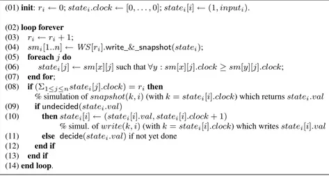
Simulation: the operation WS[r].write_&_snapshot(v) This is the simulation operation that allows processes to coordinate and communicate. When a process piinvokes it, it does the following. The value v is written in WS[r][i]
and piwaits until the set of processes that have written into WS[r] contains a survivor set of A. When this happens,
a snapshot of WS[r] is taken and returned. To simplify the presentation we consider that the snapshot value that is returned is an array sm[1..n].
(01) init: ri← 0; statei.clock← [0, . . . , 0]; statei[i] ← (1, inputi).
(02) loop forever (03) ri← ri+ 1;
(04) smi[1..n] ← WS [ri].write_&_snapshot(statei);
(05) foreach j do
(06) statei[j] ← sm[x][j] such that ∀y : sm[x][j].clock ≥ sm[y][j].clock;
(07) end for;
(08) if(Σ1≤j≤nstatei[j].clock) = rithen
% simulation of snapshot(k, i) (with k = statei[i].clock) which returns statei.val
(09) if undecided(statei.val)
(10) then statei[i] ← (statei[i].val, statei[i].clock + 1)
% simul. of write(k, i) (with k = statei[i].clock) which writes statei[i].val
(11) else decide(statei.val) if not yet done
(12) end if (13) end if (14) end loop.
Figure 4: The iterated simulation for adversary A (code for pi)
Simulation: local variables A process pimanages the following local variables.
• statei[1..n] is an array of pairs such that statei[x].clock is a clock value (integer) that measures the progress of
pxas know by piand statei[x].val is the corresponding local state of px; statei[i].val is initialized to inputi
(the input value of pi), the initial values of the other statei[j].val are irrelevant. The notation statei.clock is
used to denote the array[statei[1].clock, . . . , statei[n].clock] and similarly for statei.val.
Simulation: behavior of a process During a round r, the behavior of a process piis made up of two parts.
• First piwrites its current local state stateiin WS[r] and saves in smithe view of the global state it obtains for
that round (line 04). Then (lines 05-07) picomputes its new local state as follows: it saves in statei[j] the most
recent local state of pjit knows (“most recent” refers to the clock values that measures pjprogress).
• Then the simulation pistrives for making the simulation of the simulated process to progress.
The quantityΣ1≤j≤nstatei[j].clock represents the current date of the global simulation from pi’s point of view.
If this date is different from pi’s current round number r, then piis late (as far as its round number is concerned)
and it consequently proceeds to the next simulation round in order to catch up. (The proof shows that the predicateΣ1≤j≤nstatei[j].clock ≤ r remains invariant.)
IfΣ1≤j≤nstatei[j].clock = r, the round number is OK for pito simulate the invocation snapshot(k, i) of the
simulated process where k= statei[i].clock. The corresponding value that is returned is statei.val.
Then, if its state is undecided (line 09), pi makes the simulation progress by simulating write(k, i) where
k= statei[i].clock + 1 and the value written is statei[i].val (line 10).
If the state of pican allow for a decision, pidecides if not yet done (line 11). Let us notice that, as soon as a
process pi has decided, it continues looping (this is necessary to prevent permanent blocking if pi belongs to
survivor sets) but its local clock is no longer increased in order to allow the correct processes to decide. A proof of this simulation can be found in [23]. It is based on the observation that if for two processes the round number is OK, then theirs state variables agree.
7
Simulating adversary models in the wait-free model
The simulation of Section 6.2 showed that the same tasks can be solved in the iterated write-snapshot (IWS) model and in the base read/write (or snapshot) shared memory model, in the presence of failures. Namely, considering adversaries defined by survivor sets, a task can be solved in the IWS model under some adversary if and only if it can be solved in the base model, under the same adversary. As we have seen, the simplest adversary is the wait-free adversary. So it would be nice to reduce questions about task solvability under other adversaries, to the wait-free case. This is exactly what the BG simulation [10] and its variants (e.g. [19, 33, 34]) allow.
BG simulation and its variants Let us consider an algorithmA that is assumed to solve a task T in an asynchronous read/write shared memory system made up of n processes, and where any subset of at most t processes may crash. Given algorithmA as input, the BG simulation is an algorithm that solves T in an asynchronous read/write system made up of t+ 1 processes, where up to t processes may crash. Hence, the BG simulation is a wait-free algorithm.
The BG simulation has been used to prove solvability and unsolvability results in crash-prone read/write shared memory systems. It works only for a particular class of tasks called colorless tasks. These are the tasks where, if a process decides a value, any other process is allowed to decide the very same value, and if a process has an input value v, then any other processes can exchange its own input by v. Thus, for colorless tasks, the BG simulation characterizes t-resilience in terms of wait-freedom, and it is not hard to see that the same holds for any other adversary (defined by survivor sets).
As an example, let us assume thatA solves consensus, despite up to t = 1 crash, among n processes in a read/write shared memory system. TakingA as input, the BG simulation builds a (t + 1)-process (i.e., 2-process) algorithm A′
that solves consensus despite t = 1 crash, i.e., wait-free. But, we know that consensus cannot be wait-free solved in a crash-prone asynchronous system where processes communicate by accessing shared read/write registers only
[17, 25, 39] in particular if it is made up of only two processes. It then follows that, whatever the number n of processes the system is made up of, there is no1-resilient consensus algorithm.
The BG simulation algorithm has been extended to work with general tasks (called colored tasks) [19, 33] and for algorithms that have access to more powerful communication objects (e.g., [34] that extends the BG simulation to the 0/1-exclusion objects defined in [18]).
The idea of the BG simulation LetA be an algorithm that solves a colorless decision task in the t-resilient model for n processes. The basic aim is to design a wait-free algorithmA′that simulatesA in a model with t + 1 processes.
A simulated process is denoted pj, while a simulator process is denoted qj, with1 ≤ j ≤ n.
Each simulator qjis given the code of every simulated process p1, . . . , pn. It manages n threads, each one
associ-ated with a simulassoci-ated process, and locally executes these threads in a fair way (e.g., using a round-robin mechanism). It also manages a local copy memiof the snapshot memory mem shared by the simulated processes. The code of
a simulated process pj contains invocations of mem[j].write() and of mem.snapshot(). These are the only
opera-tions used by the processes p1, . . . , pn to cooperate. So, the core of the simulation is the design of algorithms that
describe how a simulator qisimulates these operations. These simulation algorithms are denoted sim_writei,j(), and
sim_snapshoti,j().
The safe agreement object type is at the core of the BG simulation. It provides each simulator qi with two
op-erations, denoted sa_propose(v) and sa_decide(), that qi can invoke at most once, and in that order. The operation
sa_propose(v) allows qito propose a value v while sa_decide() allows it to decide a value. The properties satisfied by
an object of the type safe agreement are the following.
• Termination. If no simulator crashes while executing sa_propose(v), then any correct simulator that invokes sa_decide() returns from that invocation.
• Agreement. At most one value is decided. • Validity. A decided value is a proposed value.
BG simulation and iterated models Simple implementations of the safe agreement type are described in [10, 35]. We introduce here an alternative implementation, that works in the iterated write-snapshot model (IWS). Actually, an implementation of sa_propose() and sa_decide() needs two iterations of the base IWS model. We hope this example illustrates the benefits of programming in the iterated model. As the safe agreement object is at the core of the BG simulation, doing so connects the BG simulation with the “iterated model” research line.
As seen in Section 4.1 the semantics of the write_snapshot() operation is defined by the properties Self-inclusion, Containment, Immediacy, and Termination which have been described in that section.
operation sa_propose(v): (01) sm1
i ← WS [1].write_snapshot(v);
(02) sm2
i ← WS [2].write_snapshot(sm1i).
Figure 5: Operation sa_propose(v) in the iterated model (code for qi)
The two underlying write-snapshot objects used to implement a safe agreement object are denoted WS[1] and WS[2]. An algorithm implementing the safe agreement operation sa_propose(v) is described in Figure 5. When a simulator qiinvokes sa_propose(v) it writes v into the first write-snapshot object WS [1] and stores the result in a local
variable sm1i (line 01). It then writes this result in the second write-snapshot object, and stores the result in sm 2 i (line
02).
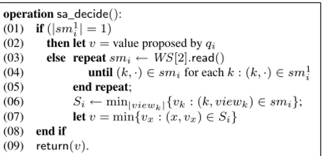
An algorithm implementing the sister operation sa_decide() is described in Figure 6. When a simulator qiinvokes
sa_decide(), it inspects sm1
i to find out how many processes it saw in the first iteration of its sa_propose() invocation.
If the set sm1
i is such that|sm 1
i| = 1, it contains only the value proposed by qi, and qidecides then this value (lines
01, 02 and 09).
Otherwise, in addition to the value proposed by qi, sm1i contains values proposed by other processes. This means
operation sa_decide(): (01) if(|sm1
i| = 1)
(02) then let v= value proposed by qi
(03) else repeat smi← WS [2].read()
(04) until(k, ·) ∈ smifor each k: (k, ·) ∈ sm1i
(05) end repeat;
(06) Si← min|viewk|{vk: (k, viewk) ∈ smi};
(07) let v= min{vx: (x, vx) ∈ Si}
(08) end if (09) return(v).
Figure 6: Operation sa_decide() in the iterated model(code for qi)
In this statement qirepeatedly reads the second write-snapshot object WS[2] (line 031) and stores the result in smi,
until it sees that all processes in sm1
i have written a value to it. If no simulator crashes while executing sa_propose(),
this wait statement terminates and (if it does not crash) qireturns from its invocation of sa_decide(). This is precisely
the termination property of the safe consensus object type.
Once qiexits the wait statement, its local variable smiincludes a pair(k, viewk), for each pkthat appears in sm 1 i,
and viewkcorresponds to the value written by pkin the second iteration. Namely, viewk is the view of pkin the first
iteration (a set of pairs). Let Sibe equal to the viewk with the smallest size such that the pair(k, viewk) ∈ smi(line
06):
Si← min
|viewk|
{viewk : (k, viewk) ∈ smi}.
The main point is that any two simulators qi, qj compute the same set: Si = Sj. Thus, they can decide on any
deterministically chosen value from Si, say the smallest proposed value present in Si(line 07):
v← min{vx: (x, vx) ∈ Si}.
8
Conclusion
This paper has presented an introductory survey of recent advances in asynchronous shared memory models where processes can commit unexpected crash failures. To that end the base snapshot model and iterated models have been presented. As far as resilience is concerned, the wait-free model and the adversary model have been discussed. Moreover, the essence of the Borowsky-Gafni’s simulation has been described. It is hoped that this survey will help a larger audience of the distributed computing community to understand the power, subtleties and limits of crash-prone asynchronous shared memory models.
References
[1] Afek Y., Attiya H., Dolev D., Gafni E., Merritt M. and Shavit N., Atomic Snapshots of Shared Memory. Journal of the ACM, 40(4):873-890, 1993.
[2] Attiya H., Rachman O., Atomic Snapshots in O(n log n) Operations. SIAM Journal of Computing, 27(2): 319–340, 1998.
[3] Afek Y., Gafni E., Rajsbaum S., Raynal M. and Travers C., The k-Simultaneous Consensus Problem. Distributed Computing, 22(3): 185-195, 2010.
[4] Anderson J., Multi-writer Composite Registers. Distributed Computing, 7(4):175-195, 1994.
[5] Attiya H., Bar-Noy A. and Dolev D., Sharing Memory Robustly in Message Passing Systems. Journal of the ACM, 42(1):121-132, 1995.
1Recall that, as in the simulation of Section 6.2, we are assuming that, although writing a write-snapshot object of the IWS model is done
only once, it can be read many times. Hence, we assume here an operation WS[2].read() that returns asynchronously all the pairs presents in the write-snapshot WS[2].
[6] Attiya H., Bar-Noy A., Dolev D., Peleg D. and Reischuk R., Renaming in an Asynchronous Environment. Journal of the ACM, 37(3):524-548, 1990.
[7] Attiya H., Guerraoui R. and Ruppert E., Partial Snapshot Objects. Proc. 20th ACM Symposium on Parallel Architectures and Algorithms (SPAA’08), ACM Press, pp. 336-343, 2008.
[8] Borowsky E. and Gafni E., Immediate Atomic Snapshots and Fast Renaming. Proc. 12th ACM Symposium on Principles of Distributed Computing (PODC’93), pp. 41-51, 1993.
[9] Borowsky E. and Gafni E., A Simple Algorithmically Reasoned Characterization of Wait-free Computations. Proc. 16th ACM Symposium on Principles of Distributed Computing (PODC’97), ACM Press, pp. 189-198, 1997.
[10] Borowsky E., Gafni E., Lynch N. and Rajsbaum S., The BG Distributed Simulation Algorithm. Distributed Computing, 14(3):127-146, 2001. [11] Charron-Bost B. and Schiper A., The Heard-Of model: computing in distributed systems with benign faults. Distributed Computing, 22(1),
49–71, 2009.
[12] Castañeda A., Rajsbaum S. and Raynal M., The Renaming Problem in Shared Memory Systems: an Introduction. Computer Science Review, to appear, 2011.
[13] Chandra T., Hadzilacos V. and Toueg S., The Weakest Failure Detector for Solving Consensus. Journal of the ACM, 43(4):685-722, 1996. [14] Chandra T. and Toueg S., Unreliable Failure Detectors for Reliable Distributed Systems. Journal of the ACM, 43(2):225-267, 1996. [15] Chaudhuri S., More Choices Allow More Faults: Set Consensus Problems in Totally Asynchronous Systems. Information and Computation,
105(1):132-158, 1993.
[16] Delporte-Gallet C., Fauconnier H., Guerraoui R. and Tielmann A., The Disagreement Power of an Adversary. Proc. 23th Int’l Symposium on Distributed Computing (DISC’09), Springer-Verlag LNCS #5805, pp. 8-21, 2009.
[17] Fischer M.J., Lynch N.A. and Paterson M.S., Impossibility of Distributed Consensus with One Faulty Process. Journal of the ACM, 32(2):374-382, 1985.
[18] Gafni E., The01-Exclusion Families of Tasks. Proc. 12th In’l Conference on Principles of Distributed Systems (OPODIS’08, Springer Verlag LNCS #5401, pp. 246-258, 2008.
[19] Gafni E., The Extended BG Simulation and the Characterization of t-Resiliency. Proc. 41th ACM Symposium on Theory of Computing (STOCÕ09), ACM Press, pp. 85-92, 2009.
[20] Gafni E. and Kuznetsov P., Turning Adversaries into Friends: Simplified, Made Constructive and Extended. Proc. 14th Int’l Conference on Principles of Distributed Systems (OPODIS’10), Springer-Verlag, #LNCS 6490, pp. 380-394, 2010.
[21] Gafni E. and Kuznetsov P., RelatingL-Resilience and and Wait-freedom with Hitting Sets. Proc. 12th Int’l Conference on Distributed Computing and Networking (ICDCN’11), Springer-Verlag, #LNCS 6522, pp. 191-202, 2011.
[22] Gafni E. and Rajsbaum S., Recursion in Distributed Computing. Proc. 12th Int’l Symposium on Stabilization, Safety, and Security of Dis-tributed Systems (SSS’10), Springer-Verlag, #LNCS 6366, pp. 362-376, 2010.
[23] Gafni E. and Rajsbaum S., Distributed Programming with Tasks. Proc. 14th Int’l Conference on Principles of Distributed Systems (OPODIS’10), Springer-Verlag, #LNCS 6490, pp. 205-218, 2010.
[24] Guerraoui R. and Raynal M., From Unreliable Objects to Reliable Objects: the Case of atomic Registers and Consensus. 9th Int’l Conference on Parallel Computing Technologies (PaCT’07), Springer Verlag LNCS LNCS #4671, pp. 47-61, 2007.
[25] Herlihy M.P., Wait-Free Synchronization. ACM Transactions on Programming Languages and Systems, 13(1):124-149, 1991.
[26] Herlihy M.P., Luchangco V. and Moir M., Obstruction-free Synchonization: Double-ended Queues as an Example. Proc. 23th Int’l IEEE Conference on Distributed Computing Systems (ICDCS’03), pp. 522-529, 2003.
[27] Herlihy M. P. and Rajsbaum S., The Topology of Shared Memory Adversaries. Proc. 29th ACM Symposium on Principles of Distributed Computing (PODC’10), ACM Press, pp. 105-113, 2010.
[28] Herlihy M.P. and Rajsbaum S., Concurrent Computing and Shellable Complexes. Proc. 24th Int’l Symposium on Distributed Computing (DISC’10), Springer Verlag LNCS #6343, pp. 109-123, 2010.
[29] Herlihy M.P., Rajsbaum S., and Tuttle, M., Unifying Synchronous and Asynchronous Message-Passing Models. Proc. 17th ACM Symposium on Principles of Distributed Computing (PODC’98), ACM Press, pp. 133–142, 1998.
[31] Herlihy M.P. and Wing J.L., Linearizability: a Correctness Condition for Concurrent Objects. ACM Transactions on Programming Languages and Systems, 12(3):463-492, 1990.
[32] Imbs D. and Raynal M., Help when Needed, but no More: Efficient Read/Write Partial Snapshot. Proc. 23th Int’l Symposium on Distributed Computing (DISC’09), Springer-Verlag LNCS #5805, pp. 142-156, 2009.
[33] Imbs D. and Raynal M., Visiting Gafni’s Reduction Land: from the BG Simulation to the Extended BG Simuation. Proc. 11th Int’l Symposium on Stabilization, Safety, and Security of Distributed Systems (SSS’09), Springer-Verlag LNCS #5873, pp. 369-383, 2009.
[34] Imbs D. and Raynal M., The Multiplicative Power of Consensus Numbers. Proc. 29th ACM Symposium on Principles of Distributed Com-puting (PODC’10), ACM Press, pp. 26-35, 2010.
[35] Imbs D. and Raynal M., A Liveness Condition for Concurrent Objects: x-Wait-freedom. To appear in Concurrency and Computation: Practice and experience, 2011.
[36] Imbs D., Raynal M. and Taubenfeld G., On Asymmetric Progress Conditions. Proc. 29th ACM Symposium on Principles of Distributed Computing (PODC’10), ACM Press, pp. 55-64, 2010.
[37] Junqueira F. and Marzullo K., Designing Algorithms for Dependent Process Failures. Future Directions in Distributed Computing, Springer-Verlag, #LNCS 2584, pp. 24-28, 2003.
[38] Lamport. L., On Interprocess Communication, Part 1: Basic formalism, Part II: Algorithms. Distributed Computing, 1(2):77-101,1986. [39] Loui M.C., and Abu-Amara H.H., Memory Requirements for Agreement Among Unreliable Asynchronous Processes. Par. and Distributed
Computing: vol. 4 of Advances in Comp. Research, JAI Press, 4:163-183, 1987.
[40] Moses Y. and Rajsbaum S., A Layered Analysis of Consensus. SIAM Journal Computing 31(4): 989-1021, 2002.
[41] Mostéfaoui A., Rajsbaum S. and Raynal M., Conditions on Input Vectors for Consensus Solvability in Asynchronous Distributed Systems. Journal of the ACM, 50(6):922-954, 2003.
[42] Neiger G., Set Linearizability. Brief Announcement, Proc. 13th ACM Symposium on Principles of Distributed Computing (PODC’94), ACM Press, pp. 396, 1994.
[43] Rajsbaum S., Iterated Shared Memory Models. Proc. 9th Latin American Symposium Theoretical Informatics (LATIN’10), Springer Verlag LNCS #6034, pp. 407-416, 2010.
[44] Rajsbaum S., Raynal M. and Travers C., An Impossibility about Failure Detectors in the Iterated Immediate Snapshot Model. Information Processing Letters, 108(3):160-164, 2008.
[45] Rajsbaum S., Raynal M. and Travers C., The Iterated Restricted Immediate Snapshot (IRIS) Model. 14th Int’l Computing and Combinatorics Conferernce (COCOON’08), Springer-Verlag LNCS 5092, pp.487-496, 2008.
[46] Raynal M., Failure Detectors for Asynchronous Distributed Systems: an Introduction. Wiley Encyclopdia of Computer Science and Engi-neering, Vol. 2, pp. 1181-1191, 2009.
[47] Raynal M., Communication and Agreement Abstractions for Fault-Tolerant Asynchronous Distributed Systems. Morgan & Claypool Pub-lishers, 251 pages, 2010 (ISBN 978-1-60845-293-4).
[48] Taubenfeld G., The Computational Structure of Progress Conditions. Proc. 24th Int’l Symposium on Distributed Computing (DISC’10), Springer Verlag LNCS #6343, pp. 221-235, 2010.