Lazy Reachability Analysis in Distributed Systems

HAL Id: hal-01699311

https://hal.archives-ouvertes.fr/hal-01699311

Submitted on 2 Feb 2018

HAL is a multi-disciplinary open access

archive for the deposit and dissemination of

sci-entific research documents, whether they are

pub-lished or not. The documents may come from

teaching and research institutions in France or

abroad, or from public or private research centers.

L’archive ouverte pluridisciplinaire HAL, est

destinée au dépôt et à la diffusion de documents

scientifiques de niveau recherche, publiés ou non,

émanant des établissements d’enseignement et de

recherche français ou étrangers, des laboratoires

publics ou privés.

To cite this version:

Loïg Jezequel, Didier Lime.

Lazy Reachability Analysis in Distributed Systems.

27th

In-ternational Conference on Concurrency Theory (CONCUR 2016), Aug 2016, Québec, Canada.

�10.4230/LIPIcs.CONCUR.2016.17�. �hal-01699311�

Loïg Jezequel

and Didier Lime

1 Université de Nantes, IRCCyN UMR CNRS 6597, France

Loig.Jezequel@irccyn.ec-nantes.fr

2 École Centrale de Nantes, IRCCyN UMR CNRS 6597, France

Didier.Lime@ec-nantes.fr

Abstract

We address the problem of reachability in distributed systems, modelled as networks of finite automata and propose and prove a new algorithm to solve it efficiently in many cases. This algorithm allows to decompose the reachability objective among the components, and proceeds by constructing partial products by lazily adding new components when required. It thus con-structs more and more precise over-approximations of the complete product. This permits early termination in many cases, in particular when the objective is not reachable, which often is an unfavorable case in reachability analysis. We have implemented this algorithm in a first prototype and provide some very encouraging experimental results.

1998 ACM Subject Classification D.2.4 Software/Program Verification

Keywords and phrases Reachability analysis, compositional verification, automata

Digital Object Identifier 10.4230/LIPIcs.CONCUR.2016.17

1

Introduction

As distributed systems become more and more pervasive, the need for the verification of their correctness increases accordingly. The problem of verifying that some particular state of the system is reachable is a cornerstone in this endeavour. Yet even this simple problem is challenging in a distributed context, due to the exponential growth of the state-space of the system with the number of components, a problem often referred to as “state explosion”.

To alleviate this issue several approaches have been proposed in the last two decades. In particular, partial order techniques, which allow to explore only part of the state-space while preserving completeness, have proved to be an efficient approach [12] and are implemented in some state-of-the-art tools, including LoLA [15]. Another technique called partial model-checking has been proposed in [1], which consists in incrementally quotienting temporal logic formulas by incorporating the behaviours of individual processes into that formula. This leads to a compositional verification scheme that has been recently extended and implemented in the PMC tool on top of the CADP toolbox [14]. This idea to incrementally take into account components of distributed systems is also present in works on compositional minimization [9, 6] and modular model checking [10, 7]. Recently, the IC3 algorithm [3] has been proposed to address the safety / reachability issue, with very promising results. This algorithm incrementally generates more and more precise over-approximations of the reachability relation, by computing stronger and stronger inductive assertions using SAT solving [3] or SMT solving [4]. Similar ideas of incremental refinements were also successfully used in AI planning [2, 11].

A common high-level scheme in the partial model-checking approach, the IC3 approach, and the hierarchical planning approach is to incrementally compute more and more precise approximate objects until sufficient precision permits to conclude. We propose a new approach

also based on this scheme. Contrarily to IC3, we deliberately use the classical tools of explicit state space exploration in finite automata-based models, with the motivation of ultimately combining our technique with some of the most successful improvements of these tools, like partial-order reduction techniques, and with well-known extensions to more expressive models like timed automata. In contrast to the partial model-checking approach, we take advantage of the simplicity of the reachability property we study, and adopt a lower-level approach, by focusing on the individual components of the system and their fine interactions.

Our contribution in this paper is therefore the following: first an algorithm, which projects a reachability property on the individual components, then lazily adds components to the projections and merges them together as interactions that are meaningful to the reachability property are discovered. We provide full proofs for completeness, soundness, and termination. Second, we report on a prototype implementation that permits a first evaluation of our algorithm. We have compared these performances with LoLA.

The paper is organized as follows: in Section 2 we give the basic definitions upon which our algorithm is built. In Section 3, we describe our algorithm and prove it. In Section 4 we report on experimental results, and we conclude in Section 5.

2

Preliminary definitions

2.1 LTSs and their products

We focus on labelled transition systems, synchronized on common actions, as models.

IDefinition 1. A labelled transition system (LTS) is a tuple L = (S, ι, T, Σ, λ) where S is a

non-empty finite set of states, ι ∈ S is an initial state, Σ is an alphabet of transition labels,

T ⊆ S × S is a finite set of transitions, and λ : T → Σ is a transition labeling function.

By a slight abuse of notations, we also denote by Σ(L) the set of labels of L and by λ(L) the set of labels effectively associated to at least one transition in L.

IDefinition 2. In such an LTS, a path is a sequence of transitions π = t1. . . tn such that: ∀1 ≤ k ≤ n, tk _{= (s}k_{, s}k+1_{) ∈ T and s}1_{= ι. In this case we say that π reaches s}n+1_{. A state}

s is said to be reachable if there exists a path that reaches s.

IDefinition 3. We say that two LTSs L1= (S1, ι1, T1, Σ1, λ1) and L2= (S2, ι2, T2, Σ2, λ2)

are isomorphic if and only if there exists two bijections fS : S1→ S2 and fT : T1→ T2 so

that: fS(ι1) = ι2, and ∀s1, s01∈ S1, (s1, s01) ∈ T1iff (fS(s1), fS(s01)) ∈ T2, and λ1((s1, s01)) = λ2((fS(s1), fS(s01))).

Our systems are built as parallel compositions of multiple LTSs.

IDefinition 4. Let L1, . . . , Ln be LTSs such that ∀1 ≤ i ≤ n, Li = (Si, ιi, Ti, Σi, λi). The

compound system L1 k . . . k Ln is the LTS (S, ι, T, Σ, λ) such that S = S1 × · · · × Sn,

ι = (ι1, . . . , ιn), Σ = Σ1∪ · · · ∪ Σn, and t = ((s1, . . . , sn), (s01, . . . , s0n)) ∈ T with λ(t) = σ if

and only if ∀1 ≤ i ≤ n if σ ∈ Σi then ti= (si, s0i) ∈ Ti and λi(ti) = σ else si= s0i.

Remark that (L1k L2) k L3, L1k (L2k L3), and L1k L2k L3are isomorphic (they are

identical up to renaming of states and transitions). It is thus possible to compute compound systems step by step, by adding LTSs to the composition one after the other.

IDefinition 5. Lid= (Sid, ιid, Tid, Σid, λid) with Sid = {id}, ιid= id, Tid = ∅, Σid= ∅, and

Remark that Lid can be considered as the neutral element for the composition of LTSs:

∀L, L k Lid and L are isomorphic. Also remark that for any LTS L, there is an LTS

containing only the initial state of L which is isomorphic to Lid. We denote it by id(L).

2.2 Partial products and reachability of partial states

IDefinition 6. An LTS L = (S, ι, T, Σ, λ) extends an LTS L0_{, noted L}0 _{v L, if and only}

if L0 is isomorphic to some LTS (S0, ι0, T0, Σ0, λ0) with S0⊆ S, T0 _{⊆ T, Σ}0_{⊆ Σ, ι = ι}0_{, and} λ0= λ|T0. If, moreover, S0 6= S, or T06= T, or Σ0 6= Σ, L is said to strictly extend L0, noted

L0

@ L.

We define ini(L) as the LTS containing only the initial state of L but, contrarily to id(L), with Σ(ini(L)) = Σ(L). Note that we clearly have ini(L) v L.

Given a set of LTSs, we now define partial products as products in which some parts of the LTSs, or possibly some LTSs altogether, are not used:

IDefinition 7. An LTS L0 is a partial product of a compound system L = L1k · · · k Ln if

there exists m LTSs L0_k

1, . . . , L

0

km (with {kj : j ∈ [1..m]} ⊆ [1..n]) such that L

0_{is isomorphic} to L0_k 1 k · · · k L 0 km and ∀j ∈ [1..m], L 0 kj v Lkj.

Note that in the algorithm we propose in Section 3, we will actually always have, by construction, ini(Lkj) v L

0

kj v Lkj, which implies that all three LTSs have the same alphabet.

We focus on solving particular reachability problems where one is interested in reaching partial states.

IDefinition 8. In a compound system L1k . . . k Ln we call any element from S1× · · · × Sn

a global state. A partial state is an element from (S1∪ {?}) × · · · × (Sn∪ {?}) \ {(?, . . . , ?)}.

We say that a partial state (s0₁, . . . , s0_n) concretises a partial state (s₁, . . . , s_n) if ∀i, s_i6= ? implies s0_i= s_i.

A partial state is therefore in some sense the specification of the set of global states that concretise it, i.e., that share the same values on dimensions not equal to ? in the partial state. We use partial states to specify our reachability objectives.

IDefinition 9. In a compound system L, a partial state is said reachable, if there exists a

reachable global state that concretises it. Given a set R of partial states, we call reachability

problem (RP_LR) the problem of deciding whether or not some element from R is reachable. Given a reachability problem RP_LR _{we denote by L}g the set of indices of the LTSs

involved in R: for each i ∈ Lg, there exists at least one partial state in which the element

corresponding to Li is not ?. In a reachability problem, if there exists a reachable global

state in L that concretises an element from R, we write L → R. If this is not the case, we write L 9 R.

We conclude this section by establishing two basic results on partial products of LTSs that will be instrumental in proving that our approach is sound and complete.

Lemma 10 formalizes the fact that, due to the synchronization by shared labels mechanism, removing an LTS from a product produces an over-approximation of the reachability property projected on the remaining LTSs.

ILemma 10. Let L = L1 k · · · k Ln be a compound system in which some global state

s = (s₁, . . . , s_n) is reachable. Let L0 be the partial product of L obtained by removing Li for

some i. Similarly, let s0 be the state of L0 obtained from s by removing the ith _{component s} i.

Then s0 is reachable in L0.

Lemma 11 works in the opposite direction to Lemma 10: If we can find a subset of the LTSs, in which we can reach some given state, and that does not make use of any label appearing in an LTS not in this subset – condition (i) –, then we can add the missing LTSs to get the full product, while still ensuring the reachability of our given state. The result we prove is actually a bit stronger: one can preserve the reachability found in a partial product of our subset of LTSs, provided that if some label appears on a transition in the partial product, then it is present in the alphabets of all the components of the partial product that can be extended into an LTS that uses this label – condition (ii). Condition (i) ensures that we do not add any synchronization constraint to existing transitions when adding new LTS, while condition (ii) does the same but when extending the LTSs already in the subset.

ILemma 11. Let L = L1 k · · · k Ln be a compound system. Let H ⊆ [1..n]. Suppose to

simplify the writing that H = [1..h] and let C = C1k · · · k Chbe a partial product of (ki∈HLi)

such that: (i) for all i 6∈ H, Σ(Li) ∩ λ(C) = ∅, and (ii) for all i ∈ H, Σ(Li) ∩ λ(C) ⊆ Σ(Ci).

If some global state s = (s₁, . . . , s_n) is reachable in C with path π then the global state

s∗= (s∗₁, . . . , s∗n) defined by s∗i = si if i ∈ H and s∗i is an arbitrary state of Li otherwise is

reachable in L with the same path from the state s0_{= (s}0

1, . . . , s0n) such that s0i is the initial

state of Li if i ∈ H and s0i = s∗i otherwise.

3

The Lazy Reachability Analysis Algorithm

In the following subsections, we present our algorithm. It makes use of the classical abstract list data-structure, with the usual operations: hd(), tl(), len() give respectively the head, tail, and length of a list. Operator : is the list constructor (prepend) and ++ is concatenation. rev() reverses a list. [ ] is the empty list and L[i] is the ith _{element of list L.}

Algorithm 1 Algorithm solving RP_LR _(Lg: indices of LTSs involved in R)

1: function Solve(L,R)

2: choose a partition {I₁, . . . , Ip} of Lg

3: ∀k ∈ [1..p], let IDk=ki∈Ikid(Li) and INIk=ki∈Ikini(Li).

4: Ls ← [([ ], (ID1, INI1, I1, ∅, I1), [ ]), . . . , ([ ], (IDp, INIp, Ip, ∅, Ip), [ ])]

5: Complete ← False

6: Consistent ← False

7: while not Complete or not Consistent do

8: Complete ← ∀k, Ls[k] is complete

9: if not Complete then

10: optional unless Consistent

11: mayHaveSol ← Concretise(Ls)

12: if not mayHaveSol then return False

13: end if

14: end option

15: end if

16: Consistent ← Ls is consistent

17: if not Consistent then

18: optional unless Complete

19: Merge(Ls) 20: end option 21: end if 22: end while 23: return True 24: end function

Algorithm 1 is the main function solving our reachability problems. It starts from a partition of the LTSs involved in the reachability objective. The idea here is to decompose

this objective and verify it separately on each involved component with the hope that they do not interact. List Ls has (initially) one element per part of the initial partition. Each of those elements is a list of tuples (A, C, I, J, K), described in details in the next subsection, that represent more and more concrete partial products (in the sense that they include more and more LTSs) of the system built around the LTSs in each partition, as we go towards the end of the list. In our algorithm, this list is walked along using the functional programming idiom of Huet’s Zipper by decomposing it in Left, the current element, and Right, but it could as well be represented as a big array with a current index, etc.

We start with partial products consisting of only the initial states of each involved LTSs. The algorithm then performs two main tasks: concretisation and merging.

3.1 Concretisation

Concretisation consists in extending the partial products in two different directions: by computing more and more states and transitions for a given number of LTSs, and by adding LTSs. The (indices of the) LTSs currently used in the products are in the set J , and those being added are in set K. Set I serves as a memory of the initial partition of LTSs involved in the objective. LTS C is the current partial product we have computed and A represents what we had computed at the previous level (before we added the LTSs in K).

Algorithm 2 Auxiliary function Concretise() for Algorithm 1

1: function Concretise(Ls)

2: choose k ∈ [0..len(Ls) − 1] such that Ls[k] is not complete

3: (Left, (A, C, I, J, K), Right) ← Ls[k]

4: if there exists C∗s.t. C @ C∗v (ki∈KLi) k A and C∗→ R|J ∪K then 5: choose such a C∗

6: N ← {i /∈ J ∪ K : Σ(Li) ∩ λ(C∗) 6= ∅}

7: case Right 6= [ ]

8: (_, C0, _, J0, K0) ← hd(Right)

9: Ls[k] ← ((A, C∗, I, J, K) : Left, (C∗, C0, I, J0, K0), tl(Right))

10: case Right = [ ] and N 6= ∅

11: choose ∅ ⊂ K0_{⊆ N}

12: Ls[k] ← ((A, C∗_{, I, J, K) : Left, (C}∗_{, k}

i∈J ∪K∪K0ini(Li), I, J ∪ K, K0), [ ])

13: case Right = [ ] and N = ∅

14: Ls[k] ← (Left, (A, C∗, I, J, K), [ ])

15: else

16: if Left = [ ] then return False

17: else

18: Right0_{← Forget((A, C, I, J, K) : Right)}

19: Ls[k] ← (tl(Left), hd(Left), Right0)

20: end if

21: end if

22: return True

23: end function

The goal of the Concretise() function (Algorithm 2) is to find a partial product reaching the objective and using only LTSs that are either in J or in K. This is what we call complete and is formalized as follows:

IDefinition 12 (Completeness). The tuple (Left, (A, C, I, J, K), Right) is complete if ∃C∗v C such that C∗→ R|J ∪K and {i /∈ J ∪ K : Σ(Li) ∩ λ(C∗) 6= ∅} = ∅.

To ensure completeness, we have to add LTSs that share actions with our current partial product: this is the role of the case in line 10.

LTS A serves as a limit as to what we are allowed to compute at a given level. If we need to compute more, because we cannot find the (partial) objective, we have to backtrack to the previous level to increase this limit (line 19). If we cannot backtrack (line 16), then we have explored the whole product only missing some components, so we have an over-approximation,

which implies that the property is false. If we successfully backtrack, and when we have extended again our partial product at that “lower” level, we can go forth again using the memory of what we had already computed (line 7).

Note the use of the Forget() function in line 19 that permits to “forget” part of that memory when we backtrack. This is useful if we are able to determine that we had made bad moves: for instance in the choice of the LTSs to add to the product. Many implementations of this function are possible provided they have the following property:

IProperty 13 (Good Forget() implementation). Let Lt be a list [(A1, C1, I1, J1, K1), . . . ,

(An, Cn, In, Jn, Kn)] of tuples. Then Forget(Lt) must be a list [(A01, C 0

1, I10, J10, K10), . . . ,

(A0m, C0m, Im0 , Jm0 , Km0 )] of tuples with 0 ≤ m ≤ n and f : [1..m] → [1..n] a non-decreasing

function, such that: A0₁= A1, J10 = J1,

∀j ∈ [1..m],

I_j0 = I1 (remark that, by construction, I1= I2= · · · = In),

∅ ⊂ K0 j⊆ (Jf (j)∪ Kf (j)) \ Jj0 C0_j v Cf (j) and kk∈J0 j∪K0jini(Lk) v C 0 jv (kk∈K0 j Lk) k A 0 j ∀j ∈ [2..m], A0j= C 0 j−1 J_j0 = J_j−10 ∪ K0 j−1

In some sens, a good Forget() implementation can be seen as a restriction of Lt to a subset of its elements. Each of these elements being itself restricted to a less concrete tuple (by taking subsets of C, J , and/or K).

The two most obvious implementations are either to never forget anything (then Forget() is just the identity function) or to always forget everything (that is, take m = 0 in the above property – then Forget() always returns the empty list). It is clear that these two choices satisfy Property 13.

Finally, in any element of Ls, we have a list of partial products that concern more and more LTSs. To sum up, a call to Concretise() at least adds new LTSs to the current tuple (A, C, I, J, K), or adds paths in C.

3.2 Merging

Merging occurs when two parts of a partition concretised independently use common LTSs. We have to ensure that these common LTSs behave consistently and we therefore merge the two partitions by computing the product of the two partial products. This use of common LTSs in different partitions we call inconsistency and it is formals as follows:

IDefinition 14 (Consistency). The list of triples Ls = [(Left1, (_, _, _, J1, K1), Right1), . . . ,

(Leftn, (_, _, _, Jn, Kn), Rightn)] is consistent if ∀i 6= j ∈ [1..n], (Ji∪ Ki) ∩ (Jj∪ Kj) = ∅

Merging itself is done by the Merge() function. As for the Forget() function, many implementations are possible provided they satisfy Property 15:

IProperty 15 (Good Merge() implementation). Let Ls be a non-consistent list of triples

[T1, . . . , Tn]. For any triple Tk, note Tk = (Leftk, (Ak, Ck, Ik, Jk, Kk), Rightk) and Full(Tk) =

rev(Leftk) ++[(Ak, Ck, Ik, Jk, Kk)] ++Rightk. Then Merge(Ls) is any list [T1, . . . , Ti−1,

Ti+1, . . . , Tj−1, Tj+1, . . . , Tn, T ] of triples such that:

There exist two non-decreasing functions fi : [1..m] → [1..ni] and fj : [1..m] →

[1..nj] so that Full(T ) = [(A001, C 00 1, I100, J100, K100), . . . , (A 00 m, C 00 m, Im00, Jm00, Km00)], Full(Ti) =

[(A1, C1, I1, J1, K1), . . . , (Ani, Cni, Ini, Jni, Kni)], and Full(Tj) = [(A

0 1, C

0

1, I10, J10, K10), . . . ,

(A0_nj, C0_nj, I_n0_j, J_n0_j, K_n0_j)] with m ≤ ni+ nj verify:

A00₁ = A1k A01, J100= J1∪ J10 = ∅ (remark that, by construction, J1= J10 = ∅), I1∪ I10 ⊆ K100⊆ Jfi(1)∪ Kfi(1)∪ J 0 fj(1)∪ K 0 fj(1) ∀k ∈ [1..m],

∗ I_k00= I1∪ I10 (remark that, by construction, I1= · · · = Ini and I

0 1= · · · = In0j), ∗ C00k v Cfi(k)k Cfj(k) and k`∈Jk00∪K 00 kini(L`) v C 00 k v (k`∈K00 k L`) k A 00 k ∀k ∈ [2..m], ∗ ∅ ⊂ K00 k ⊆ (Jfi(k)∪ Kfi(k)∪ J 0 fj(k)∪ K 0 fj(k)) \ J 00 k ∗ A00_k = C00_k−1 ∗ J_k00= J_k−100 ∪ K00 k−1

Intuitively, a good Merge() implementation should select two triples breaking the con-sistency of Ls and merge them. These two triples are in fact two histories of concretisations (i.e. the result of a sequence of calls to Concretise()). Merging them basically consists in interleaving these two histories and then apply a Forget()-like construct on this inter-leaving. This produces an history that could have been produced by a sequence of calls to Concretise() starting from ([ ], (ki∈I₁∪I0

1id(Li), ki∈I1∪I10ini(Li), I1∪ I

0

1, ∅, I1∪ I10), [ ]), i.e

if I1∪ I10 had been an element of the initial partition chosen in Algorithm 1.

At the lowest level of implementation, the basic merging operation of two tuples

h1 = (A1, C1, I1, J1, K1) and h2 = (A2, C2, I2, J2, K2) gives the tuple (A1 k A2, C1 k

C2, I1∪ I2, J1∪ J2, (K1\ J2) ∪ (K2\ J1)). Let us denote it by h1∗ h2. Building on that,

a minimal implementation satisfying Property 15 would be to select i and j such that Ls[i] = (Lefti, hi, Righti), with hi = (Ai, Ci, Ii, Ji, Ki) and Ls[j] = (Leftj, hj, Rightj), with

hj = (Aj, Cj, Ij, Jj, Kj), and (Ji∪ Ki) ∩ (Jj∪ Kj) 6= ∅, remove them from Ls and replace

them by the singleton list ([ ], hd(Lefti) ∗ hd(Leftj), [ ]). Another relevant choice, which is

easy to compute and also trivially satisfies Property 15, would be to also keep the current elements by replacing both Ls[i] and Ls[j] by ([hd(Lefti) ∗ hd(Leftj)], hi∗ hj, [ ]).

When we have found a list of complete partial products that is consistent then we know that our objective is reachable.

3.3 Example

Figure 1 A compound system with four LTSs (L1 to L4).

Let us perform a sample execution of the algorithm on the system described in Figure 1. Suppose we want to reach the partial state (s3, ?, s9, ?). Therefore we have the set of indices

of the LTSs involved in the objective Lg = {1, 3} and we choose to partition it, for instance,

Then, Ls[1] is the list [([ ], (id(L1), ini(L1), {1}, ∅, {1}), [ ])] and, similarly, Ls[2] is the list

[([ ], (id(L3), ini(L3), {3}, ∅, {3}), [ ])]. None of those elements is complete because they do

not reach their part of the objective so we call Concretise().

In that function, we choose for instance k = 1 and compute an extension of ini(L1)

that reaches the objective. Say we compute the extension C∗₁ made of the path s0, s1, s3

(Figure 2). Then, since labels α and β are shared with L2, and 2 6∈ K1 = {1}, we have

N = {2}. Since Right₁ = [ ], we get to line 10, replace ini(L1) by C∗1, add the tuple

(C∗1, ini(L1) k ini(L2), {1}, {1}, {2}) to the list represented by Ls[1], and set that tuple as the

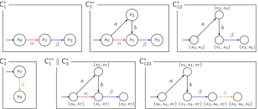
current element of that list. Finally, we return true. C∗1 s0 s1 s3 α _β C∗∗1 s0 s1 s2 s3 α a β b C∗12 (s0, s4) (s1, s4) (s2, s4) (s3, s6) a β b C∗3 s9 s7 δ C∗∗1 k C ∗ 3 (s0, s7) (s1, s7) (s2, s7) (s3, s7) α a β b C∗123 (s0, s4, s7) (s1, s4, s7) (s2, s4, s7) (s3, s6, s7) (s3, s6, s9) a β b δ

Figure 2 Some LTSs appearing during an execution of our algorithm on the example of Figure 1.

Back in the main function, Ls is consistent for now, so we move to the next iteration. Again both Ls[1] and Ls[2] are not complete because their current elements do not reach their objective. Let us say we concretise again Ls[1]. This time we cannot find an extension of ini(L1) k ini(L2) in the product of L1, L2and C∗1, which is empty. Then, since Left1is not

empty, we go to line 18, call Forget() (suppose here it forgets nothing), and set again the head of the list represented by Ls[1] (which is also the head of Left1) as the current element.

Then we return true again.

Back in the main function, Ls is still consistent and both its element are not complete. We then call Concretise() and for the example choose again k = 1. This time we extend C∗₁ by taking C∗∗₁ as the whole of L1 except the δ transition (Figure 2). Since Right1is not

empty this time, we go to line 7, update the tuples with C∗∗1 , and move the current element

of the list right, then return true.

Back in the main function we still call Concretise() and choose again k = 1. This time, we can extend ini(L1) k ini(L2) with the LTS C∗12 made only of the path (s0, s4), (s2, s4),

(s1, s4), (s3, s6) (Figure 2). Set N is empty because no LTS other than L1 and L2has labels β, a or b (used in this path). Right₁ is also empty so we just update the current element in Ls[1] with C∗₁₂(line 14) and return true.

Back in the main function, Ls[1] is now complete but not Ls[2]. So, we call Concretise() and choose k = 2. We extend ini(L3) by C∗3 made of the path s7, s9 (Figure 2). Then

N = {1} because L1 shares label δ with C∗3 and, as before, Right2 being empty, we go to

line 10, replace ini(L3) by C∗3, add the tuple (C ∗

3, ini(L3) k ini(L1), {3}, {3}, {1}) to the list

represented by Ls[2], and set that tuple as the current element of that list. Then we return true.

Now, we have the index 1 in J ∪ K for both the current elements of Ls[1] and Ls[2], so we can choose to merge them. Let us do it: we use the second of the simple strategies outlined

above: we keep and merge only the first and current elements of each list. After the call to Merge(), Ls = [([(id(L1) k id(L3), C∗∗1 k C

∗ 3, {1, 3}, ∅, {1, 3})], (C ∗∗ 1 k C ∗ 3, C ∗ 12 k ini(L3) k

ini(L1), {1, 3}, {1, 3}, {2}), [ ])] and C∗12k ini(L3) k ini(L1) consists only of state (s0, s4, s7),

because ini(L1) restricts C∗12 to its initial state and δ is not in C ∗

12. That product has no path

to a state (s3, ?, s9), so the new Ls[1] is not complete and we need to call Concretise() one

last time.

We will then be able to extend C∗₁₂k ini(L3) k ini(L1) to an LTS C∗123 containing state

(s3, s6, s9) but with no transition γ (Figure 2). Then N is empty, as well as Right1, so we go

through line 14 to update the current LTS, and return true. Finally, in the main function, we now have that Ls is consistent, since it contains only one element, and that element is complete because C∗₁₂₃contains only labels not shared with L4. So we terminate and return

true.

Note that we never needed to consider products involving L4 – which is the reason why

we call our analysis “lazy”.

3.4 Soundness, completeness, termination

We now proceed to proving that our algorithm is sound and complete and that it terminates. We first state two utility lemmas.

ILemma 16. Let (Left, h, Right) be an element of Ls in Solve(L, R) and let L = (ki∈[1..n]

Li).

Let (A, C, I, J, K) be either h, or an element of Left, or an element of Right. Then C is a partial product of (ki∈J ∪K Li) and, if we write C = (ki∈J ∪K Ci), then Σ(Ci) = Σ(Li).

ILemma 17. Let (Left, (A, C, I, J, K), Right) be an element of Ls in Solve(L, R). If Left

is empty then I ⊆ K, J = ∅ and A =ki∈Iid(Li).

And finally the main results:

IProposition 18. If Solve(L, R) returns False then R is not reachable in L.

Proof. The only way Solve(L, R) can return False is through line 12 in Algorithm 1, and in turn this means that the call to Concretise() in line 11 returned False. Now Concretise() will only return False through line 16 in Algorithm 2. To get there, there must exist some

k such that Ls[k] can be decomposed as the triple (Left, (A, C, I, J, K), Right), with (1) Left

being empty, and (2) there is no C∗s.t. C_{@ C}∗v (ki∈KLi) k A and C∗→ R|J∪K.

By Lemma 16 we know that C is a partial product of L. With (1) and Lemma 17, we have that I ⊆ K, J = ∅ and A =ki∈Iid(Li). So (ki∈KLi) k A = (ki∈KLi). Then, with (2),

we can deduce that R|K is not reachable in (ki∈KLi), and finally with the contrapositive of

Lemma 10, we get that R is not reachable in L. _J

IProposition 19. If Solve(L, R) returns True then R is reachable in L.

Proof. The only way Solve(L, R) can return True is through line 23 in Algorithm 1. This can only happen when Ls is such that (1) for all k, Ls[k] is complete and (2) Ls is consistent.

If we denote by (Ak, Ck, Ik, Jk, Kk) the second component of Ls[k], and by Hk the union

Jk ∪ Kk, (1) translates to ∀k, there exists C∗k v Ck such that C∗k can reach R|Hk and

{i 6∈ Hk : Σ(Li) ∩ λ(C∗k) 6= ∅} = ∅. Similarly, (2) translates to ∀i, j, Hi∩ Hj= ∅.

By Lemma 16, each C∗k is a partial product of (k i∈HkLi) (and thus also of L). Now

consider some i ∈ Hk and σ ∈ Σ(Li) ∩ λ(C∗k). By Lemma 16, we know that there exist

Σ(Li) ∩ λ(C) ⊆ Σ(Ci). From (2), we also have that ∀i 6∈ Hk, Σ(Li) ∩ λ(C) = ∅ and we

can thus use Lemma 11 and obtain that R|Hk is reachable in L, whatever the states of

the components not in Hk (and leaving them unchanged). Therefore, by finally putting all

components together, R is reachable in L. _J

Relation v is not sufficient to reflect progress in our algorithm. We therefore introduce a new relation <` , built on top of v, as a partial order over lists Ls (as the ones appearing

in Algorithm 1). Relation <` does reflect progress in concretisation (by advancing in the

history of concretisations (2), or by adding LTSs (3), or by adding paths in partial products (4,5)), and merging (by reducing the length of the list (1)).

IDefinition 20. Given two lists of tuples Ls1and Ls2with the same type as Ls in Algorithm 1,

we define <` such that Ls1<`Ls2 if and only if Ls16= Ls2 and:

len(Ls1) > len(Ls2), or (1)

len(Ls1) = len(Ls2) and ∀k, Ls1[k] 6= Ls2[k] =⇒ Ls1[k] <tLs2[k];

where (Left1, h1, Right1) <t(Left2, h2, Right2) if and only if, for hLri= rev(Lefti) ++[hi],

hLr2 is a prefix of rev(Left1), or (2)

∃`, hLr1[`] 6= hLr2[`] and, for the smallest such ` one has hLr1[`] <ahLr2[`];

where (A1, C1, I1, J1, K1) <a(A2, C2, I2, J2, K2) if and only if:

J1∪ K1⊂ J2∪ K2, or (3)

J1∪ K1= J2∪ K2 and A1@ A2, or (4) J1∪ K1= J2∪ K2, A1= A2, and C1@ C2. (5)

If Ls1<`Ls2or Ls1= Ls2we write Ls1≤`Ls2.

IProposition 21. The calls to Solve(L, R) always terminate (and return only True or

False).

Sketch of the proof. The fact that, if a call to Solve(L, R) terminates, it can only return True or False, comes from lines 23 (returning True) and 12 (returning False) of Algorithm 1 which are the only return statements of the Solve(, ) function.

In order to prove the termination one can show that (1) ≤` is an order relation over the

Ls used in Algorithm 1, (2) the set of such lists appearing in any instance of Algorithm 1 is finite (and so, there are lists which are greater or incomparable to any other lists with respect to ≤`), and (3) any step of the while loop of Algorithm 1 terminates and if the return of

line 12 is not used, strictly increases Ls with respect to ≤`. From (1) and (2) one then gets

that, in any instance of Algorithm 1, there cannot exist an infinite strictly increasing chain of Ls with respect to ≤`. Hence, from (3), Algorithm 1 always terminates. J

4

Experimental analysis

In order to get insight on the practical efficiency of our algorithm we developed a tool1

(LaRA, for Lazy Reachability Analyzer) using it. We then compared the time efficiency of LaRA with that of other tools on several reachability analysis tasks in distributed systems. We originally selected three other tools for these experiments:

LoLA2: A Petri net analyzer (it is straightforward to convert the compound systems we consider in this paper into (safe) Petri nets) which efficiently implements many techniques

1

For reproducibility of experiments, LaRA is available at http://lara.rts-software.org

2

for model checking Petri nets. LoLA is arguably very effective for reachability analysis in Petri nets as it won the reachability track at the last model checking contest [13]. PMC [14]: A tool for partial model checking that uses incremental techniques for dealing with the verification of distributed systems.

The on the fly model checking capabilities of the CADP toolbox [8]

Early preliminary experiments revealed that, on all our benchmarks, LoLA outperformed PMC and CADP. For the larger experiments on which we report here we thus focused on comparing LoLA with our tool.

4.1 Implementation choices

LaRA consists of approximately 500 lines of Haskell code, using the standard Parsec parsing library, and the fgl graph library. Note that memory management in Haskell is automatic.

We have presented our algorithm in a manner as generic as possible including the possibility for many heuristic choices. For our first prototype presented here, we have chosen to completely compute each partial product before adding more components. This eliminates the need for backtracking, which greatly simplifies the code and, to some extent, favors the case when the desired state is not reachable. This choice is rather drastic and probably not optimal when exploring big partial products, in which a more on-the-fly approach would usually give better results. However, we believe it is reasonable, as our objective was to evaluate the influence of the laziness feature of our approach.

Before adding LTSs to the partial product, we trim it by keeping only the reachable and coreachable states. We add only one automaton each time, chosen arbitrarily in the set of LTSs synchronized on the path that synchronizes as few LTSs as possible.

4.2 Benchmarks

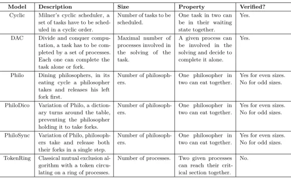
Our benchmarks where taken from a set of benchmarks proposed by Corbett in the 90’s [5]. Among these, we selected the ones where scaling increases the number of components but does not change the size of individual components. The reason for this choice is that our early implementation is not made for dealing with large state spaces of individual components – as, again, our goal is to evaluate the impact of its laziness feature. Not embedding efficient search techniques it was hopeless to cope with finely tuned model checking tools. This left us with six models, described in Table 1. For each model we define a simple reachability property and state if it is verified by the model.

Both tools were used in a similar setting: on a machine with four Intel® _Xeon® _E5-2620

processors (six cores each) with 128GB of memory. Though this machine has some potential for parallel computing, all the experiments presented here are actually monothreaded. We put a time limit of 20 minutes for computations. For each experiment, each tool had as input a file in its own format: file generation and conversion are not taken into account in the processing times.

4.3 Positive results.

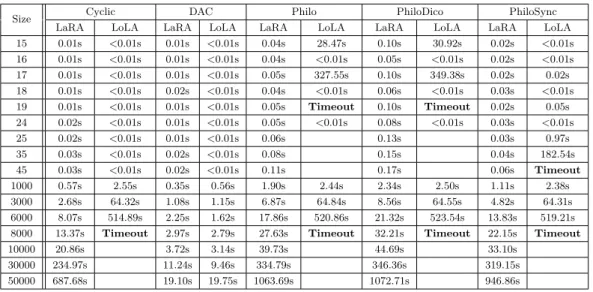
In most of the cases (namely Cyclic, Philo, PhiloDico, and PhiloSync) our tool outperformed LoLA with increasing size of models. On DAC, our results are comparable to those obtained with LoLA, and for very large instances we slightly outperform it. The experimental results for these cases are summarized in Table 2. For each model, timeout indicates the first

Table 1 Benchmarks description

Model Description Size Property Verified?

Cyclic Milner’s cyclic scheduler, a set of tasks have to be sched-uled in a cyclic order.

Number of tasks to be scheduled.

One task in two can be in their waiting state together.

Yes.

DAC Divide and conquer compu-tation, a task has to be com-pleted by a set of processes. Each one can complete the task alone or fork.

Maximal number of processes involved in the solving of the task.

A given process can be involved in the solving and decide to complete it alone.

Yes.

Philo Dining philosophers, in its eating cycle a philosopher takes and releases his left fork first.

Number of philosoph-ers.

One philosopher in two can eat together.

Yes for even sizes. No for odd sizes.

PhiloDico Variation of Philo, a diction-ary turns around the table, preventing the philosopher holding it to take forks.

Number of philosoph-ers.

One philosopher in two can eat together.

Yes for even sizes. No for odd sizes.

PhiloSync Variation of Philo, philosoph-ers take and release both their forks in a single step.

Number of philosoph-ers.

One philosopher in two can eat together.

Yes for even sizes. No for odd sizes. TokenRing Classical mutual exclusion

al-gorithm with a token circu-lating on a ring of processes.

Number of processes. Two given processes can reach their crit-ical section together.

No.

instance of this model for which a tool reached the time limit of 20 minutes. Notice that, in the variants of the dining philosophers, there are two timeouts: one for instances of odd size and the other one for instances of even size. This is because the property we verify is false for odd sizes and true for even sizes, which makes a significant difference for LoLA.

4.4 Focus on TokenRing.

Table 3 Runtimes on TokenRing.

Size TokenRing LaRA LoLA 7 0.514s <0.01s 8 1.716s <0.01s 9 6.713s <0.01s 10 25.810s <0.01s 11 70.370s <0.01s 12 322.440s <0.01s 13 Timeout <0.01s 1000 0.15s

Table 3 presents the results obtained with various modeling of TokenRing. It compares runtimes of LoLA and our tool on Corbett’s modeling. It appears that LaRA is far from efficient on this particular example. This is due to the fact that, without taking into account all the components, it is not possible for our tool to figure out that only one token exists in the system. So, for deciding that no two processes can be in their critical sections together, LaRA cannot be lazy and has to explore the full state space of the system.

5

Conclusion

We have presented a new approach for the verification of reachability in distributed systems. It builds on both decomposing the goal state into its projection on the different components of the system and lazily adding components in an iterative fashion to produce more and more precise over-approximations. This notably allows for early termination both when the state is reachable and when it is not. We have presented an algorithm based on this approach, together with proofs for completeness, soundness, and termination. We have also

Table 2 Comparison of runtimes of LoLA and LaRA on instances of increasing size of Cyclic,

DAC, Philo, PhiloDico, and PhiloSync.

Size Cyclic DAC Philo PhiloDico PhiloSync

LaRA LoLA LaRA LoLA LaRA LoLA LaRA LoLA LaRA LoLA 15 0.01s <0.01s 0.01s <0.01s 0.04s 28.47s 0.10s 30.92s 0.02s <0.01s 16 0.01s <0.01s 0.01s <0.01s 0.04s <0.01s 0.05s <0.01s 0.02s <0.01s 17 0.01s <0.01s 0.01s <0.01s 0.05s 327.55s 0.10s 349.38s 0.02s 0.02s 18 0.01s <0.01s 0.02s <0.01s 0.04s <0.01s 0.06s <0.01s 0.03s <0.01s 19 0.01s <0.01s 0.01s <0.01s 0.05s Timeout 0.10s Timeout 0.02s 0.05s 24 0.02s <0.01s 0.01s <0.01s 0.05s <0.01s 0.08s <0.01s 0.03s <0.01s 25 0.02s <0.01s 0.01s <0.01s 0.06s 0.13s 0.03s 0.97s 35 0.03s <0.01s 0.02s <0.01s 0.08s 0.15s 0.04s 182.54s 45 0.03s <0.01s 0.02s <0.01s 0.11s 0.17s 0.06s Timeout 1000 0.57s 2.55s 0.35s 0.56s 1.90s 2.44s 2.34s 2.50s 1.11s 2.38s 3000 2.68s 64.32s 1.08s 1.15s 6.87s 64.84s 8.56s 64.55s 4.82s 64.31s 6000 8.07s 514.89s 2.25s 1.62s 17.86s 520.86s 21.32s 523.54s 13.83s 519.21s 8000 13.37s Timeout 2.97s 2.79s 27.63s Timeout 32.21s Timeout 22.15s Timeout

10000 20.86s 3.72s 3.14s 39.73s 44.69s 33.10s

30000 234.97s 11.24s 9.46s 334.79s 346.36s 319.15s 50000 687.68s 19.10s 19.75s 1063.69s 1072.71s 946.86s

implemented this into an early prototype named LaRA. This rather naive implementation already gives very promising results, on which we report together with comparisons to LoLA, a state-of-art model-checker for Petri nets.

Further note that, when a reachability property is true, LaRA has computed, and can output, a consistent list of complete LTSs satisfying that property. An interesting plus-value is that adding whatever number of new components to that list would not change the outcome provided that none of those new components shares actions that are used in the list. Therefore in systems with a particular synchronization structure, like rings for instance, we can generalize the reachability result to any number of components in the ring : for instance to prove that a philosopher can eat we need to add the two forks around her and the other two philosophers that could also use those forks. Now, any additional fork or philosopher beyond those do not share any action required to establish that the first philosopher can eat. We can then deduce that she can eat regardless of the number of philosophers around the table.

We have proposed and proved our algorithm in a generic and extendable way. In particular, it seems very likely that partial order or Decision Diagram-based symbolic techniques could be incorporated in this approach. The algorithm we propose also offers several opportunities for parallelisation. First, between two merge operations all concretisations in the different partitions can clearly be performed in parallel. Second, the different choices left open in the algorithm, such as the choice of a particular path to concretise, or a specific automaton to add to the product, can be resolved by some heuristics but may also better be handled by testing several of the different choices in parallel.

In addition to studying theses issues, further work includes extensions to more expressive formalisms, in particular (parametric) timed automata and time Petri nets, and to more complex properties.

Acknowledgments. We gratefully thank Frédéric Lang for the time he spent helping us

to use his partial model checking tool. We also thank Karsten Wolf for offering help with LoLA. Finally, we thank the anonymous reviewers for their valuable comments.

References

1 H. R. Andersen. Partial model checking. In LICS, pages 398–407, 1995.

2 F. Bacchus and Q. Yang. Downward refinement and the efficiency of hierarchical problem solving. Artificial Intelligence, 71(1):43–100, 1994.

3 A. R. Bradley. SAT-based model checking without unrolling. In VMCAI, pages 70–87, 2011.

4 A. Cimatti and A. Griggio. Software model checking via IC3. In CAV, pages 277–293, 2011.

5 J. C. Corbett. Evaluating deadlock detection methods for concurrent software. IEEE Trans.

Software Eng., 22(3):161–180, 1996.

6 P. Crouzen and F. Lang. Smart reduction. In FASE, pages 111–126, 2011.

7 C. Flanagan and S. Qadeer. Thread-modular model checking. In SPIN, pages 213–224, 2003.

8 H. Garavel, F. Lang, R. Mateescu, and W. Serwe. CADP 2011: a toolbox for the construc-tion and analysis of distributed processes. STTT, 15(2):89–107, 2013.

9 S. Graf and B. Steffen. Compositional minimization of finite state systems. In CAV, pages 186–196, 1990.

10 O. Grumberg and D. E. Long. Model checking and modular verification. TOPLAS,

16(3):843–871, 1994.

11 J. Hoffmann, J. Porteous, and L. Sebastia. Ordered landmarks in planning. JAIR,

22(1):215–278, 2004.

12 G. J. Holzmann and D. Peled. An improvement in formal verification. In FORTE, pages 197–211, 1994.

13 F. Kordon, H. Garavel, L. M. Hillah, F. Hulin-Hubard, A. Linard, M. Beccuti, A. Hamez, E. Lopez-Bobeda, L. Jezequel, J. Meijer, E. Paviot-Adet, C. Rodriguez, C. Rohr, J. Srba, Y. Thierry-Mieg, and K. Wolf. Complete Results for the 2015 Edition of the Model Checking Contest. http://mcc.lip6.fr/2015/results.php, 2015.

14 F. Lang and R. Mateescu. Partial model checking using networks of labelled transition systems and boolean equation systems. LMCS, 9(4), 2013.

15 A. Lehmann, N. Lohmann, and K. Wolf. Stubborn sets for simple linear time properties. In ICATPN, pages 228–247, 2012.