Science Arts & Métiers (SAM)
is an open access repository that collects the work of Arts et Métiers Institute of Technology researchers and makes it freely available over the web where possible.
This is an author-deposited version published in: https://sam.ensam.eu
Handle ID: .http://hdl.handle.net/10985/17327
To cite this version :
Gnofam Jacques TCHEIN, Dimitri JACQUIN, Egoitz ALDANONDO, Dominique COUPARD, Esther GUTIERREZ-ORRANTIA, Franck GIROT MATA, Eric LACOSTE - Analytical modeling of hot behavior of Ti-6Al-4V alloy at large strain - Materials & Design - Vol. 161, p.114-123 - 2019
Any correspondence concerning this service should be sent to the repository Administrator : archiveouverte@ensam.eu
Analytical modeling of hot behavior of Ti-6Al-4V alloy at large strain
Gnofam Jacques TCHEIN a,b, Dimitri JACQUIN a, Egoitz ALDANONDO c, Dominique
COUPARD d, Esther GUTIERREZ-ORRANTIA b, Franck GIROT MATA b, Eric LACOSTE a
a
Univ. Bordeaux, I2M, UMR 5295, CNRS, F-33400 Talence, France
b
University of the Basque Country, UPV/EHU, Faculty of Engineering, Department of Mechanical
Engineering, Alameda de Urquijo s/n, Bilbao, Bizkaia, Spain
c Lortek, Arranomendia kalea 4A, 20240 Ordizia (Gipuzkoa), Spain
d Arts et Métiers ParisTech, I2M, UMR 5295, CNRS, Esplanade Arts et Métiers, F-33400 Talence,
France
Corresponding author: Dimitri JACQUIN
I2M, UMR 5295, Site IUT - 15, rue Naudet - CS 10207 - 33175 - Gradignan Cedex – France Tel.: (33)5 56 84 58 65 – Fax: (33)5 56 84 58 43 – email: dimitri.jacquin@u-bordeaux.fr
ABSTRACT
Hot deformation behavior of the Ti-6Al-4V alloy is studied through hot torsion tests. Cylindrical samples are twisted at different strain rates and temperatures in the β phase domain. The recorded torque vs twisting angle data are converted to strain vs stress data using the appropriate methods. All the flow curves obtained are characteristic of continuous dynamic recrystallization. The flow stresses exhibit rapid growth to reach a single maximum followed by a decrease and a steady-state regime. The influence of strain rate and temperature is taken into account. An analytical model is proposed, which gives accurate flow curves for the Ti-6Al-4V alloy for processing temperatures between
1000°C and 1100°C and strain rates between 0.01/s and 1/s. The model is validated by further experimental tests.
Keywords:
Large strain - Hot behavior - Ti-6Al-4V alloy - Flow stress - Analytical behavior law - Torsion test
1. Introduction
Titanium alloys have been used for many years due to their good mechanical properties, such as corrosion resistance and low density. The Ti-6Al-4V alloy in particular, which retains its good mechanical properties at high temperature, is widely used in the aerospace industry.
Titanium and its alloys have two allotropic forms. At low temperatures, pure titanium has a hexagonal closed packed (HCP) structure, which is commonly known as α, whereas above 883°C, it has a body centered cubic (BCC) crystal structure termed β. The alloying elements can increase or decrease the β transus temperature. α+β alloys have both phases below the β transus temperature and only the β phase above. For the Ti-6Al-4V alloy especially, the β transus temperature is
approximately 995°C. Depending on whether the operating temperature is below or above the β transus, the material should have a different flow behavior and thus different rheological parameters [1]. The study of its behavior at high temperatures is essential when we need to model hot processes such as Friction Stir Welding.
The hot rheological properties of titanium alloys can be studied using hot compression [2] or hot torsion tests. Hot compression tests are suitable for determining material behavior at low strains [3]. They are usually performed at temperature ranges higher than half the melting temperature value: the minimum processing temperature reported to provide recrystallized microstructure in metallic materials [4]. Hot compression tests in the dual phase domain usually exhibit different results from tests in the β phase domain [5]. Mechanisms of deformation of Ti-6Al-4V in the β phase domain were investigated by [6] through hot compression. A steady state was observed for all flow
curves performed at strain rates less than or equal to 1/s. Above this value, the flow stress oscillated and did not reach a steady value. Prasad et al. [6] used an Arrhenius type equation to model the steady-state flow stress ; the prior β grain size was also modeled as a function of the Zener-Hollomon parameter using a power law. Ning et al. [7] compressed the TC18 at temperatures between 800 and 900°C and strain rates from 0.01/s and 1/s. The activation energy and the strain rate sensitivity were calculated and their evolution as a function of strain rate and temperature were examined.
Compression of TC11 alloy in temperature ranges from 750 to 950°C [8] produced dynamically recrystallized α grains. Optimal processing conditions which could provide a good refined microstructure with low stress were estimated at 950°C and 0.001/s.
Large deformation studies on metals can be achieved via hot torsion or Severe Plastic Deformation (SPD) tests [9]. With hot torsion it is possible to apply large deformations while keeping the sample length constant. This test is well adapted to represent phenomena occurring during FSW manufacturing [10], for example, where very large strains are reached (equivalent strain more than 20) [11]. Hot torsion tests are likely to provide similar microstructures to that of friction stir processing [12], while SPD is known to induce microstructure refinement [13]. During hot torsion of Ti-6Al-4V, different deformation modes were observed according to the allotropic form: dynamic recrystallization for the α+β phase domain and dynamic recovery for the β phase domain [14]. Continuous dynamic recrystallization is reported to be the main phenomenon governing the microstructure after large deformation during hot torsion of the titanium alloy Ti17 above the β transus temperature [15].
The aim of this work is to provide a fast and accurate behavior law for Ti-6Al-4V titanium alloy, useful for all work requiring knowledge of the behavior of the alloy within the range of strain rate between 𝜀̅̇ = 0.01𝑠−1 and 𝜀̅̇ = 1𝑠−1, the range of strain between 𝜀̅ = 0 and 𝜀̅ = 15 and a range of temperature between 1000°C and 1100°C. This work is part of an approach to simplify access to these types of behavior laws which often require very expensive material characterization equipment not always available in the laboratory. The behavior laws are necessary to carry out many
simulations. For instance, when using a finite element software such as Abaqus, Forge Zset, .etc., the researcher usually implements the behavior law point by point, to fit the hot behavior of the material as well as possible during loading. This tedious step often involves simplifying assumptions and this can sometimes lead to significant discrepancies from reality. In addition, as many tests as loading conditions must be reproduced, and since the range of tests is often discrete, it does not cover the entire range of the digital tests. The researcher is therefore forced to use digital interpolation techniques, and therefore produces threshold results.
This work proposes to remove the problem by proposing a fully integrated analytical and continuous behavior law which can be used to simulate manufacturing processes such as FSW or SPD, wire-drawing or stamping [16]. A full description and instructions for use of this law are provided at the end of this paper.
2. Experimental procedures 2.1. Test machine and samples
The machine is composed of a motor, a gear box, a clutch, a torque measurement system and two shafts. The first shaft is fixed, while the second one is used to apply the torque. The machine is software controlled and records three data at a frequency of one hundred per second: the current time, the couple and the number of revolutions. The machine test has an infrared heating system which heats the sample up to the testing temperature. An argon gas flow is used as shielding gas to prevent oxidation.
The tubular torsion samples consisted of a calibrated part and two threaded shoulders. The calibrated part was 18 mm long and had a diameter of 7.5 mm (Erreur ! Source du renvoi introuvable. 1). A hole was drilled on the side of the sample to insert the thermocouple used to control the temperature.
Fig. 1 Experimental sample before deformation (A) and after deformation at 1050°C and 0.5/s (B)
At the end of the process, the sample is quickly removed from the oven and water quenched to room temperature.
2.2. Data processing
The data processing consists of converting the number of revolutions N vs torque data to strain vs stress data. With the hot torsion test, the evolution of function of N for a given
temperature and strain rate can be obtained. Equivalent strain is calculated using a method proposed by Montheillet and Desrayaud [17].
By assuming that the sample is perfectly homogenous, one can show that the rotational speed 𝜔̇(𝑧)varies linearly from the fixed side to the rotating side of the sample (Fig. 2).
Fig. 2 Schematic representation of a test sample
As the radius and the length of the sample are assumed to remain constant, their
corresponding velocity fields are null. The velocity field is expressed in the cylindrical coordinates system as follows: { 𝒗𝒓 = 𝟎 𝒗𝜽 =𝑳𝒛𝒓𝛀̇ 𝒗𝒛 = 𝟎 (2)
Then the velocity gradient tensor in cylindrical coordinates and the strain rate tensor are expressed respectively as Eq. (3) and Eq. (4):
𝒈𝒓𝒂𝒅 𝒗 = [𝟎 −𝒛 𝟎𝒛 𝟎 𝒓 𝟎 𝟎 𝟎 ]𝛀̇𝑳 (3) 𝜺̇ = [𝟎 𝟎 𝟎𝟎 𝟎 𝒓 𝟎 𝒓 𝟎 ]𝟐𝑳𝛀̇ (4)
The equivalent von Mises strain rate and the equivalent strain are expressed as follows Eq. (5) and Eq. (6):
𝜺̅̇ = 𝛀̇𝒓 √𝟑𝑳=
𝟐𝝅𝑵̇𝒓
√𝟑𝑳 (5)
𝜺̅ =√𝟑𝑳𝛀𝒓 =𝟐𝝅𝑵𝒓√𝟑𝑳 (6)
It can be observed that the strain at a position in the sample is only a function of the radial position. The strain in the axis is null and maximum at the outer surface of the sample.
The flow stress at the surface of the cylindrical specimen is calculated using the method proposed by Fields and Backofen [18]. They demonstrated that equivalent flow stress in the surface of the sample as a function of the torque is Eq. (7):
𝜎̅ =2𝜋𝑅√3Γ3(3 + 𝑛̃ + 𝑚̃) (7)
where R is the radius of the specimen. 𝑛̃ and 𝑚̃, which denote the sensitivity of the couple to strain and to strain rate respectively, are functions of processing parameters and N. They are calculated through the following equations Eq. (8) and Eq. (9):
𝒏̃ =𝝏𝒍𝒏𝑵𝝏𝒍𝒏𝜞|
𝑵̇,𝑻 (8)
𝒎̃ =𝝏𝒍𝒏𝑵̇𝝏𝒍𝒏𝜞|
𝑵,𝑻 (9)
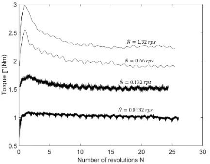
The flow curves give N vs (Fig. 3). The ln (Γ) is correlated to ln (N) through a third degree
polynomial function (Fig. 4). Sensitivity to strain 𝑛̃ is then retrieved by deriving the polynomial function.
Fig. 3 𝚪 𝒗𝒔 𝑵 data for tests performed at 1000°C and different revolutions per second (rps)
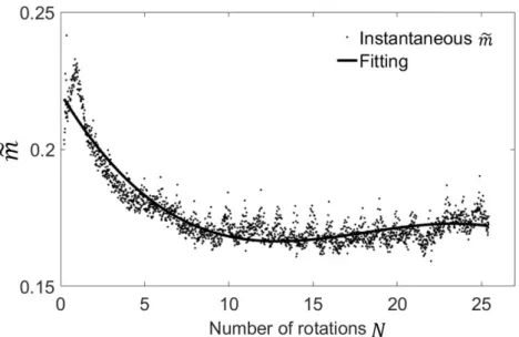
Fig. 4 𝐥𝐧 (𝚪) vs 𝐥𝐧 (𝐍) data for tests at T=1000°C and different revolutions per second (rps) The strain rate sensitivity m̃ is calculated for each value of N. It is given by the slope of the ln(Γ) vs ln (Ṅ) data. Finally, the strain rate sensitivity values are related to N through a third degree polynomial (Fig. 5).
Fig. 5 𝒎̃ values obtained for T=1000°C
From the results obtained previously, it is possible to follow the evolution of the equivalent flow stress, the equivalent strain rate and the equivalent strain from Eq. (4), (5) and (6).
3. Results and discussion 3.1. Strain-stress curves
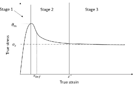
The experiments were performed at three different temperatures from 1000°C to 1100°C and strain rates from 0.01/s to 1/s, as shown in Table 1. The flow curves obtained from the tests can be divided into three stages and confirm a previous study in which it was shown that titanium could undergo Continuous Dynamic Recrystallisation during friction stir welding [19] (Fig. 6).
During the first stage, the dislocations multiply and interact, leading to an increase in stress. The stress grows rapidly and reaches its maximum value. The second stage consists of a softening. This stage begins when dynamic recovery becomes greater than hardening. In this stage, the stress decreases slowly from its maximum to its steady-state, passing through an inflection point. The last stage is the stationary domain where the flow stress value remains constant. The recovery and strain hardening phenomena are balanced and the final microstructure reaches an equilibrium state.
These results are different from those of low stacking fault energy materials which undergo Discontinuous Dynamic Recrystallization (DDRX), where a series of oscillations with decreasing amplitude are usually observed [20]. The strain corresponding to the inflection point is named 𝜀𝑖𝑛𝑓.
The experimental curves can then be compared by using four parameters: the maximum stress value 𝜎𝑚, the critical strain 𝜀∗ for stationary stress, the value of the steady state flow stress 𝝈̅
𝑆 and the strain on the inflection point 𝜀𝑖𝑛𝑓 (Table 1).
Fig. 6 Schematic representation of a typical flow curve
Table 1 Experimental table
Test no. Temperature (°C) Strain rate (1/s) Maximum stress 𝜎̅𝑚 (MPa) Critical
strain 𝜀∗ Steady-state stress 𝜎̅ 𝑆 (MPa) 𝜀𝑖𝑛𝑓 1 1000 0.01 18.37 4 16.26 5.5 2 1000 0.1 28.39 6 24.83 3.7 3 1000 0.5 41.99 6 31.17 2.97 4 1000 1 49.27 9 37.45 2.67 5 1050 0.01 13.65 4 12.28 5.5 6 1050 0.1 24.26 6 20.69 3.7 7 1050 0.5 37.38 8 29.55 2.97 8 1050 1 44.04 9 33.48 2.67 9 1100 0.01 13.30 4 10.47 5.5 10 1100 0.1 21.72 6 17.13 3.7 11 1100 0.5 38.08 7 24.99 2.97 12 1100 1 42.75 9 31.52 2.67
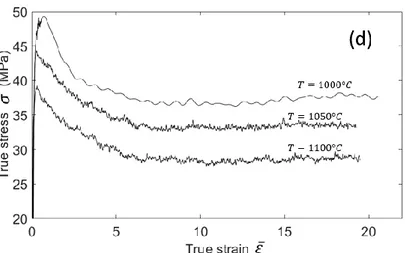
The curves obtained under the conditions mentioned in Table 1 are represented in Fig. 7 and Fig. 8.
Fig. 8 Flow curves obtained at 0.01/s (a), 0.1/s (b), 0.5/s (c) and 1/s (d) for different temperatures
From Fig. 7 and Fig. 8, we observe that the flow curves’ characteristics, namely 𝝈̅𝑆, 𝝈̅𝑚 , 𝜀𝑖𝑛𝑓 and 𝜀∗, depend on temperature and strain rate. The steady-state flow stress and the maximum stress increase by increasing the strain rate and decrease by increasing the temperature. The effect of strain rate on the flow stress can be related to metallurgical aspects involved in this process. The maximum stress increases sharply for high strain rates and more gently for lower strain rates.
The critical strain 𝜀∗ and 𝜀
𝑖𝑛𝑓 were read from the flow curve plots. Both parameters are strongly dependent on strain rate, especially 𝜀𝑖𝑛𝑓 which is independent of temperature. They evolve in the same way as the strain rate.
3.2. Rheological parameters
During hot forming processes, the steady-state flow stress and the thermomechanical
parameters are usually related through empirical behavior laws. These laws allow the determination of rheological parameters that characterize temperature and strain rate sensitivity of a material. An example is the Zener-Hollomon relationship given in Eq.𝝈=𝑲𝜺̅̇𝒎𝐞𝐱𝐩 (𝒎𝑸
𝑹𝑻) which relates equivalent stress to equivalent strain in the steady-state domain.
𝝈
̅ = 𝑲𝜺̅̇𝒎𝐞𝐱𝐩 (𝒎𝑸
where 𝐾 is a constant, 𝑚 is the strain rate sensitivity, 𝑄 is the apparent activation energy and 𝑅 is the gas constant. The apparent activation energy describes the activation barrier that atoms need to conquer to follow the deformation procedure. The strain rate sensitivity characterizes the effect of the strain rate on the flow stress. In the case of titanium alloys, it is generally admitted that strain-rate sensitivity depends on the allotropic phase [1]. These parameters can be determined at a given deformation by using Eq.𝝈=𝑲𝜺̅̇𝒎𝐞𝐱𝐩 (𝒎𝑸
𝑹𝑻) and Eq. (12).
𝒎 =
𝝏𝒍𝒏 (𝝈𝝏𝒍𝒏 (𝜺̅̇)̅)|
𝑻,𝜺̅ (11)
𝑸 =
𝝏𝒍𝒏 (𝝈𝝏(𝟏/𝑻)̅)|
𝜺̅̇,𝜺̅ (12)
The Eq. (10) and (11) show that 𝑚 and 𝑄 depend on temperature and strain rate respectively. It is usual to choose their respective mean values. Another way to calculate them independently of temperature and deformation rate is to rely on Eq. (9) by calculating the logarithm of the 2 equality members, Eq. (13).
𝐥𝐧(𝝈̅) = 𝐥𝐧(𝑲) + 𝒎 𝐥𝐧(𝜺̅̇) +𝒎𝑸𝑹 𝑻𝟏 (13)
ln(𝐾) , 𝑚 and 𝑚𝑄𝑅 are determined by a linear fitting of ln(𝜎̅) as a function of ln(𝜀̅̇) and 𝑇1 . The values obtained for 𝑚 and 𝑄 are respectively 0.21 and 270 𝑘𝐽/𝑚𝑜𝑙. Similar values of activation energy and strain rate sensitivity were found by other investigations [21] during hot working of Ti-6Al-4V in the β phase domain.
While the rheological parameters give information about the temperature and strain rate sensitivity of the material in the steady state regimes, they are not able to describe the complete material behavior at a given temperature and strain rate, at transient regimes.
4. Analytical modeling of flow curves 4.1. Modeling
In this section, an analytical model is proposed to fit the flow curve profiles as a function of temperature and strain rate. The aim of this model is to plot stress as a function of strain for the processing conditions included in our study range. It has some advantages compared to other models because it takes into account both strain hardening and dynamic recovery. In contrast, other models like those of Sellars and Tegart [22] do not take strain hardening into account. The Johnson-Cook model [23] considers strain hardening but does not consider dynamic recrystallization. A 2D model developed by Calamaz et al. [24] for chip formation when machining Ti-6Al-4V alloy takes dynamic recrystallization into account, but is limited to lower temperatures and strains. In such temperature ranges, other parameters like grain size should be taken into account as Velay et al. [25] did but for very low strain rate ranges.
The proposed model gives an accurate evolution of stress as a function of strain for hot working of Ti-6Al-4V. The constitutive laws are given to determine the parameters as a function of strain rate and temperature within our processing conditions i.e. for strain rates within 0.01/s – 1/s and temperatures within 1000°C – 1100°C. For this range of temperatures, a previous investigation showed that the initial grain size does not affect the final microstructure [19]. In future
investigations, a broader range of processing conditions will be covered.
The proposed mathematical formulation of the function F, which represents the stress
evolution function of strain rate, is based on an exponential function coupled with a tanh function in order to model the strain softening effect:
𝝈
̅ = 𝑭 = 𝒎𝟏𝜺̅𝒂(𝟏 + 𝜺̅)−𝒂(𝟏 − 𝒎𝟐𝐭𝐚𝐧𝐡 (𝜺̅ 𝜺⁄ 𝒊𝒏𝒇)) (14) where 𝑚1, 𝑚2, and 𝑎 are coefficients which depend on thermomechanical parameters.
The function F can be subdivided into three terms F1, F2 and F3, expressions of which are given in Eq. (15): { 𝑭𝟏= 𝒎𝟏𝜺̅𝒂 𝑭𝟐= (𝟏 + 𝜺̅)−𝒂 𝑭𝟑= 𝟏 − 𝒎𝟐𝐭𝐚𝐧𝐡 (𝜺̅ 𝜺⁄ 𝒊𝒏𝒇) (15)
An example based on the flow curve obtained at 1100°C and 0.1/s, of the graphical representation of the functions F1, F2 and F3 is given in Fig. 9. For very low strains, 𝐹2 and 𝐹3 are close to 1, so 𝐹 ≈ 𝐹1. For such strains, the stress evolution is then modeled with a power law function. For medium and high strains, the drop in stress as a result of dynamic recovery is outlined by 𝐹3 while 𝐹2 annihilates the increase in the hardening term 𝐹1. Finally, for very high strains, 𝐹 reaches a stationary value 𝐹𝑠𝑡𝑎 which is independent of strain and represents the steady state flow stress Eq. (16):
𝑭𝒔𝒕𝒂 ≈ 𝒎𝟏 (𝟏 − 𝒎𝟐) (16)
Fig. 9 Flow curve of test performed at 1050°C and 0.5/s and plot of the representative functions F1, F2 and F3
The fitting of each flow curve requires the determination of the adequate set of parameters (𝑚1, 𝑚2, 𝑎, 𝜀𝑖𝑛𝑓).
4.2. Identification of parameters
The model parameters have been identified to fit the flow curves of the current experiments. This minimization problem was solved using the Matlab® R2016a [26] fmincon function. fmincon resolves optimization problems by determining the minimum of a constrained linear or nonlinear multivariable function. The input values of the solver are the function to be minimized, the constraints, the initial solution and the algorithm to be used.
The function to be minimized is the residual 𝜹 between the predicted stress and the experimental data expressed in relation Eq. (17).
{
𝛿 = ∑ (𝜎𝑖 𝑖− 𝐹𝑖)2 𝐹𝑖 = 𝑚1𝜀̅𝑖𝑎(1 + 𝜀̅
𝑖)−𝑎(𝟏 − 𝒎𝟐𝒕𝒂𝒏𝒉 (𝜺̅𝒊⁄𝜺𝒊𝒏𝒇)) (17)
𝜎𝑖 and 𝐹𝑖 represent respectively the experimental stress and the corresponding predicted stress for the experiment i. The function 𝐹𝑖 was constrained to pass through the maximum of the experiment flow curve. Eq. (18) is therefore used as equality constraint for each experiment.
𝒎𝟏𝜺̅𝒎𝒂(𝟏 + 𝜺̅𝒎)−𝒂(𝟏 − 𝒎𝟐𝒕𝒂𝒏𝒉 (𝜺̅𝒎⁄𝜺𝒊𝒏𝒇)) = 𝝈̅𝒎 (18)
Where 𝜀̅𝑚 is the experimental strain corresponding to the maximum stress.
Two algorithms are available for fmincon, namely the SQP method (Sequential Quadratic Programming) and the Interior Point method. Both methods have advantages and disadvantages. The main differences between them were outlined here [27]. After many trials, the SQP method was identified as the most suitable method that could solve our problem efficiently. The initial solution that best fits the flow curve was determined by numerical means. First, an adequate interval for each parameter was identified. Second, combinations of different variables were made in their respective intervals and the set of parameters that minimizes the residual was used as an initial solution.
The different sets of parameters m1, m2 and a, for the 12 experiments obtained through the
fmincon solver are summarized in Table 2. These coefficients need to be correlated to processing
conditions to complete the model.
Table 2 Parameters of the model
Test n° 𝑚1 (MPa) 𝑚2 𝑎 1 20.79 0.19381631 0.13527816 2 30.06 0.18327317 0.02968457 3 54.12 0.40588561 0.2 4 72.30 0.46793499 0.28825596 5 15.60 0.20944449 0.14834964 6 27.29 0.24 0.08794759 7 41.34 0.30663119 0.09 8 53.34 0.37047608 0.10085617 9 16.07 0.32513471 0.19196688 10 27.67 0.37425915 0.19867846 11 47.87 0.44903248 0.21 12 53.03 0.38730959 0.11946056
4.3. Correlation of model parameters to thermomechanical conditions
The model coefficients are related to strain rate and temperature so that the correlation of 𝑚1 and 𝑚2 is performed through multilinear polynomials while 𝜀𝑖𝑛𝑓, which depends solely on strain rate, is modeled with a power la, Eq. (19). The power exponent 𝑎 was found to be dependent on the three parameters 𝑚1, 𝑚2 and 𝜀𝑖𝑛𝑓. Next, a multilinear polynomial was used to describe its evolution. The method used here to determine coefficients is the least squares method.
(19) where 𝑥 = 𝑙𝑛(𝜀̅̇) and 𝑦 = 𝑇 where T is expressed in Kelvin.
The model coefficients obtained are summarized in Table 3.
{ 𝑚1= 𝑝0,𝑚1+ 𝑝1,𝑚1𝑥 + 𝑝2,𝑚1𝑦 + 𝑝3,𝑚1𝑥𝑦 + 𝑝4,𝑚1𝑥2+ 𝑝 5,𝑚1𝑦 2+ 𝑝 6,𝑚1𝑥 2𝑦 + 𝑝 7,𝑚1𝑥𝑦 2 𝑚2= 𝑝0,𝑚2+ 𝑝1,𝑚2𝑥 + 𝑝2,𝑚2𝑦 + 𝑝3,𝑚2𝑥𝑦 + 𝑝4,𝑚2𝑥2+ 𝑝5,𝑚2𝑦2+ 𝑝6,𝑚2𝑥2𝑦 + 𝑝7,𝑚2𝑥𝑦2 𝑎 = 𝑝0,𝑎+ 𝑝1,𝑎𝑚1+ 𝑝2,𝑎𝑚2+ 𝑝3,𝑎𝜀𝑖𝑛𝑓+ 𝑝4,𝑎𝑚1𝑚2+ 𝑝5,𝑎𝑚2𝜀𝑖𝑛𝑓+ 𝑝6,𝑎𝑚1𝜀𝑖𝑛𝑓 𝜀𝑖𝑛𝑓 = 𝑝0,𝜀𝑖𝑛𝑓𝜀̅̇𝑝1,𝜀𝑖𝑛𝑓
Table 3 Model coefficients for processing temperatures between 1000°C and 1100°C and strain rates between 0.01/s and 1/s 𝒑𝟎,𝒎𝟏 𝒑𝟏,𝒎𝟏 𝒑𝟐,𝒎𝟏 𝒑𝟑,𝒎𝟏 𝒑𝟒,𝒎𝟏 𝒑𝟓,𝒎𝟏 𝒑𝟔,𝒎𝟏 𝒑𝟕,𝒎𝟏 6347.4949 1267.91481 -9.35305727 -1.78232168 26.3216568 0.00347361 -0.01847277 0.00063231 𝒑𝟎,𝒎𝟐 𝒑𝟏,𝒎𝟐 𝒑𝟐,𝒎𝟐 𝒑𝟑,𝒎𝟐 𝒑𝟒,𝒎𝟐 𝒑𝟓,𝒎𝟐 𝒑𝟔,𝒎𝟐 𝒑𝟕,𝒎𝟐 58.193006 6.905186 -0.08686 -0.008903 0.298427 0.000033 -0.00022 0.000003 𝒑𝟎,𝒂 𝒑𝟏,𝒂 𝒑𝟐,𝒂 𝒑𝟑,𝒂 𝒑𝟒,𝒂 𝒑𝟓,𝒂 𝒑𝟔,𝒂 - -0.092043 -0.005727 0.019137 0.012073 0.010605 0.082919 0.001328 - 𝒑𝟎,𝜺𝒊𝒏𝒇 𝒑𝟏,𝜺𝒊𝒏𝒇 - - - - 2.636 -0.1585 - - - -
From Eq. Erreur ! Source du renvoi introuvable.) and Table (3), coefficients 𝑚1,
𝑚2 𝑎 and 𝜀𝑖𝑛𝑓 are calculated. The model is then compared to the experimental flow curves (Fig. 10): we can observe good agreement between experimental and model results. The tolerance of the model is estimated at ±3 MPa.
Fig. 10 Model vs experimental flow curves for tests at 1000°C (a), 1050°C (b) and 1100°C (c)
4.4. Validation
The proposed algorithm (Fig. 11) provides the complete stress-strain curves for hot deformations of Ti-6Al-4V alloy within the experimental conditions range i.e. strain rates and temperatures between 0.01 – 1/s and 1000 – 1100°C respectively.
Fig. 11 Proposed algorithm for determining flow curves
In order to validate the algorithm, three other processing conditions (1050°C – 0.05/s, 1050°C – 0.25/s and 1050°C – 0.75/s) have been performed. Corresponding flow curves are presented in Fig. 12. These curves are compared with calculated curves obtained from previous model (Fig. 12). This figure shows a very good agreement between the model and the experimental results.
Fig. 12 Comparison between model and validation tests performed at 1050°C and different strain rates
5. Conclusion
In this study, a complete and accurate continuous analytical constitutive law is proposed to model the hot behavior of the widely used Ti-6Al-4V alloy within the equivalent strain rate 0.01 and 1/s and a temperature range between 1000 and 1100°C.
This model can provide the analytical constitutive law for large deformation and transient regimes. Thus, this analytical behavior law intrinsically takes into account the metallurgical effects of the hot strain of the Ti-6Al-4V: continuous dynamic recrystallization, phase transformation, given that it is fully based on experimental investigations.
This analytical constitutive law can be freely reused by those needing to know the hot behavior of Ti-6Al-4V. For instance, this work will be very useful for different processing such as forging, stamping, rolling mills, wire drawing or friction stir welding, where large hot deformations occur.
This work opens the way to a fully analytical model which will lead to a drastically reduced computation time. It makes it possible to provide a behavior law continuously over the entire field of application, thus avoiding the need for usual digital interpolation techniques.
Finally, this analytical modeling could be associated with microstructural modeling, to enhance the accuracy of the flow stress computation.
ACKNOWLEDGMENTS
This work was supported by IdEx Bordeaux within the framework of the Cross-border Joint Laboratory ‘‘Aquitania Euskadi Network In Green Manufacturing and Ecodesign’’ (LTC
ÆNIGME). The authors grate-fully thank Beatriz López Soria (CEIT-IK4 Research Centre, San Sebastian, Spain) for carrying out the hot torsion tests.
DATA AVAILABILITY
All raw data from the mechanical tests that allowed the analytical model to be implemented were provided when the paper was submitted.
References
[1]A. Momeni, S.M. Abbasi, Effect of hot working on flow behavior of Ti–6Al–4V alloy in single phase and two phase regions, Mater. Des. 31 (2010) 3599‑3604.
[2]J. Porntadawit, V. Uthaisangsuk, P. Choungthong, Modeling of flow behavior of Ti–6Al–4V alloy at elevated temperatures, Mater. Sci. Eng. A. 599 (2014) 212‑222.
[3]L.X. Li, Y. Lou, L.B. Yang, D.S. Peng, K.P. Rao, Flow stress behavior and deformation
characteristics of Ti-3Al-5V-5Mo compressed at elevated temperatures, Mater. Des. 23 (2002) 451– 457.
[4]K. Huang, R.E. Logé, A review of dynamic recrystallization phenomena in metallic materials, Mater. Des. 111 (2016), 548‑574.
[5]T. Seshacharyulu, S.C. Medeiros, W.G. Frazier, Y. Prasad, Hot working of commercial Ti–6Al– 4V with an equiaxed α–β microstructure: materials modeling considerations, Mater. Sci. Eng. A. 284 (2000) 184–194.
[6]Y. Prasad, T. Seshacharyulu, S.C. Medeiros, W.G. Frazier, A Study of Beta Processing of Ti-6Al-4V: Is it Trivial ?, J. Eng. Mater. Technol. 123 (2001) 355-360.
[7]Y.Q. Ning, B.C. Xie, H.Q. Liang, H. Li, X.M. Yang, H.Z. Guo, Dynamic softening behavior of TC18 titanium alloy during hot deformation, Mater. Des. 71 (2015) 68‑77.
[8]Y.Y. Zong, D.B. Shan, M. Xu, Y. Lv, Flow softening and microstructural evolution of TC11 titanium alloy during hot deformation, J. Mater. Process. Technol. 209 (2009) 1988‑1994.
[9]J. Zrnik, S.V. Dobatkin, I. Mamuzić, Processing of metals by severe plastic deformation (SPD)– structure and mechanical properties respond, Metalurgija. 47 (2008) 211–216.
[10]Z. Zhang, H.W. Zhang, Numerical studies on the effect of transverse speed in friction stir welding, Mater. Des. 30 (2009) 900‑907.
[11]M. Assidi, L. Fourment, S. Guerdoux, T. Nelson, Friction model for friction stir welding process simulation: Calibrations from welding experiments, Int. J. Mach. Tools Manuf. 50 (2010) 143‑155. [12]J.C. Lippold, J.J. Livingston, Microstructure Evolution During Friction Stir Processing and Hot Torsion Simulation of Ti-6Al-4V, Metall. Mater. Trans. A. 44 (2013) 3815‑3825.
[13]R. Mahmoodian, N.S.M. Annuar, G. Faraji, N.D. Bahar, B.A. Razak, M. Sparham, Severe Plastic Deformation of Commercial Pure Titanium (CP-Ti) for Biomedical Applications: A Brief Review, JOM. 1‑8, First Online: 22 November 2017, https://doi.org/10.1007/s11837-017-2672-4. [14]T. Sheppard, J. Norley, Deformation characteristics of Ti–6Al–4V, Mater. Sci. Technol. 4 (1988) 903–908.
[15]F. Montheillet, L. Pallot, D. Piot, Hot Deformation and Dynamic Recrystallization of the Beta Phase in Titanium Alloys, Mater. Sci. Forum. 706-709 (2012) 127-134.
[16]D. Jacquin, B. De Meester, A. Simar, D. Deloison, F. Montheillet, C. Desrayaud, A simple Eulerian thermomechanical modelling of friction stir welding. Journal of Materials Processing Technology. 211 (2011), 57–65.
[17]F. Montheillet, C. Desrayaud, 2009. Essais rhéologiques à chaud. Techniques de l'ingénieur, Matériaux métalliques. M3009.
[18]D. Fields, W. Backofen, Determination of strain hardening characteristics by torsion testing, Proceedings of ASTM International, vol 57, 1957, pp. 1259‑1272.
[19]G.J. Tchein, D. Jacquin, D. Coupard, E. Lacoste, F. Girot Mata, Genesis of Microstructures in Friction Stir Welding of Ti-6Al-4V, Metall. Mater. Trans. A. 49 (2018) 2113-2123.
[20]F. Montheillet, 2009. Métallurgie en mise en forme à chaud. Techniques de l'ingénieur. M3031. [21]J. Luo, M. Li, H. Li, W. Yu, Effect of the strain on the deformation behavior of isothermally compressed Ti–6Al–4V alloy, Mater. Sci. Eng. A. 505 (2009) 88‑95.
[22]C.M. Sellars, W.M. Tegart, On the mechanism of hot deformation, Acta Metallurgica. 14 (1966) 1136-1138.
[23]G.R. Johnson, W.H. Cook, A constitutive model and data for metals subjected to large strains, high strain rates and high temperatures, Proceedings of 7th International Symposium on Ballistics (The Hague, 19-21 April), 1983, pp. 541‑547.
[24]M. Calamaz, D. Coupard, F. Girot, A new material model for 2D numerical simulation of serrated chip formation when machining titanium alloy Ti–6Al–4V, Int. J. Mach. Tools Manuf. 48 (2008) 275‑288.
[25]V. Velay, H. Matsumoto, V. Vidal, A. Chiba, Behavior modelling and microstructural evolutions of Ti-6Al-4V alloy under hot forming conditions, International Journal of Mechanical Sciences. 108-109 (2016) 1-13.
[26]MATLAB, Version 9.0.0.341360 (R2016a), 2016. The MathWorks Inc, Natick, Massachusetts. [27] J.T. Betts, J.M. Gablonsky, 2002. A Comparison of Interior Point and SQP Methods on Optimal Control Problems, Tech. Document Series MCT-TECH-02-004, Mathematics and Engineering Analysis, The Boeing Company, P.O. Box 3707, Seattle, WA 98124-2207.
FIGURE CAPTIONS
Fig. 1. Experimental sample before deformation (A) and after deformation at 1050°C and 0.5/s (B)
Fig. 2. Schematic representation of a test sample
Fig. 3. 𝚪 𝒗𝒔 𝑵 data for tests performed at 1000°C and different revolutions per second (rps)
Fig. 4. 𝐥𝐧 (𝚪) vs 𝐥𝐧 (𝐍) data for tests at T=1000°C and different revolutions per second (rps)
Fig. 5. 𝒎̃ values obtained for T=1000°C
Fig. 7. Flow curves obtained at 1000°C (a), 1050°C (b), 1100°C (c) and different strain rates
Fig. 8. Flow curves obtained at 0.01/s (a), 0.1/s (b), 0.5/s (c) and 1/s (d) for different temperatures
Fig. 9. Flow curve of test performed at 1050°C and 0.5/s and plot of the representative functions F1, F2 and F3
Fig. 10. Model vs experimental flow curves for tests at 1000°C (a), 1050°C (b) and 1100°C (c)
Fig. 11. Proposed algorithm for determining flow curves
Fig. 12. Comparison between model and validation tests performed at 1050°C and different strain rates
TABLE CAPTIONS Table 1 Experimental table
Table 3 Parameters of the model
Table 3 Model coefficients for processing temperatures between 1000°C and 1100°C and strain rates between 0.01/s and 1/s