By Community or Design? Age-restricted
Neighbourhoods, Physical Design and Baby Boomers'
Local Travel Behaviour in Suburban Boston, US
The MIT Faculty has made this article openly available. Please share how this access benefits you. Your story matters.
Citation Zegras, C., J. S. Lee, and E. Ben-Joseph. “By Community or
Design? Age-Restricted Neighbourhoods, Physical Design and Baby Boomers’ Local Travel Behaviour in Suburban Boston, US.” Urban Studies 49, no. 10 (August 1, 2012): 2169–2198.
As Published http://dx.doi.org/10.1177/0042098011429485
Publisher Sage Publications
Version Author's final manuscript
Citable link http://hdl.handle.net/1721.1/88196
Terms of Use Creative Commons Attribution-Noncommercial-Share Alike
P. Christopher Zegras Jae Seung Lee Eran Ben-Joseph
czegras@mit.edu, leejs@mit.edu, ebj@mit.edu
Massachusetts Institute of Technology Dept. of Urban Studies and Planning
77 Massachusetts Ave., 10-485 Cambridge, MA 02139
August, 2011
Abstract
We analyze the travel behavior, residential choices and related preferences of 55+ baby boomers in suburban Boston, looking specifically at age-restricted neighborhoods. For this highly auto-dependent group, we ask: do neighborhood-related characteristics influence local-level recreational walk/bike and social activity trip-making? The analysis aims to discern community (e.g., social network) versus physical (e.g., street network) influences. We use structural equations models, incorporating attitudes and residential choice, to control for self-selection and account for direct and indirect effects among exogenous and endogenous variables. The analysis reveals modest neighborhood effects. Living in age-restricted, as opposed to un-restricted, suburban neighborhoods modestly increases the likelihood of residents being active (i.e., making at least one local recreational walk/bike trip) and the number of local social trips. Overall the age-restricted community status has greater influence on recreational and social activity trip-making than the neighborhood physical characteristics, although some community-neighborhood interaction exists.
1. Introduction
Globally, the growing numbers of older adults, combined with changes in metropolitan
settlement patterns, lifestyles and attitudes, have important implications for urban futures (e.g., Champion, 2001). In many industrialized countries, “baby boomers,” the generation born during the period of sustained high birth rates following World War II, are now associated with distinctive approaches to consumption, politics, personal finance, work and retirement, health, and leisure (e.g., Phillipson et al., 2008). Much of the industrialized world’s baby boomers came of age during a period of mass motorization and suburbanization and their travel behavior has emerged as an important issue. Particularly in the USA, the majority of older adults live in the suburbs and the great majority of their trips (92%) are by car (Rosenbloom, 2003). These lifestyle preferences, and aging itself, pose challenges related to promoting active lifestyles and healthy aging and reducing transportation environmental and safety concerns (Rosenbloom, 2003). Examining baby boomers’ residential preferences and travel behaviors can help, at least, inform neighborhood design, transportation policy, and mobility service provision for the older adult cohort.
Zegras, Lee, Ben-Joseph By Community or Design?
2
The range of innovations in products, markets, and services increasingly geared towards an older adult society (Coughlin, 2007) includes residential living alternatives, such as age-restricted neighborhoods. The USA’s first age-age-restricted neighborhood, Youngtown, Arizona, was built in 1954 on a 320-acre cattle ranch outside Phoenix and designed as a socially active, affordable and child-free setting (Blechman, 2008). In the USA as of 2005, 43% (29.6 million) of owner-occupied housing had at least one member aged 55+; of these, approximately 3.3% (1 million) were in age-restricted neighborhoods; age-restricted housing accounted for 11% of new homes bought by persons 55+ in 2003-2004 (Emrath and Liu, 2007). On a smaller scale, similar developments are appearing in other Western nations (Grant and Mittelsteadt, 2004; Kennedy and Coates, 2008).
Our study explores the relationship between age-restricted neighborhoods and baby boomers’ local travel habits. Ostensibly designed for older adult lifestyle preferences,
age-restricted neighborhoods might influence physical and/or social activity among residents, leading to healthier lifestyles. We examine this possibility, focusing on recreational walk/bike and local social trip-making among “leading edge” baby boomers (age 55–64 during data collection in 2008): comparing age-restricted neighborhoods in suburban Boston with nearby non-age-restricted neighborhoods; and assessing the effects of neighborhoods’ physical characteristics. That is, we test two sources of behavioral effects: those arising from social (and other
unobserved) characteristics of age-restricted neighborhoods and those resulting from particular physical attributes. Although the setting is a metropolitan area in the USA, insights may apply elsewhere.
2. Background and Research Questions
Key Concepts and QuestionsIn the USA, baby boomers are generally recognized as those born between 1946 and 1964—78.2 million persons (25% of the nation) in 2005. We focus on “leading edge” baby boomers—now approaching retirement age and currently qualifying for age-restricted (55+) housing residency. This cohort is the “key demographic targeted by developers and marketers of active adult housing” in the USA (Heudorfer, 2005; p. 22). Here, “baby boomers” refers to this leading-edge cohort while “older adults” refers more generally to those 55+.
The two basic categories of older adult neighborhoods are: planned developments, which include continuing care retirement communities offering on-site nursing/care facilities and leisure-oriented retirement communities, typically oriented around recreation (e.g., golf courses); and un-planned communities, i.e., “naturally occurring retirement communities” (NORCs) that organically evolve into neighborhoods with the majority of residents aged 55+ (Hunt and Gunter-Hunt, 1985).
We examine a particular type of planned older adult neighborhood, the age-restricted, active adult neighborhood1, and behavioral differences its residents may display relative to residents in un-restricted neighborhoods. From this point: neighborhood means a
“geographically bounded unit in which residents share proximity and the circumstances that come with it” (Chaskin, 1995; p. l); and, community means the broader network of interpersonal relationships providing “sociability, support, information, a sense of belonging, and social identity” (Wellman, 2005; p. 53). A community might coincide with a neighborhood; age-restricted neighborhoods aim, partly, to create community. We exclude assisted living and congregated care facilities to control for potentially different travel capabilities of individuals with assisted-living needs and, subsequently, the possible influences of neighborhood designs
3
specific for such residents. Thus, age-restricted refers to age-restricted, active adult
neighborhoods and un-restricted refers to neighborhoods without explicit age restrictions. We use the age-restricted status as a proxy for community.
Finally, we study two types of individuals’ local activities:
• local recreational walking and bicycle use (hereafter “recreational non-motorized transport [NMT]”), because increasing physical activity helps healthy aging, and local NMT can satisfy recommendations for older adults’ regular moderate physical activity (e.g., DiPietro, 2001; Eyler et al., 2003); and
• local social engagement (hereafter “social trips”), since being socially “disengaged” may lessen physical and mental health and residential neighborhoods can maintain and increase social networks via proximity and shared physical settings, enhancing residents’ well-being (e.g., Kweon et al., 1998; Yang and Stark, 2010).
Separating these trip types adds important nuance to the analysis, as neighborhoods and communities might vary in their impacts on different travel behaviors and individuals may choose particular settings to satisfy certain behavioral preferences; the settings, in turn, may then influence other behaviors. In this paper, being “social” and making social trips refer to individual characteristics and activities; community refers to the broader network of inter-personal
relationships, as defined above and as we distinguish based on the restricted/un-restricted neighborhood of residence.
Research Precedents
Scholars and others have long been interested in older adults’ travel behavior (e.g., Wachs, 1979). Relevant recent research includes transportation’s contribution to older adults’ well-being in Vancouver (Canada) (Cvitkovich and Wister, 2001), trip generation rates and travel distances in London (UK) (Schmöckeret al., 2005), and satisfaction with travel opportunities in Sweden (Wretstrand et al., 2009). Studies have only more recently focused specifically on the relationship between the built environment and older adults’ travel behavior.
Due to our research focus, we limit the literature review to studies of: (1) “objective” measures of the built environment and relationship with NMT use; and (2) effects of
neighborhood and community characteristics on older adults’ walking behavior and social engagement.
The built environment and walking. Research consistently reveals associations between utilitarian walking and factors like proximity to destinations and public transit, street
connectivity, mixed land use, and higher residential and job density (e.g., Baran et al., 2008; Giles-Corti and Donovan, 2002; Giles-Corti et al., 2005; Huston et al., 2003; Lee and Moudon, 2006; Moudon et al., 2005; Saelens and Sallis, 2003). On the other hand, research focused on walking for recreation and exercise provides inconsistent results (Owen et al., 2004). Some studies show that sidewalks Corti and Donovan, 2002), accessible destinations (Giles-Corti et al., 2005), hilliness (Lee and Moudon, 2006), and perception of attractiveness and safety (Alfonzo et al., 2008; Giles-Corti and Donovan, 2002) are associated with a higher level of recreational walking; other studies fail to reveal such correlations (Rodriguez et al., 2006; Saelens and Sallis, 2003).
Zegras, Lee, Ben-Joseph By Community or Design?
4
Older adults’ NMT use. King et al. (2003), examining older women (average age 74) in suburban and urban Pennsylvania, find a positive correlation between physical activities (pedometer-measured) and convenient destinations and perceived walkability. Berke et al. (2007a) find neighborhood walkability in King County, Washington—measured via a spatial buffer of households and accounting for characteristics like dwelling unit density and proximity of grocery stores—to be inversely associated with depressive symptoms in older (65+) men (but not women). Berke et al. (2007b) also find a statistically significant relationship between the same walkability measure and frequency of older persons’ (65+) walking for physical activity. Examining older people’s (65+) travel behavior in Northern California and controlling for attitudes, Cao et al. (2010) find that several neighborhood characteristics (e.g., safety, distances) influence walk trip frequencies. Joseph and Zimring (2007) examine older adults’ (age 77–83) path choice in three continuing care retirement neighborhoods in Atlanta, finding an association between: connected, destination-oriented paths and utilitarian walking; and longer, well-connected paths without steps and recreational walking. Finally, using multi-level regression, Nagel et al. (2008) find high-volume streets and proximity to destinations positively influence total walking time among older adults (average age 74) in Portland (OR), while low-volume streets have a negative influence on total walking time. They find no association between the built environment and the odds of not walking, suggesting no neighborhood influence on sedentary older adults’ walking behavior.
Neighborhood, community and older adults’ social activities and/or well-being. Early USA studies took a building-level perspective, often focusing on government-supported housing (Lawton et al., 1975; Heller et al., 1984). In Portland (OR), Chapman and Beaudet (1983) found older adults’ (average age 78) interactions with neighbors to be highest in “good quality”
neighborhoods, more distant from the city center, and with low shares of older people. Kweon et al. (1998) found a positive association between time spent in common outdoor green spaces and measures of social integration and “sense of local community” among poor 64+ adults (average age 68) in Chicago’s age-integrated public housing. Finally, Yang and Stark (2010), using qualitative methods, find apparent behavioral influences of social features related to expectations of encounters and homogeneity of residents in assisted living facilities (stand-alone buildings).
Age-Restricted Neighborhoods and Travel Behavior: Hypotheses
Little research has focused specifically on local travel behavior in age-restricted neighborhoods. As mentioned, Joseph and Zimring (2007) examined walk path choice in continuing care
retirement neighborhoods. Flynn and Boenau (2007) estimated vehicular traffic counts for a suburban Virginia age-restricted neighborhood, finding trip rates comparable to those
recommended for Detached Senior Adult Housing by the Institute of Transportation Engineers. Avoiding the broader debate about age-restricted neighborhoods (see Blechman, 2008), we identify features that may influence local NMT use and social engagement. Specifically, relative to un-restricted neighborhoods, age-restricted neighborhoods may differ by (Hebbert, 2008):
• demographics—people of similar ages and interests, combined with physical disconnection from surrounding neighborhoods, may decrease the likelihood of encountering strangers in day-to-day activities;
5
• suitability—targeting the 55+ demographic and offering lifestyle choice amenities (like golf courses, pools) may support more active living;
• walkability—trails and sidewalks, and little, if any, through-traffic may increase walking. Age-restricted and un-restricted neighborhoods also share many similarities. The great majority (71%) of age-restricted neighborhoods in the USA are suburban, even more suburban than overall locations of older adult households (Emrath and Liu, 2007).2 This implies limited connectivity to other neighborhoods, limited local retail, dispersed employment and other services, and limited public transportation. In this suburban context, we focus locally, where physical and community differences and, thus, potential behavioral effects may arise.
Do age-restricted neighborhoods influence local travel behavior? The social ecological model offers a theoretical frame for local travel behavior in age-restricted neighborhoods, emphasizing the reciprocal interactions between behavioral and environmental factors.
Presuming changes in community alter individual behaviors, the model focuses on relationships between environmental interventions and interpersonal, organizational, and other community factors (Sallis & Owen, 1996). Age-restricted neighborhoods may support older adults through peer groups, social programs, higher perceived safety, among others (e.g., Ahrentzen, 2010). We hypothesize that, after controlling for physical characteristics, age-restricted neighborhoods have more recreational NMT and social trips due to community effects.
Do neighborhood characteristics influence local travel behavior? As Maat et al. (2005) propose, a neighborhood’s physical characteristics may influence travel behavior via effects on net utility—the utility of travel (e.g., number, quality, distribution of destinations) less its disutility (actual and perceived travel costs). Consider, for example, prototypical street
configurations: linear, loop, and grid (see Fig. 1). The latter two reduce non-duplicative routes (reducing travel’s disutility) and, by clustering dwellings, increase opportunities to meet neighbors (increasing travel’s utility). Thus, we hypothesize that grid and loop type neighborhoods promote more recreational NMT and social trips, as do higher intersection density, neighborhood facilities (e.g., parks, golf course), and proximity of other destinations, including public transport stops.
Analytical Challenges and Specific Modeling Precedents
Aiming to show whether neighborhoods’ community and physical characteristics produce different activity patterns, poses the classic causality challenge, associated with “self-selection” (Mokhtarian and Cao, 2008). At least two related forms of bias may be present: simultaneity bias (e.g., individuals who prefer walking choosing to live in walkable neighborhoods); and omitted variable bias (unobserved variables, like preferences for walking, produce the travel outcome [walking], but also correlate with neighborhood characteristics).3 In other words, the presumed exogenous causal variable, the neighborhood, is actually endogenous, which can produce inconsistent and biased estimators. Mokhtarian and Cao (2008) review the issues and possible analytical and research design solutions. Cao et al. (2009) review 38 empirical studies using nine different approaches to control for “self-selection”—direct questioning, statistical control,
instrumental variables, sample selection models, propensity score matching, other joint models of residential and travel choices (e.g., structural equation models), and longitudinal studies.
Only statistical control and structural equation models are reviewed here. Statistical control directly incorporates attitudes and preferences into the behavioral model, thereby
Zegras, Lee, Ben-Joseph By Community or Design?
6
isolating these effects from neighborhood-level effects. Studies typically use specialized survey data, including attitudes and preferences (e.g., measured on a Likert scale), in a two-step
approach: (1) factor analysis on the indicators (since multiple preferences/attitudes are measured), and (2) behavioral modeling, including fitted values from the first step (e.g., Kitamura et al., 1998; Cao et al., 2006, 2010). Problematically, the estimation of step two is inconsistent because the fitted latent variables (from step one) include measurement error by dropping error terms (Ben-Akiva et al., 1999).
The latter problem can be addressed with structural equation modeling (SEM), an analytical tool introduced in the travel behavior field in the 1980s (Golob, 2003) and more recently applied to the self-selection issue (Cao et al., 2009). A full SEM uses simultaneously estimated measurement models, for endogenous and exogenous variables, and a structural model, and can capture influences of exogenous on endogenous variables and among endogenous
variables (Golob, 2003). SEM measurement models are similar to exploratory factor analytic approaches, except in restricting the parameters defining factors and specifying covariances among unexplained portions of both unobserved and latent variables (Golob, 2003). The
estimated parameters make the predicted variance-covariance matrix as similar as possible to the observed variance-covariance matrix, subject to model constraints. SEM can distinguish between direct and total effects and, with simultaneous measurement equations of latent variables, allows consistent incorporation of attitudes and preferences in behavioral models and captures potential bi-directional influences between attitudes and travel behavior (Mokhtarian & Cao, 2008).
Few studies have used SEM to introduce latent attitudinal variables in the built
environment-travel behavior context. Abreu et al. (2006) used SEM in analyzing adult workers’ travel in Lisbon, Portugal, treating short- and longer-term travel behaviors and residence and workplace land use characteristics (latent variables identified through exploratory factor analysis) as endogenous variables and individual socioeconomic variables as exogenous. The approach partially accounts for self–selection while not explicitly including attitudinal effects; the structural and measurement models are not estimated simultaneously. Bagley and Mokhtarian (2002) included attitudes in an SEM, including endogenous variables (two residential type
variables, one job location variable, three travel demand variables, and three attitude variables) and exogenous variables (socio-demographics, lifestyle factors, attitude measures). They found that attitudes and lifestyles exerted the greatest influence on travel behavior, while residential location type had little impact. The study represented neighborhood characteristics via factor scores on two dimensions (traditional versus suburban) and included latent variables as fitted values of factor analysis on indicators, rather than simultaneously estimating structural and measurement equations. Similar to Abreu et al. (2006), their model is path analysis rather than complete SEM.
In summary, for the highly automobile-dependent, yet relatively under-studied, baby boomer generation in suburban USA we ask the question: do neighborhood-related
characteristics influence local-level recreational walk/bike and social activity trip-making? Drawing from social ecological theory and utility-based travel behavior theory, our analysis aims to discern community (e.g., social network) versus physical (e.g., street network) influences. Unlike most previous research in this field we use full structural equations models, incorporating attitudes and residential choice, to control for self-selection and account for direct and indirect effects among exogenous and endogenous variables.
7
3. Research Context and Design
Greater Boston includes 164 cities and towns, with 4.45 million persons (in 2000), across 2,832 square miles (6,107 km2). Just over 20% of residents are older adult (US Census, 2000), a cohort expected to increase by 50% between 2000 and 2020 (Heudorfer, 2005). Approximately 8.5% of Greater Boston residents in 2000 were “leading edge” boomers (US Census, 2000), a group slightly more suburban than the overall population.4
These demographic trends, and local land use policies and fiscal considerations, have fueled age-restricted development. State-wide, Heudorfer (2005) found 150 age-restricted neighborhood developments completed or under construction in 93 cities and towns, implying a supply of more than 10,000 housing units, with another 170 age-restricted developments in pre-construction or seeking permissions in 109 towns. Most developments have fewer than 100 dwelling units and include walking paths, meeting rooms, and clubhouses, with fewer providing on-site shops, bike trails, and golf facilities (Heudorfer, 2005).
Survey Design and Data
We use a quasi-experimental, cross-sectional research design comparing suburban age-restricted and un-restricted neighborhoods in Greater Boston. The age-restricted neighborhoods were first identified – via real estate listings, information from developers, and other resources5 – based on the following criteria: built out and occupied; entirely or mainly age-restricted; and “active adult” (e.g., not a continuing care facility). Thirty-five age-restricted neighborhoods met the initial criteria. From this list, 20 neighborhoods were selected (see Table 1), by filtering out recent developments (to ensure potential residency of at least three years) and small
developments (less than 30 units on a single street). The final sampled age-restricted
neighborhoods range in size from 40 to 1,100 dwelling units with a mean of 160 and median of 66 units. Our models below control for the possible influence of neighborhood size by including total street length in each age- and un-restricted neighborhood. Overall, the selected
neighborhoods are biased towards more recent developments and/or ones with recent real estate activity.
Each age-restricted neighborhood was matched with un-restricted surroundings using postal code to approximate similar regional accessibility and demographics. Mailing addresses were requested from USAData, a commercial data vendor, for residents aged 55–65, generating 34,108 names. We identified 1,237 households in age-restricted neighborhoods by matching street names against the purchased list. We then randomly sampled 5,763 households from un-restricted areas, producing a total sample size of 7,000 households. We purposely over-sampled un-restricted areas, expecting to receive a lower response rate from the cohort of interest there. Our sampling approach is endogenously stratified.
Mailed survey packages included a $5 non-contingent cash incentive, a travel survey for retrospective trip counts over the past week; attitudinal questions, such as preferences for walking and cycling (five-point Likert scale); and household/individual questions (e.g., income, employment status). We received 1,650 household responses, 1,422 after excluding problematic responses (effective response rate of 20%): 349 from age-restricted neighborhoods (28%
response rate) and 1,073 from un-restricted neighborhoods (19% response rate). Households included 1,859 individuals (470 age-restricted; 1,389 un-restricted).6 Among the 20 age-restricted neighborhoods, responses came from 15 (Table 1).
Zegras, Lee, Ben-Joseph By Community or Design?
8
Neighborhood characteristics were measured using a Geographic Information System (GIS) and public and private data sources, based on household location (identifiable to the centroid of a 250-meter grid cell; see Fig. 1 example).7
Table 1. Age-Restricted Neighborhoods Examined (15 from which we received responses)
ID Community Households Persons Map
1 Adams Farm 14 21 8 Deerfield Estate 7 10 9 Delapond Village 2 2 11 Eagle Ridge 11 15 17 Leisurewoods 25 31 20 Oak Point 95 128 21 Pinehills 87 116 23 Red Mill 6 8 25 Southport 35 45 27 Spyglass Landing 5 6 30 The Village at Meadwood 16 22 31 The Village at Orchard Meadow 17 23
32 Village at Quail Run 11 15
33 Vickery Hills 14 23
35 Wellington Crossing 4 5
Total 349 470
Response rate 28%
Notes: The shading of the map indicates towns with one or more age-restricted neighborhoods, as tabulated by Heudorfer (2005). Numbered dots indicate age-restricted neighborhoods initially identified for this study.
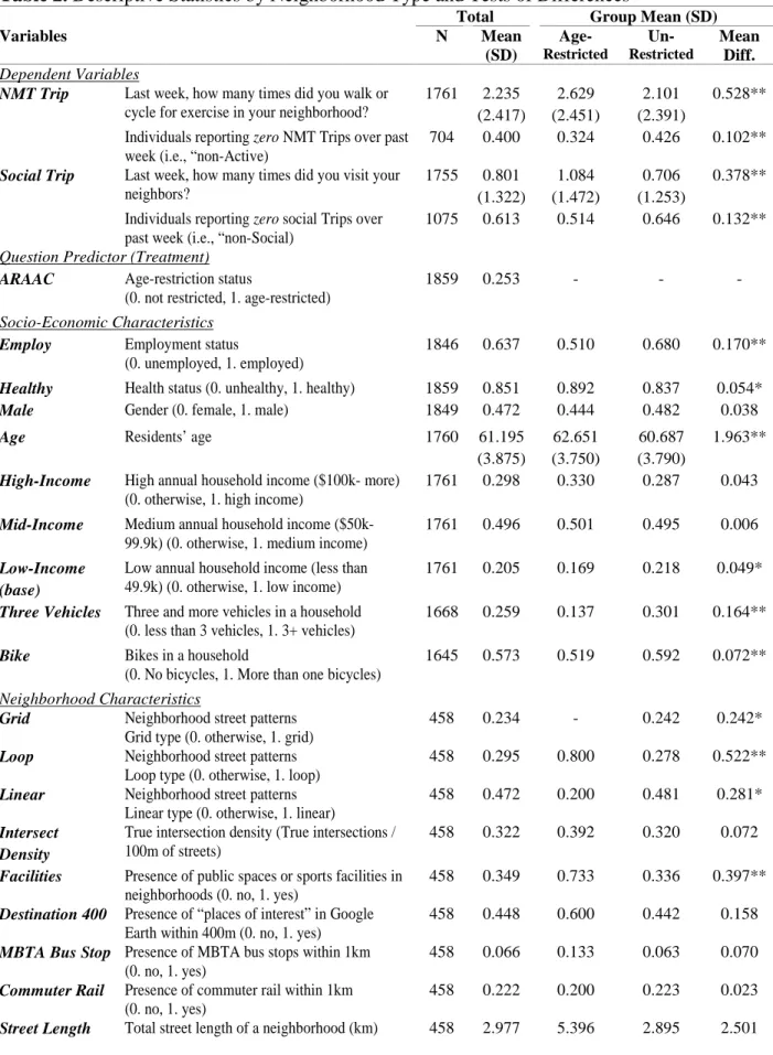
Measures and Descriptive Statistics
Table 2 includes descriptive statistics of key variables, including outcomes of interest, reported weekly: NMT trips, representing recreational walking/biking trips; and social trips, measuring visits to neighbors and representing local social engagement. Respondents in age-restricted neighborhoods have only slightly higher average weekly trip rates for both trip purposes. A large share of individuals in both neighborhood types report making zero NMT and social trips during the week (hereafter these individuals are “non-active” and “non-social”). Un-restricted
neighborhoods have a 10% higher share of non-active and 13% higher share of non-social individuals. Baby boomers residing in age-restricted neighborhoods tend to be less employed, slightly healthier, and slightly older, with fewer owning a bike or more than three cars.
Age-restricted neighborhoods have more local facilities, such as public spaces, and, primarily, loop street patterns. None has grid streets. Nearly 50% of un-restricted neighborhoods have linear street patterns. Other physical characteristics – such as intersection density,
destinations, and proximity to public transportation – do not significantly differ between sampled restricted/un-restricted neighborhoods.
Exploratory factor analysis on the responses to the questions regarding residential preferences led us to hypothesize two latent variables: Pro Walkability, denoting preference for walkable neighborhoods, and Pro Segregation, representing preference for neighborhoods segregated by age and social class. Confirmatory factor analysis confirms this latent structure:
9
fixing the indicators most highly correlated with the two latent variables at 1 for identification, all other indicators significantly contribute to the latent variables. This latent construct serves as a measurement model in the following SEM.8
Figure 1. Three Categories of Neighborhood Street Patterns, Descriptive Diagrams, and Prototypical Examples of the Categorization
Zegras, Lee, Ben-Joseph By Community or Design?
10
Table 2. Descriptive Statistics by Neighborhood Type and Tests of Differences
Total Group Mean (SD)
Variables N Mean (SD) Age-Restricted Un-Restricted Mean Diff. Dependent Variables
NMT Trip Last week, how many times did you walk or cycle for exercise in your neighborhood?
1761 2.235 (2.417) 2.629 (2.451) 2.101 (2.391) 0.528**
Individuals reporting zero NMT Trips over past week (i.e., “non-Active)
704 0.400 0.324 0.426 0.102**
Social Trip Last week, how many times did you visit your neighbors? 1755 0.801 (1.322) 1.084 (1.472) 0.706 (1.253) 0.378**
Individuals reporting zero social Trips over past week (i.e., “non-Social)
1075 0.613 0.514 0.646 0.132**
Question Predictor (Treatment)
ARAAC Age-restriction status
(0. not restricted, 1. age-restricted)
1859 0.253 - - -
Socio-Economic Characteristics
Employ Employment status
(0. unemployed, 1. employed)
1846 0.637 0.510 0.680 0.170**
Healthy Health status (0. unhealthy, 1. healthy) 1859 0.851 0.892 0.837 0.054*
Male Gender (0. female, 1. male) 1849 0.472 0.444 0.482 0.038
Age Residents’ age 1760 61.195 (3.875) 62.651 (3.750) 60.687 (3.790) 1.963**
High-Income High annual household income ($100k- more) (0. otherwise, 1. high income)
1761 0.298 0.330 0.287 0.043
Mid-Income Medium annual household income ($50k- 99.9k) (0. otherwise, 1. medium income)
1761 0.496 0.501 0.495 0.006
Low-Income (base)
Low annual household income (less than 49.9k) (0. otherwise, 1. low income)
1761 0.205 0.169 0.218 0.049*
Three Vehicles Three and more vehicles in a household (0. less than 3 vehicles, 1. 3+ vehicles)
1668 0.259 0.137 0.301 0.164**
Bike Bikes in a household
(0. No bicycles, 1. More than one bicycles)
1645 0.573 0.519 0.592 0.072**
Neighborhood Characteristics
Grid Neighborhood street patterns Grid type (0. otherwise, 1. grid)
458 0.234 - 0.242 0.242*
Loop Neighborhood street patterns Loop type (0. otherwise, 1. loop)
458 0.295 0.800 0.278 0.522**
Linear Neighborhood street patterns Linear type (0. otherwise, 1. linear)
458 0.472 0.200 0.481 0.281*
Intersect Density
True intersection density (True intersections / 100m of streets)
458 0.322 0.392 0.320 0.072
Facilities Presence of public spaces or sports facilities in neighborhoods (0. no, 1. yes)
458 0.349 0.733 0.336 0.397**
Destination 400 Presence of “places of interest” in Google
Earth within 400m (0. no, 1. yes)
458 0.448 0.600 0.442 0.158
MBTA Bus Stop Presence of MBTA bus stops within 1km
(0. no, 1. yes)
458 0.066 0.133 0.063 0.070
Commuter Rail Presence of commuter rail within 1km (0. no, 1. yes)
458 0.222 0.200 0.223 0.023
Street Length Total street length of a neighborhood (km) 458 2.977 5.396 2.895 2.501
Notes: * p<0.05, ** p<0.01, indicating significance levels of difference of means/proportions; 1km = 0.62 mi; 400m = 0.25 mi; 100m = 0.06 mi = 318 ft; - : indicates not applicable; Some totals differ due to missing items in the sample.
11
4. Behavioral Modeling
The large share of zero-reported NMT and social trips (Table 2) indicates censoring – ordinary count models may be inappropriate. We employ a zero-inflated model, allowing zeros to remain in the count model by estimating an individual’s likelihood of being in the “zero” group. Taking recreational NMT trips as an example, a binary logit model estimates the probability of being non-active and active. These probabilities weight the zeros in the count model such that the probability of observing zero for an individual equals the probability of being non-active plus the probability of being active, multiplied by the probability of observing zero in the count model (Jones, 2006) (Fig. 2, Eqs. 1–3). This produces two sets of coefficients. The logit model results indicate the variables’ influence on the likelihood of being non-active; negative coefficients imply a higher probability of being active. The count model estimates trip counts for the active group; positive coefficients mean a higher frequency of recreational NMT trips.
We apply zero-inflated Negative Binomial (ZINB) models9 with SEM that
simultaneously incorporates attitudes possibly affecting residential choice/travel behavior and a residential choice model. Three types of relationships are examined – residential choice,
residential preference, and travel behavior (Fig. 2) – and three models estimated (Appendix provides full results). Model 1 has no control for self-selection. Model 2 attempts to control for individuals’ self-selection for neighborhood physical characteristics by simultaneously
estimating the ZINB model and the latent variable (attitudinal) model’s structural and measurement equations. Model 2 estimates residential preferences conditional upon socio-economic characteristics; thus, travel behavior and residential preferences are endogenous while socio-economic status and neighborhood physical characteristics and age-restricted status are exogenous. Model 3 includes a binary choice model for age-restricted status, assuming people select age-restricted neighborhoods to satisfy community preferences, and that neighborhood and individual characteristics influence age-restricted choice.10 In this case, age-restricted
neighborhood choice, residential preferences, and individual and neighborhood characteristics jointly affect local travel behavior. We estimate the models in Mplus 5.0, using a normal theory maximum likelihood (ML) estimator, and accounting for non-independence among observations from the same household11 (Muthen & Muthen, 2004, 2007).
Zegras, Lee, Ben-Joseph By Community or Design?
12
Figure 2. Path Diagrams and Equations of Three Models That Hypothesize Relationships among the Built Environment, Residential Preference, and Travel Behavior
Path Diagrams Equations
Model 1: Zero-Inflated Negative Binomial Model Without Latent Variables
Model 2: Zero-Inflated Negative Binomial Model With Latent Variables (MIMIC Model)
Model 3: Zero-Inflated Negative Binomial Model With Age-Restricted Neighborhood Choice (Logit) Model
: Zero-Inflated Negative Binomial (ZINB) Model
Logit Model: (Eq. 1) Logit(μ=0) = Xβ+Zγ+Lρ +ε
P(yi = 0) = π = , yi = 0, 1, 2, 3, …
Negative Binomial Model (NB): (Eq. 2) lnY = Xnbβnb+Znbγnb+ Lnbρnb +ζ
P(yi |xnb,i , znb,i , lnb,i) = , yi = 0, 1, 2, 3, …
E(yi |xnb,i , znb,i , lnb,i) = μi =
V(yi |xnb,i , znb,i , lnb,i) = μi (1 + αμi )
Combining the logit and NB models: (Eq. 3) P(yi | xi , zi , yi , xnb,i , znb,i , ynb,i)
=
X Neighborhood Characteristics
Z Socio-economic Characteristics
L Latent Variables (Residential Preference)
Y Count of activities
μ Expected count
π Probability of being in zero-count group
α Variance (Dispersion) parameter
β, γ, ρ Unknown parameters ε, ζ Random disturbance terms
Structural Equation Model (SEM)
: Structural Model (Eq. 4)
L= Zη + ξ, ξ~N(0, ψξ diagonal)
: Measurement Model (Eq. 5)
I = Lλ + δ, δ~N(0, φδ diagonal) Z Socio-economic Characteristics
L Latent Variables (Residential Preference)
I Indicators of L
η, λ Unknown parameters
ξ, δ Random disturbance term
ψ, φ Covariances of random disturbance term
: Age-Restricted Choice (Logit) Model
P(Age-restricted= 1|X,Z,L) = (Eq. 6)
X Neighborhood Characteristics
Z Socio-economic Characteristics
L Latent Variables (Residential Preference)
13 Recreational NMT
The recreational NMT trip results directly support our first hypothesis regarding the effect of age-restricted setting, with some support for neighborhood physical characteristics, but only “bundled” with age-restriction. Figure 3 orients the discussion.
Examine, first, the age-restricted neighborhood choice: after controlling for neighborhood characteristics, age-restricted neighborhoods attract older, higher income people who prefer segregated neighborhoods. Males are less likely to choose age-restriction. Age-restricted
neighborhoods with loop-type streets, higher intersection density, and on-site facilities are more attractive.
Looking at the likelihood of being non-active, neighborhood physical characteristics— loop street type, intersection density, presence of local facilities, total street length—do have an influence, but only indirectly, via the age-restricted choice. Community and design primarily influence the non-active likelihood, with only nearby destinations exerting a significant effect on number of trips among the active. Nearby commuter rail, interestingly, negatively correlates with number of recreational NMT trips.
For individuals, being employed increases the likelihood of being non-active and
decreases the number of NMT trips among the active. Being healthy decreases the likelihood of being non-active. Finally, Walkables” are less likely to be non-active, while
“pro-Segregated” are more likely to be. This latter effect is partly offset by the pro-Segregated choosing age-restricted neighborhoods that, in turn, increase the likelihood of being active.
There is little evidence of self-selection for local NMT trips. While both latent attitudinal constructs significantly affect the choice to be active, they do not change the sign, significance, or magnitude of the age-restricted effect. Age-restricted community settings increase the chance residents will make local recreational NMT trips; perhaps, in part, due to neighborhood physical characteristics. Other than nearby destinations’ effect on NMT trip counts, neighborhood
physical characteristics do not directly affect baby boomers’ being active or number of recreational NMT trips.
Zegras, Lee, Ben-Joseph By Community or Design?
14
Figure 3. Path Diagram and Results of Recreation NMT (Left) and Social Trips (Right) Models
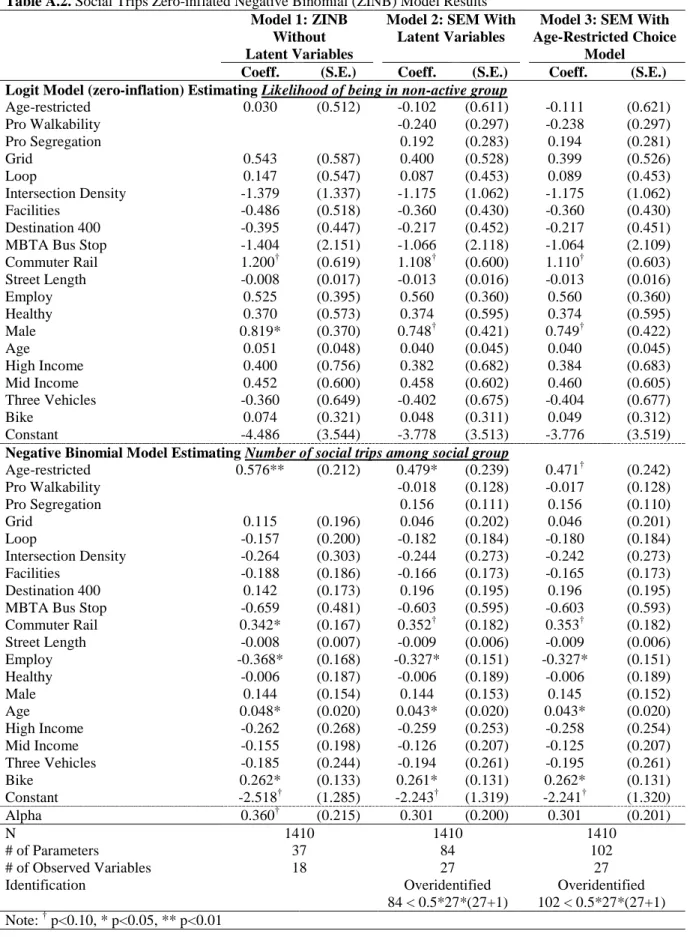
15 Social Trips
The social trip results also only partially support our hypotheses, with distinct, somewhat
counter-intuitive, differences relative to recreational NMT. Age-restricted settings and, indirectly, their bundled physical characteristics exert an uncertain influence on number of social trips. Physical characteristics themselves only modestly (and uncertainly) influence the likelihood of being “social.” Again, Figure 3 guides the discussion.
The same age-restricted choice model as for recreational NMT holds. However, contrary to the NMT case, restricted neighborhoods do not affect being social; among the social, age-restriction increases social trip-making. This result should be viewed with some uncertainty (p-value=0.075) and suggests residential self-selection vis-à-vis social trip-making (compare the significance of the age-restricted neighborhood coefficient from Model 1 to Models 2, 3;
Appendix Table A.2). Those inclined to make more social trips may select age-restricted settings (and, possibly, their physical characteristics) to satisfy social trip-making tendencies. Regarding direct physical effects, street typologies are insignificant. Nearby commuter rail is associated with being social and making more local social trips (p<0.10).
For individuals, being employed increases the likelihood of being non-social.
Unsurprisingly, being employed reduces weekly local social trip-making. Older boomers have greater likelihood of making more social trips. Finally, those preferring segregated
neighborhoods have a higher likelihood of making more social trips.
Social trips offer stronger evidence of self-selection in this study. While age-restricted neighborhoods appear to be associated with more weekly social trips among the socially inclined, statistical support for this effect declines once accounting for attitudes and residential preferences.
5. Implications and Shortcomings
Our findings must be viewed in light of the demographic geography of older adults in metropolitan USA: the majority lives in auto-dependent suburbia. Among our sampled
individuals, for example, 93% of daily reported trips were by automobile, even higher than the automobile mode share for Greater Boston’s baby boomers in 2005 (Hebbert, 2008).11 This study sheds little light on the larger challenges implied. Nonetheless, with respect to two types of local travel activities that may be influenced by suburban neighborhood and community characteristics and play an important role in healthy aging, some influences emerge.
We find modest effects of neighborhood age-restricted status and physical characteristics on weekly recreational NMT and social trip-making. Distinguishing between those who do and do not make a recreational NMT or social trip provides useful information. Eyler et al. (2003), studying adults in the USA, identified three types of walkers: regular, occasional, and never. Occasional and never walkers lacked time for walking and never walkers reported feeling unhealthier, while regular walkers reported more self-confidence and social support for walking. Our recreational NMT results support these findings and suggest a design and community (social network) role: those with a “pro-Walkable” mindset are more likely to be active; the community and, indirectly, design aspects of age-restricted neighborhoods increase residents’ likelihood of being active, after controlling for self-selection. This provides some support for the social ecological model of health promotion – the social-physical setting of the age-restricted
neighborhoods apparently provides a medium for active living (e.g., Wister, 2005). Among the active, however, the neighborhood has no effect on increased recreational NMT trip-making, although nearby destinations do play a role. The age-restricted effect may come from social settings (i.e., community) or other unobserved (or non-comparable) physical characteristics
Zegras, Lee, Ben-Joseph By Community or Design?
16
distinguishing age-restricted from un-restricted suburbs. For example, the age-restricted neighborhoods studied have more local facilities (e.g., clubhouses) than typical suburbs (Table 2); while insignificant in the NMT models, these variables’ effects may be masked by the age-restricted label.
As in the recreational NMT case, some age-restricted physical characteristics
(intersection density, neighborhood facilities, and destinations) indirectly influence social trip-making among the social. In this case, however, residents may be purposefully choosing age-restricted settings and their related design attributes: age-age-restricted settings will not “make” people social, but may attract those with higher social trip-making tendencies.
Our findings indicate the importance of distinguishing between trip types, including when attempting to control for self-selection. The results confirm intuition: an individual may choose a neighborhood to satisfy desired local social activity; this residential choice to satisfy one activity preference might then induce changes in other activities.
Limitations and Future Research
Our results are only directly applicable to a specific demographic, geography, and time-of-year (i.e., April 2008) and may not be generalizable. Even for the specific groups and areas studied, the sampling procedure likely suffers from biases that further limit the results’ validity and generalizability.
The age-restricted effects may be confounded by our not knowing whether some of the un-restricted neighborhoods also have a high share of older adults (i.e., being NORCs), implying similar community structures. This relates to spatial dependence—participation in a particular activity may be influenced by surrounding neighborhoods, including how well “integrated” the neighborhoods are with their surroundings, only crudely proxied here. The age-restricted
neighborhoods’ relative newness may also confound; newer residents13 may still be “exploring” surroundings, effects indistinguishable from the age-restricted status. Over time, such effects may diminish or intensify—an area for further study.
Analytically, complete SEM, simultaneously estimating measurement models of latent attitudinal variables and behavioral (structural) models, represents an important advance. It controls for self-selection based on attitudes and residential choice and allows testing more complex relationships, including direct and indirect effects. The increased modeling
sophistication also comes at a cost—our particular SEM cannot easily reveal relative or marginal effects, only significance and directionality. Furthermore, the design remains cross-sectional, as opposed to temporal (i.e., measuring change). For example, people living in a sociable
community and/or a social-oriented neighborhood may increase, over time, their socializing, which may then change the community (e.g., walking groups) – revealing these dynamics would require longitudinal analysis.
Questions can be raised about the outcomes measured: self-reported recreational NMT trips in the neighborhood and social trips to “neighbors.” Respondents may interpret the extent of “neighborhood” and/or “neighbors” differently. Further, the measures may be weak proxies for outcomes more closely related to healthy aging, such as: minutes of activity per day, health conditions, levels of social engagement, strength of social networks, and/or mental health conditions. Analogously, the validity and reliability of the attitude/preferences questions are uncertain and treating the ordinal Likert-value attitude scores as continuous variables (in the factor analysis), although common practice, may be problematic.
Regarding neighborhood built environment, we attempted “objective” measurement, which may not account for design qualities like sense of safety and human scale (Ewing &
17
Handy, 2009) and may ignore individual perceptions of relevant factors. Again, these perceptions may change over time and be influenced by neighborhood and/or community changes. Enhanced behavioral insights might come from combining qualitative measures of the built environment with “objective” measures.
Further research could examine additional travel behaviors among baby boomers and/or compare suburban and urban baby boomers or age-restricted neighborhoods with non-age-restricted master planned neighborhoods. Such comparisons may reveal whether the modest behavioral effects of age-restricted neighborhoods derive from the community structure, physical features, or their reciprocal interactions. Additional topics worth examining include: the potential to retrofit existing neighborhoods to better serve older adults needs; whether spatial
concentrations of older adults in suburbia increase possibilities for new transportation and/or other older adult services; and the relationship between commuter rail proximity and local trip-making.
Our results indicate the need to better understand how physical and social structures interact to influence older adults’ activities. Overall, however, the relative locations of older adult-oriented neighborhoods need attention. For example, just 13% of the age-restricted
neighborhoods studied are within 1 km of a bus stop and 20% within 1 km of commuter rail. As aging means reduced driving capabilities, this relative automobile-dependency may pose a problem.
6. Conclusion
We studied a neighborhood type catering to older adults—age-restricted, active adult
neighborhoods—and attempted to discern community (e.g., social network) versus physical (e.g., street network) influences on suburban baby boomers’ travel behavior. Using structural
equations models, the analysis attempts to control for self-selection based on attitudes and residential choice, allowing for direct and indirect effects among exogenous and endogenous variables.
The age-restricted neighborhoods attract older, higher income baby boomers who prefer age-segregation. These communities increase the likelihood of boomers being active – i.e., making at least one local recreational NMT trip – but not the number of NMT trips among the active. Physical characteristics have only an indirect effect, by influencing the decision to live in age-restricted settings. In contrast, age-restriction has no effect on being social (i.e., the
likelihood of ever visiting neighbors); among the social, however, age-restriction increases social trip-making, although perhaps due to self-selection. In other words, age-restricted neighborhoods are associated with higher levels of local social activity, but because they attract more socially-inclined residents. The age-restricted effect may stem from a sense of community fostered in age-restricted neighborhoods and/or unobserved or inter-mingling physical characteristics.
Our analysis indicates the importance of distinguishing between trip types when controlling for self-selection in the built environment-travel behavior research. It also suffers from a range of limitations, including generalizability, unknown relative magnitude of effects, and inability to assess impacts over time. While this research offers some insight into the influence of age-restricted neighborhoods on baby boomers’ local travel behaviors, it says nothing about the regional travel patterns of this highly suburbanized, automobile-dependent generation.
Zegras, Lee, Ben-Joseph By Community or Design?
18
Acknowledgments
This work was supported by the New England University Transportation Center, under grant DTRS99-G-0001. The authors would like to thank: Frank Hebbert, who played a major role in survey design, implementation and analysis; Joe Coughlin and Moshe Ben-Akiva, for numerous useful conversations; Kristin Simonson, for assisting in spatial analysis; Lee Carpenter, for editorial assistance; and several anonymous reviewers for detailed and insightful comments and suggestions.
Notes
1
In the USA, the Department of Housing and Urban Development (HUD) uses senior housing, or 55 and older community; residential developer Del Webb refers to Active Adult Communities (Harris
Interactive, 2005); the National Association of Homebuilders suggests Age-Qualified is preferred (Emrath and Liu, 2007).
2
Overall older adult (and age-restricted) household locations in USA: 23% (14%), central cities; 50%, (71%), suburbs; and 27% (15%), outside metro areas (derived from Emrath and Liu, 2007; Tables 1 and 2).
3
A sample selection problem may also exist: among the possible subsamples of baby boomers, factors influencing residential location choice for our age-restricted subsample could also influence behavior. In our case, this problem effectively appears as a form of omitted variable bias (Hebbert, 2008).
4
Based on share of census population in 2000, accumulated over the corresponding census block centroid’s distance from Boston’s central business district.
5
Heudorfer (2005) inventoried (apparently based on a survey of town officials) age-restricted housing in the State, but did not identify individual developments.
6
Problematic responses included: addresses non-geo-locatable or outside the study area (due to mail forwarding); no household survey page; age outside the cohort of interest. Hebbert (2008) provides detail on survey design, implementation, and results.
7
The grid cell approach ensures anonymity –making it impossible to identify the household’s address. The centroid of the 250-meter grid cell serves as the household “location.” Each grid centroid was visually associated to a neighborhood based on primary street characteristics (see Figure 1). Basic data, including roads, parcels, commuter rail, come from MassGIS (http://www.mass.gov/mgis/), although available data were limited. For example, no building footprints for sample neighborhoods could be located and road networks in the newer age-restricted neighborhoods were outdated. We updated missing data using a high resolution aerial photo from ESRI
(http://www.arcgis.com/home/item.html?id=a5fef63517cd4a099b437e55713d3d54) to classify street patterns and compute intersection density. For other neighborhood characteristics (e.g., public spaces, outdoor sports facilities), we used Google Earth’s satellite imagery and “Places” layer, and, in some cases, site plans and age-restricted neighborhoods’ web-pages.
8
Space constraints preclude including the confirmatory factor analysis (CFA). Refer to the Measurement models in Tables A.1 and A.2; full results available upon request.
9
For the NMT and social trip models, the Vuong test indicates that ZINB is preferable to a regular negative binomial; and a likelihood ratio test indicates ZINB is preferable to a zero-inflated Poisson.
10
As mentioned in the sample description, our sample is endogenously stratified. In the age-restricted neighborhood choice (Logit) models, this choice-based sampling results in an inconsistent alternative specific constant, while other coefficients are consistent (Manski and Lerman, 1977). We attempt to correct for this sampling strategy by using weights in the choice model estimation: p/s for households in age-restricted communities and (1-p)/(1-s) for households from un-restricted communities, where p is the probability of a household living in an age-restricted community from the population and s is the
proportion of households from our sample living in an age-restricted community. As a value for p is not available, we use 3.2% (Emrath and Liu, 2007). We test the sensitivity of results to this value by
19
estimating the models with p = 1% and 6% (reasonable upper and lower bounds); the results do not vary substantively. Full sensitivity analyses are available upon request.
11
We sampled households but model individuals, thus need to account for potential correlation of
behavior among same-household individuals (i.e., intra-class correlation). One option MPlus provides for dealing with this issue is correcting standard errors (SEs); using this approach, the SEs in Tables 3 and 4 are “corrected.” Our approach may also have intra-class correlation among households from the same neighborhood, indicating the need for a multi-level SEM ZINB model. We leave this approach for future research.
12
The differences may partially result from under-counting in our survey; however, note that the
boomers’ automobile mode share (89%) from NHTS (2005) is for all of Greater Boston, while our value is suburban only, so that our result does not seem unlikely.
13
Residents of age-restricted neighborhoods report having lived there on average for 5 years, compared to 19 years for un-restricted neighborhoods (Hebbert, 2008).
References
Ahrentzen, S. (2010) On Their Own Turf: Community Design and Active Aging in a Naturally Occurring Retirement Community, Journal of Housing for the Elderly, 24(3/4), pp. 267– 290
Alfonzo, M., Boarnet, M., Day, K., Mcmillan, T. and Anderson, C. (2008) The Relationship of Neighbourhood Built Environment Features and Adult Parents' Walking, Journal of Urban Design, 13(1), pp. 29–51.
Baran, P., Rodríguez, D. and Khattak, A. (2008) Space Syntax and Walking in a New Urbanist and Suburban Neighborhoods, Journal of Urban Design, 13(1), pp. 5–28.
Ben-Akiva, M., Walker, J., Bernardino, A. T., Gopinath, D. A., Morikawa, T., and Polydoropoulou, A. (1999) Integration of Choice and Latent Variable Models, in
International Association of Traveler Behavior Research (IATBR), proceedings from the 1997 Conference in Austin, Texas.
Berke, E.M., Gottlieb, L.M., Moudon, A.V., and Larson, E.B. (2007a) Protective Association Between Neighborhood Walkability and Depression in Older Men, Journal of the American Geriatrics Society, 55, pp. 526–533.
Berke, E.M., Koepsell, T.D., Moudon, A.V., Hoskins, R.E., and Larson, E.B. (2007b)
Association of the Built Environment with Physical Activity and Obesity in Older Persons, American Journal of Public Health, 97(3), pp. 486–492.
Blechman, A. (2008) Leisureville: Adventures in America’s Retirement Utopias. New York, NY: Atlantic Monthly Press
Cao, X., Handy, S. and Mokhtarian, P. (2006) The Influences of the Built Environment and Residential Self-Selection on Pedestrian Behavior: Evidence from Austin, TX,
Transportation, 33(1), 2006, pp. 1–20.
Cao, X., Mokhtarian, P. and Handy, S. (2010) Neighborhood Design and the Accessibility of the Elderly: An Empirical Analysis in North California, International Journal of Sustainable Transportation, 4, pp. 347–371.
Champion, A.G. (2001) A Changing Demographic Regime and Evolving Polycentric Urban Regions: Consequences for the Size, Composition and Distribution of City Populations, Urban Studies, 38(4), pp. 657–677.
Chapman, N.J. and Beaudet, M. (1983) Environmental Predictors of Well-Being for At-risk Older Adults in a Mid-sized City, Journal of Gerontology, 38(2), pp. 237–244.
Chaskin, R.J. (1995) Defining Neighborhood: History, Theory, and Practice. Chicago: The Chapin Hall Center for Children, University of Chicago,
Zegras, Lee, Ben-Joseph By Community or Design?
20
Coughlin, J. (2007) Disruptive Demographics, Design, and the Future of Everyday Environments, Design Management Review, 18(2), pp. 53–59.
Cvitkovich, Y. and Wister, A. (2001) The Importance of Transportation and Prioritization of Environmental Needs to Sustain Well-Being Among Older Adults, Environment and Behavior, 33(6), pp. 809–829.
DiPietro, L. (2001) Physical Activity in Aging: Changes in Patterns and Their Relationship to Health and Function, Journal of Gerontology A, 56(2), pp. 13–22.
Emrath, P. and Liu, H.F. (2007) The age-qualified active adult housing market. Washington, DC: National Association of Home Builders.
Ewing, R. and Handy, S. (2009) Measuring the Unmeasurable: Urban Design Qualities Related to Walkability, Journal of Urban Design, 14(1), pp. 65–84.
Eyler, A. Brownson, R., Bacak, S., and Housemann, R. (2003) Epidemiology of Walking for Physical Activity in the United States, Medicine & Science in Sports & Exercise, 35(9), pp. 1529–1536
Flynn, T.E., and Boenau, A.E. (2007) Trip Generation Characteristics of Age-Restricted Housing, ITE Journal, 77(2), pp. 30–37.
Giles-Corti, B., Broomhall, M.,Knuiman, M. Collins, C., Douglas, K., Ng, K., Lange, A. and Donovan, R. (2005) Increasing Walking: How Important is Distance to, Attractiveness, and Size of Public Open Space? American Journal of Preventive Medicine, 28(2S2), pp. 169– 176.
Giles-Corti, B., and Donovan, R. (2002) The Relative Influence of Individual, Social and Physical Environment Determinants of Physical Activity, Social Science & Medicine, 54(12), pp. 1793–1812.
Golob, T. (2003) Structural equation modeling for travel behavior research, Transportation Research Part B, 37(1), pp. 1–25.
Grant, J., and Mittelsteadt, L. (2004) Types of gated communities, Environment and Planning B, 31, pp. 913–930.
Hebbert, F. (2008) Local Travel Habits of Baby Boomers in Suburban Age-restricted
Communities, Masters Thesis submitted to the Department of Urban Studies and Planning, Massachusetts Institute of Technology, Cambridge.
Heudorfer, B. (2005) Age Restricted Active Adult Housing in Massachusetts, Boston MA: Citizens’ Housing and Planning Association, June.
Hunt, M. E. and Gunter-Hunt, G. (1985) Naturally Occurring Retirement Communities, Journal of Housing for the Elderly, 3(3/4), pp. 3–22.
Huston, S., Evenson, K., Bors, P. and Gizlice, Z. (2003) Neighborhood Environment, Access to Places for Activity, and Leisure-time Physical Activity in a Diverse North Carolina Population, American Journal of Health Promotion, 18, pp. 158–169.
Jones, A.J. (2005) Applied Econometrics for Health Economists: A Practical Guide, 2nd Edition, York, UK: Office of Health Economics.
Joseph, A., and Zimring, C. (2007) Where Active Older Adults Walk: Understanding the Factors Related to Path Choice for Walking Among Active Retirement Community Residents, Environment and Behavior, 39(1), pp. 75–105.
Kennedy, D.J., and Coates, D. (2008) Retirement Village Resident Satisfaction in Australia: A Qualitative Enquiry, Journal of Housing for the Elderly, 22(4), pp. 311–334.
21
King, W., Brach, J., Belle, S., Killingsworth, R., Fenton, M. and Kriska, A.M. (2003) The Relationship between Convenience of Destinations and Walking Levels in Older Women, American Journal of Health Promotion, 18(1), pp. 74–82.
Kweon, B.-S., Sullivan, W., and Wiley, A. (1998) Green Common Spaces and the Social Integration of Inner-City Older Adults, Environment and Behavior, 30(6), pp. 832–858. Lawton, M.P., Nahemow, L., and Teaff, J. (1975) Housing Characteristics and the Well-Being of
Elderly Tenants in Federally Assisted Housing, Journal of Gerontology, 30(5), pp. 601– 607.
Lee, C., and Moudon, A.V. (2006) Correlates of Walking for Transportation or Recreation Purposes, Journal of Physical Activity and Health, 3(S1), pp. S77–S98.
Maat, K., Wee, B. van and Stead, D. (2005) Land use and travel behaviour: expected effects from the perspective of utility theory and activity-based theories, Environment and Planning B, 32, pp. 33–46.
Mokhtarian, P. and Cao, X. (2008) Examining the impacts of residential self-selection on travel behavior: A focus on methodologies, Transportation Research B, 42(3), pp. 204–228. Manski, C. and Lerman, S. (1977) The Estimation of Choice Probabilities from Choice-Based
Samples, Econometrica, 45(8), pp.1977-1988.
Moudon, A.V., Lee, C., Cheadle, A., Garvin, C., Johnson, D., Schmid, T., Weathers, R., and Lin, L (2005) Operational Definition of Walkable Neighborhood, Journal of Physical Activity and Health, 3(S1), pp. S99–S117.
Muthen, L., and Muthen, B. (2004). Mplus Technical Appendices. Los Angeles: Muthen & Muthen.
Muthen, L., and Muthen, B. (2007). Mplus User's Guide. 5th Edition. Los Angeles: Muthen & Muthen.
Nagel, C., Carlson, N. Bosworth, M., and Michael, Y. (2008) The Relation between
Neighborhood Built Environment and Walking Activity among Older Adults, American Journal of Epidemiology, 168(4), pp. 461–468.
Owen, N., Humpel, N., Leslie, E., Bauman, A. and Sallis, J.F. (2004) Understanding
Environmental Influences on Walking: Review and Research Agenda, American Journal of Preventive Medicine, 27(1), pp. 67–76.
Phillipson, C., Leach, R., Money, A., and Biggs, S. (2008) Social and Cultural Constructions of Ageing: The Case of the Baby Boomers, Sociological Research Online
13(3)5://www.socresonline.org.uk/13/3/5.html.
Rodriguez, D., Khattak, A. and Kelly, E. (2006) Can New Urbanism Encourage Physical Activity? Comparing a New Urbanist Neighborhood with Conventional Suburbs, Journal of the American Planning Association, 72(1), pp. 43–54.
Rosenbloom, S. (2003) The Mobility Needs of Older Americans: Implications for Transportation Reauthorization, Transportation Reform Series, Washington, D.C.: The Brookings
Institution.
Saelens, B., and Sallis, J. (2003) Neighborhood-Based Differences in Physical Activity: An Environment Scale Evaluation, American Journal of Public Health, 93(9), pp. 1552–1558. Sallis, J., and Owen, N. (1996) Ecological models, Health Behavior and Health Education:
Theory, Research, and Practice, (Glanz, K., Rimer, B.K. and Lewis, F.M., eds.), Second Edition, San Francisco: Jossey-Bass.
Zegras, Lee, Ben-Joseph By Community or Design?
22
Schmöcker, J.-D., Quddus, M.A., Noland, R.B., and Bell, M.G.H. (2005) Estimating Trip Generation of Elderly and Disabled People: Analysis of London Data, Transportation Research Record No. 1924, pp. 9–18.
Wachs, M. (1979) Transportation for the elderly: Changing lifestyles, changing needs. Berkeley, CA: University of California Press.
Wellman, B. (2005) Community: From Neighborhood to Network, Communications of the ACM, 48(10), pp. 53–55.
Wister, A. (2005) Baby boomer health dynamics: How are we aging? Toronto, ON: University of Toronto Press.
Wretstrand, A., Svensson, H., Fristedt, S., and Falkmer, T. (2009) Older people and local public transit: Mobility effects of accessibility improvements in Sweden, Journal of Transport and Land Use, 2(2), pp. 49–65.
Yang, H.-Y. and Stark, S.L.(2010) The Role of Environmental Features in Social Engagement Among Residents Living in Assisted Living Facilities, Journal of Housing For the Elderly, 24(1), pp. 28–43.
23
Table A.1. Recreational NMT Trips Zero-inflated Negative Binomial (ZINB) Model Results Model 1: ZINB
Without Latent Variables
Model 2: SEM With Latent Variables
Model 3: SEM With Age-Restricted Choice
Model Coeff. (S.E.) Coeff. (S.E.) Coeff. (S.E.) Logit Model (zero-inflation) Estimating Likelihood of being in non-active group
Age-restricted -0.519* (0.244) -0.602* (0.249) -0.610* (0.250) Pro Walkability -0.212* (0.098) -0.213* (0.097) Pro Segregation 0.210* (0.095) 0.208* (0.094) Grid -0.172 (0.182) -0.188 (0.181) -0.188 (0.181) Loop 0.059 (0.179) 0.055 (0.181) 0.056 (0.181) Intersection Density -0.296 (0.422) -0.211 (0.413) -0.210 (0.413) Facilities -0.027 (0.165) -0.010 (0.166) -0.009 (0.166) Destination 400 0.017 (0.160) 0.060 (0.161) 0.060 (0.161) MBTA Bus Stop -0.166 (0.283) -0.092 (0.284) -0.093 (0.284) Commuter Rail -0.053 (0.180) -0.041 (0.184) -0.041 (0.184) Street Length 0.004 (0.009) 0.002 (0.009) 0.002 (0.009) Employ 0.578** (0.166) 0.606** (0.167) 0.606** (0.167) Healthy -0.743** (0.196) -0.788** (0.196) -0.788** (0.196) Male 0.027 (0.134) -0.048 (0.137) -0.048 (0.137) Age 0.011 (0.020) 0.012 (0.020) 0.012 (0.020) High Income -0.129 (0.205) -0.102 (0.207) -0.102 (0.207) Mid Income 0.053 (0.190) 0.067 (0.190) 0.066 (0.190) Three Vehicles -0.096 (0.164) -0.165 (0.167) -0.165 (0.167) Bike -0.449** (0.146) -0.430** (0.148) -0.430** (0.148) Constant -0.466 (1.295) -0.509 (1.311) -0.511 (1.311)
Negative Binomial Model Estimating Number of NMT trips among active group
Age-restricted 0.053 (0.087) 0.078 (0.087) 0.080 (0.088) Pro Walkability -0.032 (0.038) -0.031 (0.038) Pro Segregation -0.037 (0.036) -0.037 (0.036) Grid 0.001 (0.069) 0.007 (0.069) 0.007 (0.069) Loop -0.034 (0.068) -0.029 (0.068) -0.029 (0.068) Intersection Density -0.050 (0.115) -0.052 (0.113) -0.052 (0.113) Facilities 0.000 (0.066) 0.010 (0.066) 0.010 (0.066) Destination 400 0.128 (0.060) 0.139* (0.060) 0.139* (0.060) MBTA Bus Stop 0.101 (0.108) 0.099 (0.105) 0.099 (0.105) Commuter Rail -0.163* (0.068) -0.177* (0.068) -0.177* (0.068) Street Length 0.001 (0.003) 0.000 (0.003) 0.000 (0.003) Employ -0.227** (0.055) -0.234** (0.056) -0.234** (0.056) Healthy 0.065 (0.078) 0.063 (0.078) 0.063 (0.078) Male -0.020 (0.049) -0.022 (0.049) -0.022 (0.049) Age -0.004 (0.007) -0.003 (0.007) -0.003 (0.007) High Income -0.015 (0.074) -0.014 (0.074) -0.014 (0.074) Mid Income -0.035 (0.071) -0.041 (0.071) -0.041 (0.071) Three Vehicles -0.038 (0.063) -0.046 (0.062) -0.046 (0.062) Bike 0.034 (0.055) 0.030 (0.055) 0.030 (0.055) Constant 1.569** (0.422) 1.552** (0.422) 1.552** (0.422) Alpha 0.089** (0.024) 0.088** (0.024) 0.088** (0.024) N 1456 1456 1456 # of Parameters 37 84 102 # of Observed Variables 18 27 27 Identification Overidentified 84 < 0.5*27*(27+1) Overidentified 102 < 0.5*27*(27+1) Note: † p<0.10, * p<0.05, ** p<0.01