I
CO
2and N
2O dynamics in
the ocean
–sea ice–atmosphere system
Thesis submitted by Marie KOTOVITCH
in fulfilment of the requirements of the PhD Degree in sciences (“Docteur en
sciences”)
Academic year 2018-2019
Supervisors: Doctor Bruno DELILLE (Université de Liège)
and Professor Jean-Louis TISON (Université Libre de Bruxelles)
III
ABSTRACT
Greenhouse gases such as carbon dioxide (CO2), methane (CH4) and nitrous oxide
(N2O) are well known to be indirectly responsible for many changes in the sea ice
cover in the polar regions, as these regions are sensitive to global warming. The objective of this manuscript is to look at the two climatic gases addressed (CO2 and
N2O) and their behaviour in the ocean – sea ice – atmosphere system in the actual
warming climate, thus more specifically in the Arctic.
On the one hand, the dynamic of CO2 has been studied through artificial sea ice
during an experiment performed on two series of mesocosms: one was filled with seawater (SW) and the other one with seawater with added filtered humic-rich river water (SWR). The addition of river water almost doubled the dissolved organic carbon (DOC) concentration in SWR and consequently affected the partial pressure of carbon dioxide (pCO2). This experiment supports previous observations
showing that the pCO2 in sea ice brines is generally higher in Arctic sea ice
compared to that from the Southern Ocean, especially in winter and early spring. Indeed, DOC is larger in the Arctic seawater: higher concentrations of DOC would be reflected in a greater DOC incorporation in sea ice, enhancing bacterial respiration, which in turn would increase the pCO2 in the ice. Within the same
experiment, air–ice CO2 fluxes were measured continuously using automated
chambers from the initial freezing of a sea ice cover until its decay. Cooling seawater prior to sea ice formation acted as a sink for atmospheric CO2, but as soon
as the first ice crystals started to form, sea ice turned to a source of CO2, which
lasted throughout the whole ice growth phase. Once ice decay was initiated, sea ice shifted back again to a sink of CO2. Combining measured air–ice CO2 fluxes with
the pCO2 in the air and sea ice, we determined two strongly different gas transfer
coefficients of CO2 at the air–ice interface between the growth and the decay
IV
In the other hand, we present in this work the first winter to spring N2O
observations in the sea ice and the upper ocean of the western Nansen Basin (Arctic Ocean). In the seawater, a general N2O undersaturation with respect to the
atmosphere was identified at the surface, with a clear enrichment north of 82°N originating from the water masses passing through the Arctic polar circle. We show that the main source of N2O enrichment originates from the East Siberian Arctic
Shelf, a key place for benthic denitrification and sea ice formation rejecting brine – including N2O – in the seawater. Sea ice shows N2O oversaturation throughout
winter and spring in both first-year (FYI) and second-year ice (SYI). Further, SYI, with expected lower salinity than FYI, is enriched in N2O compared to the dilution
curve for salinity. This non-conservative N2O content of SYI with salinity is likely
due to (i) SYI formation further east than FYI, (ii) in situ biological activity, (iii) flushing of N2O-rich ice surface meltwater (i.e. brine skim) through decaying FYI
and (iv) strongly reduced permeability in SYI. Finally, we suggest that the high N2O concentrations observed in the snow cover results from a combination of brine
rejection at the top of the ice (brine skim) and chemical N2O production (under the
V
RÉSUMÉ
La glace de mer, principalement située dans les régions polaires, est un milieu sensible au réchauffement climatique, et de manière accentuée en Arctique où la réduction significative de l’étendue et de l’épaisseur de la glace de mer sont actuellement en cours. Ce réchauffement est causé par des gaz à effet de serre comme le dioxyde de carbone (CO2), le méthane (CH4) et l’oxyde nitreux (N2O), dont
les concentrations augmentent avec l’industrialisation. Ces mêmes gaz sont par ailleurs incorporés dans les saumures liquides et les poches gazeuses de la glace de mer, et par conséquent, leurs concentrations se trouvent affectées par les fluctuations biogéochimiques de la glace de mer. L’objectif de cette thèse est d’étudier la dynamique de deux de ces gaz biologiquement actifs – le CO2 et le N2O
– au sein de la glace de mer et aux interfaces avec l’océan et l’atmosphère.
La dynamique du CO2 a été étudiée lors d’une expérience sur de la glace de mer
artificielle présentant deux types de mésocosmes : l’un rempli avec de l’eau de mer (SW), l’autre rempli avec un mélange d’eau de mer et de rivière (SWR). L’addition d’eau de rivière a presque doublé la concentration en carbone organique dissous (DOC) dans le SWR, affectant la pression partielle en CO2 (pCO2). Cette expérience
confirme d’autres études montrant que la pCO2 mesurée dans les saumures de la
glace de mer est plus élevée en Arctique qu’en Antarctique. En effet, l’Océan Arctique a un contenu en DOC plus important ; une plus grande concentration en DOC dans l’eau de mer mène à une plus grande incorporation de DOC dans la glace de mer lors de sa formation, renforçant la respiration bactérienne qui, en retour, augmente la pCO2 dans la glace. Lors de cette même expérience, des mesures en
continu de flux de CO2 air–glace ont été réalisées, de la formation à la fonte de la
glace de mer. Le refroidissement de l’eau de mer a d’abord agi comme un puits de CO2 pour l’atmosphère, une situation qui s’est inversée lors de la formation des
premiers cristaux de glace, devenant alors une source de CO2 pour l’atmosphère
durant toute la période de croissance de la glace. Enfin, lors de la fonte de la glace, celle-ci s’est repositionnée en puits de CO2 envers l’atmosphère. En combinant les
VI
coefficients de transfert de gaz distincts ont été déterminés ; K = 2.5 mol m−2 d−1
atm−1 pour la phase de croissance et K = 0.4 mol m−2 d−1 atm−1 pour la phase de
fonte.
Quant à la dynamique du N2O, celle-ci a été étudiée à travers un set de données
innovant de mesures de N2O réalisées sur une période de six mois dans la glace et
l’eau de mer de l’Océan Arctique, à l’ouest du Basin de Nansen. Une sous-saturation générale est observée à la surface de l’océan par rapport à l’atmosphère, majoritairement due à l’origine Atlantique de ces masses d’eaux. Cependant un enrichissement en N2O est observé au nord de 82°N, également dû à l’origine de
ces masses d’eaux, qui elles proviennent du plateau arctique de la Sibérie orientale, un lieu intense de dénitrification benthique et de formation de glace de mer, rejetant d’importantes quantités de sels et de gaz dans l’eau sous-jacente. Les mesures dans la glace de mer montrent une sursaturation tout au long de l’étude, dans les deux types de glace étudiées ; celle de première année (FYI) et celle de seconde année (SYI). Cette dernière présente des salinités plus faibles du au lessivage des saumures qui a lieu en fin du premier cycle de croissance, cependant les concentrations en N2O sont similaires à celles de la FYI. Ce comportement non
conservatif par rapport à la salinité peut être dû : (i) à la formation plus à l’est de la SYI, (ii) à de la potentielle activité biologique, (iii) au lessivage de la surface de la glace enrichie en N2O (iv) à la faible perméabilité de la SYI. Enfin, il est suggéré
que les fortes concentrations en N2O rencontrées à la surface de la glace sont dues
au rejet des saumures vers la surface, combiné à un processus chimique de production de N2O.
VII
ACKNOWLEDGEMENTS
Cette thèse s’est construite sur cinq années ponctuées de cinq missions en Arctique, de conférences autour du monde, de rencontres formidables et de projets personnels divers. On pourrait presque croire que tout s’est passé sans difficultés… Mais ce n’est qu’un leurre ! Je n’y serais pas arrivée sans l’aide de nombreuses personnes, ni sans les collaborations reprises ci-dessous.
J’aimerais tout d’abord remercier mes deux promoteurs, Bruno, et Jean-Louis, qui m’ont montré la beauté de la recherche fondamentale (et sa réalité, avec ses défauts), et qui m’ont intégrée dans leur équipe respective.
Bruno, ta passion pour la recherche, ton application dans les tâches les plus diverses, ta patience, ton humanisme, et par-dessus tout, ta foi en moi (entre autre en me laissant partir seule à 5 reprises sur le terrain!) sont toutes des qualités qui m’ont guidée dans mes projets et aidée à rebondir après chaque coup de mou. Je ne sais comment te remercier, et je ne le ferais sûrement jamais assez pour compenser le temps que tu m’as consacré, mais ce dernier mot atténuera peut-être ma dette… Merci !
Jean-Louis, même si les échanges étaient moins fréquents avec toi, ils étaient compensés par leur intensité ! Je ne suis jamais sortie d’une réunion avec toi sans la tête pleine à craquer. L’énergie et la force mentale que tu dégages m’ont permises d’aller chaque fois un peu plus loin dans mes recherches. Je te dois un immense Merci !
I want to thank the members of my jury: Lei Chou and Alberto Borges that were part of my comitee and guided me during 5 years, Frank Dehairs for your contribution to the reading and defense, and Liyang Zhan for inviting me in your Institute more than 2 years ago, and now coming from so far, to support my contribution to the scientific research.
Of course, I would also like to thank the F.R.S.-FNRS and the funding David and Alice Van Buuren with the foundation Jaumotte-Demoulin for all the financial supports.
VIII
Fanny, c’est déjà ton tour, parce que tu prends trop de place dans l’histoire de ma thèse. En 5 ans j’ai passé plus de temps avec toi qu’avec aucune autre personne. J’estime le nombre d’heure que nous avons passé ensemble à plus de 3000, quand même. Mais tu sais comme moi que nos aventures ne s’arrêtent pas là, qu’on va continuer à cumuler ces heures même si ce ne sera pas sur une motoneige, ni sur le dos d’un renne.
Caro, une belle rencontre, et une amitié qui s’est créée et qui ne s’arrêtera pas aux murs du bâtiment DC. Merci pour ton soutien et tes mots justes et apaisants dans les moments de déprime, elle nous en aura fait voir cette thèse.
Vio, une histoire d’enfance, de baguettes magiques, de festivals de youkous, d’unif et puis de glaces ! Merci pour les moments partagés et pour ceux qu’on partagera (il semblerait que nos chemins de vies sont voués à se croiser régulièrement). Seb, mon parrain de thèse, mon mentor, mon guide,… Tu m’as donné tous les petits trucs qui rendent une thèse plus agréable, de comment soumettre un papier à comment se faire des potes en conférences et terminer ses soirées à l’Absinthe en plein milieu de Prague. Je te dois un grand MERCI, tu peux compter sur moi pour te rendre la pareille.
Puis il y a OPTIMISM ! Merci Martin, Tonio, Fred et bien sûr Stefano, même si la probabilité qu’il lise ses lignes dans son fauteuil qui lui sert de lit en hiver soit faible… OUFTI dit-on à Litch, c’était pas rien ces campagnes roots au Spitzberg, ce camping sauvage à faire la ronde aux ours, ces heures de motoneige dans la f****** moraine. Alors je vous dis Merci à vous et à LOCEAN, pour m’avoir laissé une place dans votre team de faux frouz, pour m’avoir hébergé, pour le dernier goal contre le Japon, pour le canard laqué, et pour tous les autres beaux souvenirs que vous avez générés en moi…
En parlant de Liège, je tiens à remercier Marc, Fleur, Gersande et Willy pour leur agréable compagnie, ainsi que leur aide précieuse en laboratoire.
Saida, merci d’avoir enjoué mes journées. I thank you in English for these 6 years spend by yours side (now that you understand this language better ).
IX
Claire, ta présence m’a fait beaucoup de bien au laboratoire, tu sais trouver les mots pour rassurer et redonner confiance, je te remercie pour cela et pour toutes les petites choses qu’on a partagé ces 5 dernières années.
Sans oublier Odile, Gauthier, François, Florian et Morgane car leur présence et leurs conseils (personnels ou professionnels) m’ont portés et motivés à terminer cette thèse.
I also would like to thank Frank, and the rest of the glacio team: Sophie, Lionel, Boris, Brice, Célia, Jiayun, Sainan, Mana, Cons, Lars, Sarah, for all they did for me, the precious time we had during the lunch or at the Pickwick!
I can’t forget the people from Norwich for their hospitality and their perseverance with the sea ice chamber. And thanks to the BEPSII’s community for the great discussions we had all around the world! I would like to add a little note for people that marked my PhD: Sirii, Anna and Daiki, thanks a lot for you presence and your help at any time.
I want to add that this study was supported by the European Community’s 7th Framework Programme through the grant to the budget of the Integrated Infrastructure Initiative HYDRALAB-IV, Contract No. 261520 and Hamburg Ship Model Basin (HSVA) for their logistical support. N-ICE survey was supported by the Norwegian Polar Institute’s Centre for Ice, Climate and Ecosystems (ICE). Il y a aussi et surtout mes amis d’horizons divers, et les habitants des 3 colocs par lesquelles je suis passée depuis mes débuts dans la recherche (Temple, Brukot et Jupiter), merci à tous de m’avoir supportée dans toutes mes phases de thèse ! Enfin, mon papa et mon compagnon, les deux hommes de ma vie. Merci pour tout l’amour que vous m’avez donné, et pour la confiance que vous avez en moi. Je me rends de plus en plus compte à quel point cette confiance (bien dosée) élève les hommes et leur permet de dépasser leurs limites. Je tâcherai de faire de même avec mon entourage (je ne peux m’empêcher de penser à mes futurs élèves), afin qu’eux aussi puissent faire aboutir leurs projets et réaliser leurs rêves.
XI TABLE OF CONTENTS ABSTRACT... I RÉSUMÉ ... V ACKNOWLEDGEMENT ... VII TABLE OF CONTENTS ... XI LIST OF ABBREVIATIONS ... XV I. CHAPTER I: Introduction ... 1 I.1. Motivation ... 1
I.2. Thesis outlines ... 3
II. CHAPTER II: State of the art ... 5
II.1. The climatic relevance of CO2 and N2O in the polar marine environment ... 5
II.1.1. A quick look at the global warming main cause and feedback on sea ice melt ... 5
II.1.2. A positive feedback on sea ice melt: the decreasing albedo ... 5
II.1.3. Atmospheric relevance of CO2 and N2O ... 6
II.1.4. The marine cycle of carbon and nitrogen ... 8
II.2. From a free-ice to an ice-covered seawater ... 10
II.2.1. Sea ice formation conditions and its resulting structure ... 10
II.2.2. Sea ice growth ... 12
II.2.3. Sea ice texture ... 12
II.3. The significant role of salts in sea ice ... 16
II.3.1. What does salinity profiles state ... 16
II.3.2. Brine volume fraction and brine salinity relationships ... 17
II.3.3. Brine concentration and dilution ... 19
II.3.4. Permeability threshold for liquid brine ... 19
II.3.5. Desalinisation processes ... 20
II.4. Gas bubbles within sea ice ... 23
II.4.1. Gas bubbles formation ... 23
II.4.2. Total gas content ... 24
II.4.3. Permeability thresholds for gas bubbles ... 24
II.5. Gas transport in sea ice ... 26 II.5.1. Brine and bubbles dynamics from sea ice growth to sea ice decay 26
XII
II.5.2. Gas diffusion ... 27
II.6. CO2 dynamics within the ice and at the interfaces ... 28
II.6.1. Overview of the carbonate chemistry system ... 28
II.6.2. The carbonate system within sea ice ... 29
II.6.3. CO2 exchanges at the sea ice–seawater interface ... 31
II.6.4. CO2 fluxes at the atmosphere–sea ice interface ... 31
II.7. N2O dynamics within the ice and the seawater ... 33
II.7.1. Processes controlling N2O concentration ... 33
II.7.2. The N2O dynamic in the Arctic Ocean ... 35
II.7.3. The N2O dynamic in sea ice ... 37
II.8. The Arctic Ocean ... 39
II.8.1. Arctic Ocean topography ... 39
II.8.2. Arctic Ocean circulation ... 40
III. CHAPTER III: The impact of dissolved organic carbon and bacterial respiration on pCO2 in experimental sea ice ... 43
Abstract ... 44
III.1. Introduction ... 44
III.2. Material and methods... 45
III.2.1. Experimental setting, and sampling routine and initial conditions .. ... 45
III.2.2. Brine volume fraction and Raleigh number ... 46
III.2.3. DOC and DON ... 46
III.2.4. Bacterial respiration ... 46
III.2.5. pCO2 ... 46
III.2.6. TA and DIC ... 47
III.2.7. Differences between the SW and SWR series and statistical tests 47 III.3. Results ... 47
III.3.1. Physical sea ice conditions ... 47
III.3.2. DOC and DON ... 47
III.3.3. Bacterial activity ... 48
III.3.4. DIC7 ... 49
III.3.5. pCO2 ... 49
III.4. Discussion ... 49
XIII
III.4.2. Similarities of DIC and pCO2 in ice in the SW and SWR mesocosms
... 51
III.4.3. Differences of DIC and pCO2 in ice between the SW and SWR mesocosms ... 52
III.4.4. Modelling the impact of bacterial respiration on pCO2 in ice ... 53
III.5. Conclusion and large scale implications ... 56
IV. CHAPTER IV: Air–ice carbon pathways inferred from a sea ice tank experiment ... 57
Abstract ... 58
IV.1. Introduction ... 58
IV.2. Methods ... 59
IV.2.1. Experimental setting ... 59
IV.2.2. Ice pCO2 at high vertical resolution ... 59
IV.2.3. Total alkalinity ... 60
IV.2.4. Dissolved inorganic carbon ... 60
IV.2.5. Seawater pCO2 ... 60
IV.2.6. Air–ice CO2 fluxes ... 60
IV.2.7. Assessment of the precision of derived variables ... 61
IV.2.8. Modelling air–ice CO2 fluxes ... 61
IV.3. Results and discussion... 62
IV.3.1. Total alkalinity ... 63
IV.3.2. CO2 exchange at the air–ice interface ... 63
IV.3.3. Determination of a gas transfer coefficient for CO2 in artificial sea ice ... 65
IV.3.4. Model sensitivity experiments on the CO2 transport pathways through sea ice ... 66
IV.3.5. Synthesis ... 67
IV.4. Conclusions ... 69
V. CHAPTER V: Winter to spring ocean̶̶̶̶̶̶̶̶̶̶̶̶̶̶̶̶ sea ice̶̶̶̶ atmosphere N2O partitioning in the Arctic Ocean (north of Svalbard) ... 71
Abstract ... 72
V.1. Introduction ... 72
V.2. Sampling area ... 75
V.3. Material and methods... 77
V.3.1. Seawater sampling (on-ice and ship rosette) ... 77
XIV
V.3.3. Snow sampling ... 79
V.3.4. Nutrients and dissolved oxygen analysis ... 79
V.3.5. Oxygen isotope analysis ... 80
V.3.6. N2O concentration analysis ... 80
V.3.7. Chl a analysis ... 81
V.3.8. Calculation for N* and AOU ... 82
V.3.9. Calculation for brine volume and brine salinity ... 82
V.3.10. Cross-variable statistics ... 82
V.4. Results ... 83
V.4.1. N2O distribution within the water masses ... 83
V.4.2. Temporal and spatial variation of N2O in the water column ... 84
V.4.3. Biological properties of the water column ... 85
V.4.4. Relationships to freshwater fractions, sea ice meltwater fraction and brine rejection ... 85
V.4.5. Sea ice biogeochemistry... 87
V.5. Discussion ... 90
V.5.1. Origin of N2O undersaturation in surface waters ... 90
V.5.2. Origin of the N2O enrichment in PSW ... 94
V.5.3. N2O concentration in first and second-year sea ice ... 96
V.5.4. N2O exchanges at the air–ice interfaces ... 98
V.5.5. Biological and chemical production of N2O taking place at the snow– ice interface ... 99
V.6. Conclusion ... 101
Acknowledgements ... 102
VI. CHAPTER VI: Conclusions ... 103
VI.1. Synthesis of the INTERICE V findings on the CO2 content ... 103
VI.2. Determination of an air-ice gas transfer coefficient for CO2 ... 105
VI.3. N2O distribution in the Arctic Ocean ... 106
VI.4. Perspectives: Arctic sea ice CO2 and N2O dynamics in a changing environment ... 109
REFERENCES ... 113
APPENDIX A: List of publications ... 133
XV
LIST OF ABBREVIATIONS
AIW: Atlantic Intermediate Water AOU: Apparent Oxygen Utilization AW: Atlantic Water
BEPSII: Biogeochemical Exchange Processes at Sea Ice Interfaces BrV: Brine Volume
Sbr: brine Salinity
Chl a: Chlorophyll a
DIC: Dissolved Inorganic Carbon DOC: Dissolved Organic Carbon GHG: Greenhouse Gases
GWP: Global Warming Potential FYI: First Year Ice
MAW: Modified Atlantic Water NDW: Nordic seas Deep Water
pCO2: Partial pressure of Carbon dioxide
pN2O: Partial pressure of Nitrous Oxide
POC: Particulate Organic Carbon PSW: Polar Surface Water
PW: Pacific Water SW: Seawater
SWR: Seawater with additional River water SYI: Second Year Ice
1
I. CHAPTER I: Introduction
I.1. Motivation
Significant changes in sea ice extent1, volume and seasonal dynamics are ongoing
in the polar regions, as these regions are very sensitive to a warming climate (IPCC, 2013). This warming is due to the greenhouse gases (GHGs) such as carbon dioxide (CO2), methane (CH4) and nitrous oxide (N2O) that absorb and emit
thermal radiations within the infrared range (wavelengths up to 1050 nm) due to their molecular vibrations. Representative concentration pathways (RCP) in the fifth assessment report of the IPCC (2013) propose four projections on global warming depending on GHG emissions for the 10 to 100 years to come. Across all RCPs, a rise by 0.3 to 4.8 °C of the global mean temperature of the earth surface is projected by the late-21st century. But as these gases conduce to global warming, they are affected in return by sea ice extent changes among other feedbacks, resulting in still unclear evolution on the cycling of these climatic gases.
The global contribution of the ocean in the atmospheric CO2 and N2O is already
attributed; ocean biogeochemistry is seen as a significant sink for CO2 with both
its solubility and biological pump, and a source of N2O via biological processes.
However the sea ice contribution to these gases is still being questioned.
In the North, Arctic sea ice is changing dramatically, retreating at a record rate (Cavalieri and Parkinson, 2012). Remote sensing observations in Serreze and Stroeve (2015) document a downwards decrease in Arctic sea ice extent of −13.3% decade−1 over the period 1979–2014, taking the largest trend in September,
i.e. the end of the melt season. Other studies that include the sea ice thickness of the Arctic in the winters of 1979–2011 reveals that the multi-year sea ice extent is declining at an even more rapid rate of −15.1% (Comiso, 2012). In parallel to the extent component, multi-year ice will progressively shift to a younger, thinner, more porous and seasonal (first-year) sea ice, which forms in winter and completely melts in the summer (IPCC, 2013; Maslanik et al., 2011; Meier et al., 2014; Stroeve
2
et al., 2012). Changes in the sea ice cover are correlated with surface temperature which is increasing even faster in the Arctic compared to the rest of the world (Comiso, 2012; IPCC, 2013).
In the Southern Ocean, however, sea ice extent increases (Simmonds, 2015) except in the Antarctic Peninsula, where a significant decrease is observed due to its small size and northerly location, and because this region is one of the most rapidly warming places in the world (Stammerjohn et al., 2008; Vaughan et al., 2003). Still, climate projections predict that Antarctic sea ice will retreat in the next decades (IPCC, 2013).
As sea ice forms from the freezing of seawater, its structure is heterogeneous and composed of a matrix of pure ice and brine inclusions (Eicken, 1992), including pockets and channels. Brine channels can be connected with the underlying seawater or with the atmosphere. Till recently, sea ice was assumed to be impermeable to gas exchanges in large-scale climate models. But pioneer gas measurements and evidence on the role of sea ice on ocean−atmosphere exchange of climatically active biogases (Delille et al., 2007; Rysgaard et al., 2007; Semiletov et al., 2004; Zhou et al., 2014c) indicates that sea ice may, in fact, be permeable to gas exchanges. At the ocean−sea ice interface, i.e. the bottom of the ice, convective process resupply nutrients (Vancoppenolle et al., 2007) and gases (Zhou et al., 2013). While at the sea ice−atmosphere interface, i.e. the ice surface, gas concentration gradient between the air and the brine exposed to the air is responsible for gas exchanges. Today there is body of evidence that gases (such as CO2) exchange between seawater underneath the sea ice and the air above
(Anderson et al., 2004; Delille et al., 2007; Loose et al., 2009; Nomura et al., 2009; Rysgaard et al., 2009; Tison et al., 2017). Sea ice processes that drive these exchanges include; brine rejection during sea ice formation in winter, while sea ice melting seems to act as a sink for atmospheric CO2 (Delille et al., 2014; Rysgaard
et al., 2011), but the impact of these processes on sea ice freeze and melt on CO2
exchange with the atmosphere are still mostly unknown (Parmentier et al., 2013). A first motivation for the thesis was to better assess the role of sea ice in CO2
3
these fluxes have been intensified in both the Arctic (Geilfus et al., 2012a; Miller et al., 2011b, 2011a, Nomura et al., 2018, 2010a; Semiletov et al., 2007) and the Southern Ocean (Delille, 2006; Delille et al., 2014; Geilfus et al., 2014; Zemmelink et al., 2006).
While CO2 dynamics in sea ice has received increased attention in the last decade,
our understanding of sea ice N2O dynamics is still in its infancy. To date, Randall
et al. (2012) presented the only N2O measurements in sea ice: the authors pointed
out that sea ice formation and melt has the potential to generate sea–to–air or air– to–sea fluxes of N2O, respectively.
A second motivation is then to provide an innovative data set of N2O
measurements in sea ice and the underlying seawater, to propose emerging hypothesis on the processes driving N2O concentrations during sea ice growth and
decay.
With a global sea ice extent of 18 × 106 km2 at its minimum to 27.30 × 10⁶ km2 at
its maximum, the general motivation for these measurements is to better understand the role of sea ice in the biogeochemical cycling of CO2 and N2O.
I.2. Thesis outlines
In accordance with the motivations mentioned above, I investigated sea ice at both the macroscopic scale (gas exchanges at its two interfaces) and the microscopic scale (gas transports associated to sea ice structure and gas content).
This dissertation starts with an exhaustive state of the art to describe the processes covered in the body of the thesis, build around three papers.
The two first papers are issued from the INTERICE V experiment held in Hamburg on artificial sea ice. This experiment supports previous observations showing that the pCO2 in sea ice brines is generally higher in Arctic sea ice
compared to those from the Southern Ocean, especially in winter and early spring. Indeed, organic content (DOC and POC) of Arctic seawater is larger than in the Southern Ocean by several orders of magnitude: higher concentrations of organic matter in surface water in surface waters translate in a larger organic matter incorporation in sea ice, enhancing bacterial respiration, which in turn increase
4
the pCO2 in Arctic sea ice (chapter III). Within the same experiment, air–ice CO2
fluxes were measured continuously using automated chambers from the initial freezing of a sea ice cover until its decay to investigate sea ice exchanges with the atmosphere in a controlled environment (chapter IV). A sea ice model was developed in two papers to which I also collaborated, i.e. Moreau et al. (2015a) and Moreau et al. (2015b). The Moreau et al. (2015b) paper deals with the drivers of inorganic carbon dynamics in sea ice, while Moreau et al. (2015a) was investigating the impact of bacterial respiration on the O2 budget. The sea ice model was then
implemented in the two published papers presented in this dissertation (chapters III and IV).
Chapter III: Zhou J., Kotovitch M., Kaartokallio H., Moreau S., Tison J.-L., Kattner G., Dieckmann G., Thomas D. & Delille B. (2016) The impact of dissolved organic carbon and bacterial respiration on pCO2 in experimental sea ice. Progress in
Oceanography, 141, 153–167.
Chapter IV: Kotovitch M., Moreau S., Zhou J., Vancoppenolle M., Dieckmann G. S., Evers K.-U., Van der Linden F., Thomas D. N.,Tison J.-L. & Delille B. (2016). Air ̶ ice carbon pathways inferred from a sea ice tank experiment. Elem. Sci. Anthr. 4, 000112. https://doi.org/10.12952/journal.elementa.000112.
The third paper deals with natural sea ice from the Arctic Ocean – North-West of Svalbard – and focuses on another potent greenhouse gas; the nitrous oxide (N2O).
Our results give the first six-month data set of N2O measurements in seawater and
sea ice. This manuscript constitutes the Chapter V:
Chapter V: Kotovitch M., Silyakova A., Nomura D., Fransson A., Chierici M., Granskog M., Dodd P., Duarte P., Van der Linden F., Moreau S., Deman F., Tison J.-L. & Delille B. (in progress). Winter to spring ocean ̶ sea ice ̶ atmosphere N2O
partitioning in the Arctic Ocean (north of Svalbard). Progress in Oceanography.
A conclusion closes this thesis by summarizing the research and findings achieved during this 5 years Ph.D. work.
5
II. CHAPTER II: State of the art
This section gives the tools to understand the following chapters. First, it highlights the climatic relevance of the two climatic gases addressed: CO2 and N2O.
Then it describes sea ice as a composite of pure ice, liquid brine and gas bubbles. Finally, it gives an introduction and an overview of CO2 and N2O dynamics in
seawater and sea ice.
II.1. The climatic relevance of CO2 and N2O in the polar marine
environment
II.1.1. A quick look at the global warming main cause and feedback on sea ice melt
The anthropogenic warming of the Earth is due to greenhouse gases (GHGs) such as CO2, CH4 and N2O. While 97% of the radiations received on earth from the sun
range between 280 to 2800 nm, GHGs absorb and re-emit earth thermal radiations within the infrared range, wavelengths beyond 2500 nm. This is due to the vibrations of the molecular structure of the GHGs, which slow the rate at which the radiations emitted by the earth escape to space. GHGs act like a blanket insulating the Earth making it suitable for life (at reasonable GHGs concentration in the atmosphere). The increasing GHGs concentration in the atmosphere is thus responsible for the increasing Earth warming called “global warming”. Each GHG acts differently on the Earth's warming, depending on: (i) their radiative efficiency, i.e. the ability to absorb energy and (ii) their lifetime, i.e. how long they stay in the atmosphere (EPA, 2019).
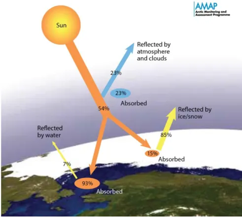
II.1.2. A positive feedback on sea ice melt: the decreasing albedo The albedo characterizes the “whiteness” of a surface; it is the ratio of radiation reflected from the surface to the incident radiation. The albedo is dimensionless and measured on a scale from zero (no reflection, black surface) to 1 (perfect reflection of a white surface). The seawater surface has then a lower albedo than the snow that is retained on the solid sea ice surface. This means that the incident
6
radiation is absorbed at a higher ratio when it arrives on the seawater than on the snow with the consequence that the seawater gets warmer than the snow surface. In the Arctic, as the global warming melts more ice, the global snow surface of the Earth and thus the Earth albedo both decrease, leading to a positive feedback where a bigger seawater surface absorbs the incident radiation and warms the Arctic Ocean (Figure II-1). This last figure is to be taken with care; the snow and ice albedo cannot be attributed to only one value as their albedo can easily differ according to their environment.
Figure II-1 : Albedo changes among marine environment (Arctic Monitoring and Assessment Programme, https://www.amap.no).
II.1.3. Atmospheric relevance of CO2 and N2O
Greenhouse gases such as carbon dioxide (CO2), methane (CH4) and nitrous oxide
(N2O) are recognised to be indirectly responsible for significant changes in the sea
ice cover in the polar regions, as these regions are sensitive to global warming. (IPCC, 2013). Representative concentration pathways (RCP) presented in the fifth assessment report of the IPCC (2013) propose four projections on global warming depending on GHG emissions for the 10 to 100 years to come. Across all RCPs, a
7
rise by 0.3 to 4.8 °C of the global mean temperature is projected by the late-21st century.
CO2 is a gas that is recognised to be the primary anthropogenic greenhouse gas
responsible for global warming. It is produced naturally or by human activities through fossil fuel or biomass combustion. The atmospheric concentration of CO2
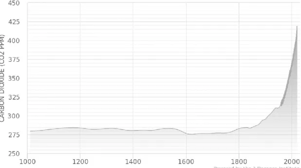
increased from about 280 ppm before the industrial era to more than 400 ppm (Figure II-2). The radiative effect of CO2 is also used as a reference for other
greenhouse gases as its global warming potential is set at a value equal to 1.
Figure II-2 : Changes in atmospheric CO2 abundance for the last 1019 years as
determined from air trapped in ice cores, firn air, and whole air samples. Data are from https://www.co2levels.org/#sources
N2O is a trace gas showing an electric dipole due to its asymmetry, providing
similar properties than CO2, i.e. their solubility and their diffusivity in water are
comparable (King et al., 1995; Wilhelm et al., 1977). With a lifetime of 114 years in the atmosphere (Ehhalt et al., 2001) and a global warming potential (GWP) up to 298 times that of CO2 (Forster et al., 2007), N2O is recognized as a potent
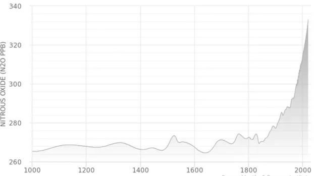
greenhouse gas naturally present in the atmosphere that exerts a significant influence on both climate and atmospheric chemistry. The atmospheric N2O
abundance determined from air trapped in ice cores, firn air and whole air samples shows a stable mixing ratio from 1000 to 1850 AD, between 265 to 275 ppb (or nmol
8
mol–1) while since 1850, N2O mixing ratio increases until today, where the monthly
mean value reached 332 ppb in January 2019 (Figure II-3).
Figure II-3: Changes in atmospheric N2O abundance for the last 1019 years as
determined from air trapped in ice cores, firn air, and whole air samples. Data are from http://www.n2olevels.org/#sources
The primary cause of this atmospheric increase in N2O is assumed to be the
agriculture and in particular, the use of synthetic fertilizers that enhance microbial activity and the animal waste management (Syakila and Kroeze, 2011). On the other hand, natural sources for N2O are significant and include terrestrial
soils by 61% and the ocean by 33% (Syakila and Kroeze, 2011). Due to its relatively long lifetime and thus its ability to reach the stratosphere, N2O is subject to
photochemical reactions in the stratosphere, a process that destroys the ozone so that N2O is the dominant ozone-depleting substance emitted in the 21st century
(Ravishankara et al., 2009).
II.1.4. The marine cycle of carbon and nitrogen
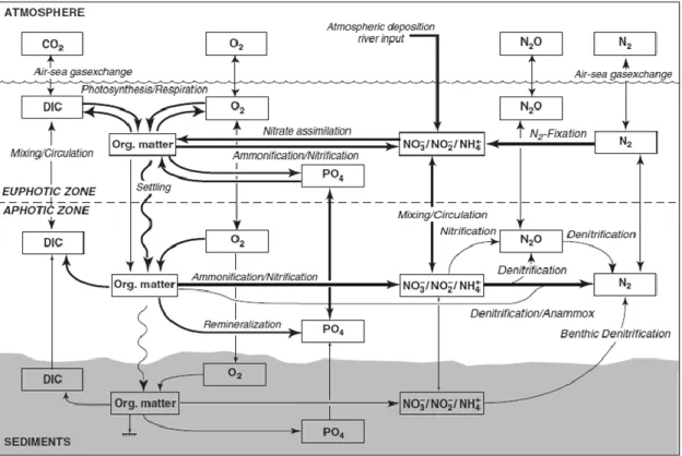
Nitrogen occupies a central position in the marine biogeochemistry, and has a significant influence on the carbon cycle (Figure II-4; Capone, 2008). The cycles start with carbon fixation during the photosynthesis in the upper ocean, a step that cannot take place without a supply of nitrogen-rich nutrients. This organic matter is respired or remineralized in the upper ocean, or exported and
9
remineralized in the ocean interior. From the deeper ocean, the matter that is returned to its inorganic form is transported back to the upper ocean by circulation and mixing (Capone, 2008). This biologically driven biogeochemical loop is fundamental for Earth’s climate, as it is one of the processes that determines the concentration of CO2 in the atmosphere. If this biogeochemical loop were
eliminated today, atmospheric CO2 would raise by more than 200 parts per million
(ppm) (Gruber and Sarmiento, 2002).
Figure II-4: Marine nitrogen cycle coupled with carbon, oxygen and phosphorus cycles. Figure from Capone (2008).
10
II.2. From a free-ice to an ice-covered seawater
II.2.1. Sea ice formation conditions and its resulting structure
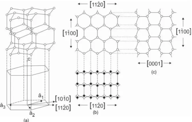
Sea ice forms from the freezing of seawater and its properties give indications on the seawater turbulence conditions during the formation of the first centimetres of sea ice. Sea ice crystallises in a specific system called Ih (Bragg, 1922; Weeks and Ackley, 1986), where H2O molecules are found to be tetrahedrally arranged within
themselves in a rotational symmetry of order 6 in the basal plane (c-axis in Figure II-5). The fasted growth occurs within the a-axis as it is an already build plane, while the orientation of the crystal is given by the c-axis, perpendicular to this basal plan (Figure II-5, Hobbs et al., 1974).
Figure II-5: Sea ice crystalline structure, where black points symbolise hydrogen atoms and white circles symbolise oxygen atoms (from Weeks and Ackley, 1986).
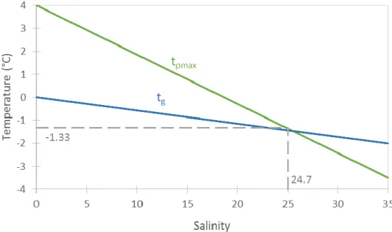
The addition of salt to the water lowers the temperature of maximum density (tρmax, Figure II-5). Once the salinity exceeds 24.7 (most Arctic surface water is
30-35), the water starts to freeze (by reaching tg) while getting denser. It may seem,
11
before freezing can begin at the surface, but in fact the Arctic Ocean is composed of layers of water with different properties, and at the base of the surface layer there is a big jump in density (known as a pycnocline), so convection only involves the surface layer down to that level (about 100-150 metres). This convection develops until the whole mixed layer (i.e. the water mass lying in between the surface and the pycnocline) reaches the freezing point, leading to the first crystal formation.
Figure II-6: Evolution of the maximum density temperature (tρmax) and the freezing
temperature (tg) with salinity (adapted from Weeks and Ackley, 1986).
This specific crystalline structure confers characteristic properties to sea ice: - a lower density than the one of liquid water, responsible for its buoyancy; - the limited incorporation of ions into the sea ice crystal lattice. In fact, during
sea ice growth, most of the ions originally present in seawater (Na+, K+, Ca+,
Mg+, Cl–, SO42–, CO32–) are either rejected back into the water column, or
trapped into liquid and gaseous inclusions into the sea ice matrix (Hobbs et al., 1974; Weeks and Ackley, 1986; Weeks and Gow, 1978);
- an advantageous growth rate within the basal plane, where molecules are preferentially added following a-axis (Hobbs et al., 1974).
12 II.2.2. Sea ice growth
Two processes limit crystal growth: the heat transfer and the transport of solutes through the liquid phase. During sea ice growth, it turns out that the heat transfer from the warm water mass to the cold interface is faster than the ions transport (rejected out the ice structure) in the opposite direction. A layer constitutionally supercooled then develops just below the growing ice (Weeks and Ackley, 1986) with a lower temperature than the freezing point. A minor disturbance of the supercooled ocean–sea ice interface triggers sea ice growth and results in thin vertical lamellar blades of ice crystals separated by films of brines (Weeks and Ackley, 1986). Heat and salts dissipations are local, non-linear inhomogeneous processes that favour growth where salts are concentrated (Nakawo and Sinha, 1981). The bottom end of the growing ice, called skeletal layer, is especially porous (around 30%) with a temperature just below the freezing point (Weeks and Ackley, 1986).
II.2.3. Sea ice texture
The analysis of the sea ice texture (i.e. its crystal morphology and fabric) gives indications on the way sea ice forms. The texture depends on the seawater conditions during sea ice formation (see growth conditions in Figure II-7) and the sea ice thickness (see depth and stratigraphy in Figure II-7). A typical succession of the different sea ice texture along with the first-year sea ice depth shows from top to bottom: granular ice, transition ice and columnar ice (Figure II-8).
Granular ice
The first unconsolidated crystals that form in turbulent waters are frazil ice crystals. Due to turbulence, these first crystals are small (1 to 10 mm long and less than 1 mm thick), randomly shaped, and randomly oriented. This particular texture in fully formed sea ice is referred to as granular ice (Figure II-8a).
13
Figure II-7: Synthesis of the different type of sea ice including the texture, the growth conditions among the time scale, and typical winter profiles of temperature and salinity for first-year sea ice (Petrich and Eicken, 2010).
Transition ice
A transition ice layer can be found between the granular and the columnar ice. The transition ice is composed of an intermediate texture with granular and columnar crystals (Figure II-8b).
Columnar ice
Once a thin layer of frazil covers ice and insulates the sea surface, congelation ice (or columnar ice) starts to form at the base of this frazil layer (Weeks and Ackley, 1986). Crystals of columnar ice have a specific prismatic, vertical, and elongated shape (Figure II-8c). This crystal orientation is due to a geometrical selection of advantageous vertical growth (Weeks and Gow, 1978).
14
Columnar ice may also start to grow at the sea surface provided relatively calm conditions.
Figure II-8: Pictures of three sea ice section from the Young Sound fjord (Greenland), on the 23/06/2014, observed with cross-polarized light. a) Top section (0 to 7 cm) of granular ice. b) Central section (33 to 40 cm) of transition ice. c) Bottom section (103 to 110 cm) of columnar ice.
Landfast ice and pack ice
Depending on the distance to the coast, two types of sea ice are commonly observed: the landfast ice and the pack ice. The landfast ice is formed close to the coasts, generally within quiet conditions, and remains fastened to the coast.
The presence of snow and seawater in the ice structure
Snow can contribute to the ice structure by the development of: (i) snow-ice, mostly at the beginning of the winter (e.g. Jeffries et al., 1997; Leppäranta, 1983) but also in spring and summer, or (ii) superimposed-ice that forms mostly at the beginning of the spring (e.g. Holt and Digby, 1985; Kawamura et al., 1997) at the ice surface. Accumulation of snow on thin sea ice in winter depresses sea ice surface below the sea level. Seawater then floods snow and freezes due to the low temperature of the snow. Frozen flooding seawater in the snow is referred as snow-ice. Snow-ice formation is observed in the Arctic Ocean and the Baltic Sea (Granskog et al., 2003) and the Okhotsk Sea (Nomura et al., 2010b). But it is more common in Antarctica where snow load is significant (Maksym and Jeffries, 2000).
In spring, snow is exposed to warmer temperatures and lower albedos (due to early melt of thinner snow patches), creating a pool of meltwater. As this meltwater
15
percolates downwards, it starts to refreeze when it reaches lower temperatures deep in the snow or at the snow-ice interface (Holt and Digby, 1985; Jeffries et al., 1994). This process is responsible for the formation of superimposed-ice, with a typical structure of hard fresh ice, creating an impermeable layer for gases. Superimposed-ice is also reported in Arctic regions like the Baltic and Beaufort seas (Eicken et al., 2004; Granskog et al., 2006) and over fast ice in Svalbard (Nicolaus et al., 2003).
The presence of microorganisms in the sea ice structure
Cold-adapted sea ice communities are present in the ice structure (Bowman et al., 1997; Junge et al., 2002) including microalgae, bacteria, micrograzers and virus that use different energy sources and comprise multiple trophic levels. Microorganisms are incorporated in the ice at the beginning of the ice growth (Garrison et al., 1989) and further develop in the sea ice that serves as a substrate (Horner et al., 1992) and protection against larger grazers (Krembs and Deming, 2008). Microalgae consist of mainly diatoms (about 90% in most studies), flagellates like prymnesiophytes, dinoflagellates, prasinophytes, chlorophytes among others. Smith et al., (1990) even present the ice (especially in the bottom few centimetres of the ice, closer from the nutrients reservoir) as one of the most favourable habitat for diatoms and other microalgae in the world’s oceans. However, the biomass of bacteria in a sea ice core can exceed algal biomass in winter (thanks to extracellular polymeric substances produced by bacteria and protecting them) and during algal bloom (Collins et al., 2008; Krembs et al., 2002, 2000). The organisms or bacteria groups that achieve the complete remineralization of organic compounds use different metabolic pathways and requiring diverse environmental conditions, such as aerobic and anaerobic micro-zones (Fripiat et al., 2014; Rysgaard and Glud, 2004).
16
II.3. The significant role of salts in sea ice
Sea ice salinity is a crucial tracer of physical processes and set several environmental conditions of importance for biogeochemistry. It is an indicator of sea ice biogeochemical properties since salts are concentrated in brine together with gases, nutrients and other impurities. Salinity and temperature play a critical role with respects to brine dynamics (described in section II.5.1), gas solubility and sea ice permeability (Hunke et al., 2011).
Salinity may be defined as absolute or practical salinity. Absolute salinity (SA, g
kg-1) is defined as the mass fraction of dissolved material in seawater and based on
the “density salinity” as presented in the TEOS-10 (IOC, 2010). Practical salinity (SP, dimensionless) is defined by the relation between the electrical conductivity of
a sample and the conductivity of a standard solution and is then converted in a practical salinity scale (IOC, 2010; UNESCO, 1978). These equations are valid for a range of salinity from 2 to 42 and for a temperature superior to –2°C.
II.3.1. What does salinity profiles state
Since around 80% of salts are rejected from sea ice during its formation, bulk sea ice salinity is lower than seawater salinity from which sea ice forms. After the initial salts rejection, salinity evolves across the seasons (Figure II-9, Malmgren, 1927; Nakawo and Sinha, 1981), and through years. Mean surface salinity of first-year ice is about 2 to 12, while that of multifirst-year ice approaches 0 (Weeks and Ackley, 1986).
17
Figure II-9: Evolution of sea ice salinity profiles with depth across the seasons (from
Malmgren, 1927). The C-shape salinity profile from October to March corresponds to the young first-year ice. Note that the reduction in surface salinity in June is due to meltwater flushing with the onset of summer melt.
II.3.2. Brine volume fraction and brine salinity relationships
As stated before, only a small amount of the salts is entrapped in the sea ice structure, within brine inclusions. The salinity and volume of these inclusions can be quantified in order to estimate the amount of impurities in the ice and its permeability to liquid and gases exchanges (see sections II.3.4 and II.4.2 respectively for more information).
Brine volume fraction
The brine volume fraction (BrV) is computed as a function of sea ice temperature and salinity according to the relationships proposed by Cox and Weeks (1983) and based on Assur (1958):
𝐵𝑟𝑉 =
𝑉𝑏𝑟 𝑉= (1 −
𝑉𝑎 𝑉)
𝜌𝑖𝑆𝑖 𝐹1(𝑇)− 𝜌𝑖𝑆𝑖𝐹2(𝑇) Equation II-1where V, Vbr and Va are the sea ice volume, the brine volume and the air volume in m3 respectively. The density of pure ice, ρi in kg m–3, is given by Equation II-2,
where T is in °C and the two functions F1(T) and F2(T) are given in Table II-1
following Equation II-3.
𝜌𝑖 = 917 − (1,403 × 10−4 𝑇) Equation II-2
18
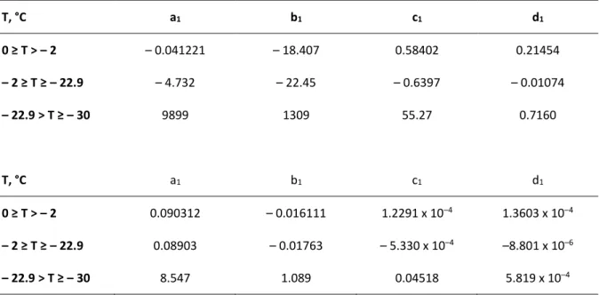
Table II-1: Coefficients for F1(T) and F2(T) for different temperature intervals by Cox and
Weeks (1983) and Leppäranta and Manninen (1988).
T, °C a1 b1 c1 d1 0 ≥ T > – 2 – 0.041221 – 18.407 0.58402 0.21454 – 2 ≥ T ≥ – 22.9 – 4.732 – 22.45 – 0.6397 – 0.01074 – 22.9 > T ≥ – 30 9899 1309 55.27 0.7160 T, °C a1 b1 c1 d1 0 ≥ T > – 2 0.090312 – 0.016111 1.2291 x 10⁻⁴ 1.3603 x 10⁻⁴ – 2 ≥ T ≥ – 22.9 0.08903 – 0.01763 – 5.330 x 10⁻⁴ –8.801 x 10⁻⁶ – 22.9 > T ≥ – 30 8.547 1.089 0.04518 5.819 x 10⁻⁴
In first-year ice, the air volume fraction Va/V can be neglected, because it is much smaller than Vb/V. It is not the case in multiyear ice, warm ice and snow-ice where Va/V should be taken into account in the Equation II-1 (Timco and Frederking, 1996). As a result, Vb/V can be considered as a good approximation of the sea ice porosity (Va+Vb)/V.
Brine salinity
The brine salinity (Sbr) is a function of sea ice temperature only. A change in
temperature will induce a change in the BrV by the freezing or melting of pure water in the brine inclusion (Hunke et al., 2011).
Several relationships between Sbr and T have been proposed.
Cox and Weeks (1986) suggest a relation derived from Assur (1958) where the coefficients used can be found in
Table II-2:
𝑆𝑏𝑟= 𝛼0+ 𝛼1𝑇 + 𝛼2𝑇2+ 𝛼
3𝑇3 Equation II-4
Notz (2005) suggests another relation based on (Assur, 1958), where T is the temperature in °C :
19
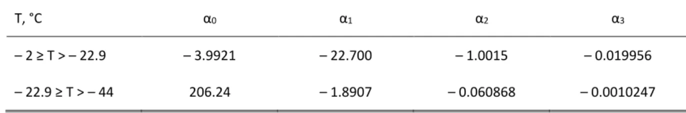
Table II-2: Coefficients used for Sbr in Equation II-4 (Cox and Weeks, 1986).
T, °C α0 α1 α2 α3
– 2 ≥ T > – 22.9 – 3.9921 – 22.700 – 1.0015 – 0.019956 – 22.9 ≥ T > – 44 206.24 – 1.8907 – 0.060868 – 0.0010247
Finally, Vancoppenolle et al. (2019) provide a new estimate of the Sbr based on an
agreement between observations and the Gibbs-Pitzer theory implemented in the FREZCHEM code (Marion et al., 1999). This gives the following equation:
𝑆𝑏𝑟= − 18.7 𝑇 − 0.519 𝑇2− 0.00535 𝑇3 Equation II-6
II.3.3. Brine concentration and dilution
In sea ice, gas concentration in brines strongly depends on ice temperature: when temperature decreases (i.e. during sea ice growth), the brine channels inclusions shrink in size by freezing pure water on the wall of the channels, concentrating salts, gases and other impurities in the brines – the so-called brine concentration process (e.g. Delille et al., 2014; Zhou et al., 2013). In opposite, when temperature increases, the melting of ice with the increase in the size of the brine inclusions dilutes their content – the so-called brine dilution process (Hunke et al., 2011; Notz and Worster, 2009).
II.3.4. Permeability threshold for liquid brine
Brine volume (denoted as BrV) provides information on how brine channels are connected together, and with the air above and the seawater below. Golden et al. (1998) suggested that sea ice permeability increases sharply for a BrV of 5%, a threshold that is well accepted. Below 5%, sea ice is considered as impermeable to brine transport, while above 5%, sea ice is considered as permeable, and as sea ice becomes permeable, air–ice gas exchange increases (Delille et al., 2014). The BrV threshold of 5% corresponds to an ice temperature of 5°C and a bulk ice salinity of 5.
20 II.3.5. Desalinisation processes
The desalinisation of sea ice encompasses the mechanisms by which brines – with its content in dissolved gas, nutrients and other impurities – are evacuated from the ice (Tsurikov, 1979). Sea ice can be approximate by two models; the boundary-layer that suggests a salt fractionation at the sea ice-seawater interface during sea ice formation, and the mushy-layer theory that suggests a continuum of salinity at the sea ice-seawater interface, and only considers two phases (ice and brine, no gas).
The best way to illustrate desalinisation processes is to compare the winter first-year sea ice salinity profiles with that of summer or multi-first-year sea ice (Figure II-9) to quantify the salt lost from sea ice growth to sea ice melt.
Several processes can explain the salinity variation within sea ice across the seasons, but only a few of them are relevant for this study (for more information, see Weeks, 2010, pp.156–170). Gravity drainage is the main process responsible for the rejection of dissolved gases to the ocean during ice growth (Moreau et al., 2014). Flushing by surface meltwater is commonly recognised to be the main desalinisation process during ice decay in the Arctic. Finally, brine rejection can develop upwards, at the sea ice-atmosphere interface; gas rejection potentially occurs in parallel with this salt rejection towards the ice surface, leading to significant air-sea ice gas fluxes during sea ice growth (Tison et al., 2017).
Initial brine rejection and incorporation
During the growth phase (see section II.2.2) and according to the boundary-layer theory, the growing sea ice rejects most of the salts at a freezing front (Burton et al., 1953; Cox and Weeks, 1975). Those salts then concentrate in the seawater at the interface of the freezing front, increasing the seawater salinity. Part of this saline seawater incorporates in the growing sea ice and forms the brine. The layer where the ice volume fraction varies from 0 to 30% is referred to as the skeletal layer (this paragraph is taken from Petrich and Eicken, 2010). According to the mushy-layer theory, the salinity in the skeletal layer is equal to the salinity of seawater at the ice interface, revealing that no salt is directly expelled at the advancing ice-seawater interface (Hunke et al., 2011; Notz and Worster, 2009).
21 Brine expulsion
This process occurs again during sea ice growth. Within the cooling sea ice, part of the liquid brine continues to freeze, forming pure ice. As pure ice is less dense than the brine, it will occupy a larger volume than the former brine and may create a fracture in the ice. This results in an upward or downward expulsion of brine (Bennington, 1963).
Gravity drainage
In wintertime, brine salinity generally decreases with temperature from the ice surface to its bottom. This salinity gradient creates, at the same time, an unstable density gradient that leads to brine convection where the ice is permeable. The convection of brine and its replacement with underlying seawater is referred to as gravity drainage through the mushy-layer theory (Notz and Worster, 2009; Worster and Wettlaufer, 1997).
Rayleigh number (Ra) introduced by Notz and Worster (2009) is a proxy for brine convection and is calculated using temperature, bulk ice salinity, derived brine salinity and brine volume fraction of the ice. However, as Ra depends on the gradient of brine salinity, the salts loss by drainage during ice core extraction, or the sampling resolution may lead to a different range of Ra values. However, there is no consensus on the critical value of Ra, leading to brine convection; Notz and Worster (2008) suggest that convection occurs above a Ra = 7, Notz and Worster (2009) then identify a critical Ra = 10, while some authors suggest to use the Ra in a qualitative way only, by comparing profiles to each other (Vancoppenolle et al., 2013; Zhou et al., 2013).
Flushing
During the melt season, the pressure of the snow meltwater creates a downward movement of brine (Eicken et al., 2002, 2004), reducing drastically the sea ice salinity.
Causes of a saline sea ice surface
The sea ice surface shows unique properties that may play a role in chemical processes occurring in the lower polar troposphere. For example, under intense
22
surface cooling, liquid water in brine freezes, increasing the dilating pure ice volume. This increase in volume can fracture the ice and therefore drive the expulsion of the remaining brine along the cracks to the ice surface (Bennington, 1963). This upward expulsion of brine (brine wicking) results in a high saline layer of brine skim (Untersteiner, 1968). Snow and frost flowers – a vapour-deposited ice crystals under strong relative humidity and temperature gradient at the ice–air interface (Barber et al., 2014) – can also influence the sea ice surface salinity by draining brine by capillarity, from the brine channels to the surface. Upward brine drainage by capillarity significantly increasing sea ice surface salinity, and thus the concentration in major ions, significantly (Domine et al., 2004; Douglas et al., 2012). Finally, flooding (see section II.2.3) may also add salts and impurities over the ice surface. Flooding then has the potential to impact the vertical salinity distribution in sea ice (Vancoppenolle et al., 2005, 2007). All the above mentioned physical processes are sources of salts and ions for the ice surface and create a suitable place for potential chemical reactions.
23 II.4. Gas bubbles within sea ice
This section describes the processes controlling gas bubbles content in sea ice.
II.4.1. Gas bubbles formation
Gas bubbles can be incorporated as air inclusions during sea ice formation. As brines are rejected at the sea ice–seawater boundary layer, their accumulation can be responsible for gas concentration that exceeds the solubility. Some studies (Killawee et al., 1998; Loose et al., 2009; Tison et al., 2002; Tsurikov, 1979) show that nucleation can occur in the boundary layer due to gas oversaturation, leading to the formation of gas bubbles that can be incorporated in sea ice. Moreover, observations show that turbulent conditions enhance gas incorporation in sea ice (Tison et al., 2002).
However, bubbles may also form within the ice during sea ice growth. Increase in gas concentration in brine due to the shrinking of brine inclusions (i.e. brine concentration, see section II.3.3) triggers the nucleation of bubbles (Tsurikov, 1979; Killawee et al., 1998; Tison et al., 2002; Light et al., 2003). The partitioning of gases between dissolved and gaseous forms in sea ice brine is a function of gas solubility, following Henry’s law:
𝐶𝑖,𝑏𝑟= 𝐾0× 𝑝𝑖 Equation II-7
where Ci,br (mol L–1) is the concentration of a gas dissolved in the solution, K0 (mol
L–1 atm–1) is the Henry’s constant, and pi (atm) is the partial pressure of the gas.
K0 is temperature and salinity dependant. During sea ice growth, the decrease in
brine temperature increases the solubility of the gases, while oppositely, the increase in brine salinity decreases the gas solubility. The net process is a decrease in gas solubility due to stronger salinity effect (see Figure 1b and 2a in Crabeck et al., 2019), leading eventually to an oversaturation. Bubbles then potentially form when the sum of the partial pressures of all the dissolved gases exceed the local hydrostatic pressure in brine (Crabeck et al., 2019; Delille et al., 2014; Geilfus et al., 2012a). In Crabeck et al. (2014a), bubbles started to form when the concentration exceeds 2.7 times the saturation with respect to the atmosphere. Crabeck et al. (2019) observed that the inner pressure in liquid brine is higher than
24
the atmospheric pressure during sea ice freezing, increasing gas solubility in discrete brine inclusions.
Besides the physical processes exposed above, biological activity may also contribute to the presence of gas bubbles in sea ice (e.g. Delille et al., 2007; Tsurikov, 1979; Zhou et al., 2014a).
II.4.2. Total gas content
The air volume fraction (Va) of sea ice can be determined from bulk temperature, salinity, and density measurements (Cox and Weeks, 1983). Other methods use imaging to describe and quantify air inclusions within sea ice. For instance, Light et al. (2003) used transmitted light with a relatively poor resolution. A new method developed in Crabeck et al. (2016) involves computed tomography with X-ray imaging and gives a much higher resolution. In this last study, total gas content was estimated for the full length of some ice cores with a high vertical resolution (see the red curve in Figure II-10 where Va range between 0 and 20%) in parallel with the sea ice texture (thin sections in Figure II-10). Such approach confirmed that the permeability of granular ice is lower than the one of the columnar ice as previously suggested in other studies (Golden et al., 1998). Finally, Crabeck et al. (2016) suggested that sea ice structure and gas solubility control the air volume fraction contained in sea ice.
II.4.3. Permeability thresholds for gas bubbles
The presence of gas bubbles in a gas permeable sea ice promotes gas exchange with the atmosphere. Bubbles migrate upwards when the brine network is connected, which is assumed to happen above a given brine fraction threshold, reported as higher for gases (BrV = 7 to 10%, in Moreau et al., 2014; Zhou et al., 2013), compared to liquids (BrV = 5%, see section II.3.4). This higher threshold for gases was ascribed to ice tortuosity that hampers bubble movement in the brine network (Zhou et al., 2013).
25
Figure II-10: Sea ice thin sections and air volume fraction (red curve) for 14, 16 and 25 of January. The zero depth is fixed at the boundary between granular and columnar ice
26 II.5. Gas transport in sea ice
Gases can be found in sea ice in either solid contribution (i.e. salt precipitates, like ikaite), dissolved (i.e. brines) or gaseous phases (i.e. bubbles in liquid brines or within the ice matrix, e.g. O2, Ar, CH4 in Crabeck et al., 2014a; Moreau et al., 2014
and Zhou et al., 2013). The presence of gases in sea ice under one of these three phases will have a totally different impact on their further transport (Crabeck et al., 2019): solid phase is likely to be trapped in sea ice (Delille et al., 2014), dissolved gases in brine will follow the brine dynamics, while gas bubbles will be subject to buoyancy and upward migration (Crabeck et al., 2016), potentially driving air–ice gas exchanges.
II.5.1. Brine and bubbles dynamics from sea ice growth to sea ice decay
Zhou et al. (2013) suggested that bubbles and brine dynamics from sea ice growth to its decay can be divided into three stages (Figure II-11).
(i) During the cold stage, an initial entrapment of gas first occurs with sea ice formation, followed by bubble nucleation during sea ice growth. This stage is associated with low permeability in the ice, which limits gas transport to sea ice bottom layer convection and molecular diffusion. (ii) During the transition stage, freshwater from internal melting increases
the brine volume and lowers its salinity. Three factors promote bubble nucleation: changes in temperature (T) and salinity (S), the presence of hydrophobic impurities, and full-depth convection. Bubbles can then migrate upwards in permeable layers due to their buoyancy, while the liquid phase (including dissolved gases) moves with brine convection. Gas diffusion (Crabeck et al., 2014a; Loose et al., 2011) and the formation of superimposed ice may also control gas content in permeable sea ice. (iii) The warm stage corresponds to brine stratification as a result of prior
convection or ice melting that reduces brine density anomalies and cut convection (despite sea ice permeability). During this phase, bubbles are less abundant since the source of bubble formation dies out, as internal
27
melting decreases gas concentration in brine below the saturation threshold.
Figure II-11: A schematic view of the three stages of brine dynamics described in Zhou et al. (2013). More information in section II.5.1.
II.5.2. Gas diffusion
In the absence of brine convection, gases are transported in the ice by diffusion. In the literature, two paths for gas diffusion have been brought out:
The diffusive path of dissolved gases in brines: these gases diffuse in brines following the concentration gradient (Crabeck et al., 2014a; Loose et al., 2011).
The diffusive path for gaseous phase: Gosink et al. (1976) and Loose et al. (2011) suggest that gas bubbles can migrate along the grain boundaries within the ice matrix.
28
II.6. CO2 dynamics within the ice and at the interfaces
II.6.1. Overview of the carbonate chemistry system
In seawater and brines, the major species that compose the carbonate system are CO2, H2CO3, HCO3– and CO32–. Carbonate species are in equilibrium according to
the dissociation constants of the carbonate system (K1 and K2, the first and the
second dissociation constants, see Figure II-12), while CO2 concentration is in
equilibrium with atmospheric CO2 according to Henry’s law, Ko being the
solubility coefficient of CO2 in seawater. These constants are temperature, salinity
and pressure dependants (Zeebe and Wolf-Gladrow, 2001). To date, studies of CO2
in sea ice has been carried out with constants developed for seawater at positive temperature and within the range of salinity commonly observed in the ocean. It was assumed that the constants are valid at sub-zero temperature and high salinities. It was suggested that the best set of constants is Goyet and Poisson (1989; Brown et al., 2014). A more obvious approach is computation of carbonate system using Pitzer type parametrisation (Marion, 2001).
𝐂𝐎𝟐(𝐠) 𝐀𝐭𝐦𝐨𝐬𝐩𝐡𝐞𝐫𝐞
𝐂𝐎𝟐 (𝐚𝐪) + 𝐇𝟐𝐎 ↔ 𝐇𝟐𝐂𝐎𝟑 ↔ 𝐇𝐂𝐎𝐊𝟏 𝟑−+ 𝐇+ 𝐊𝟐
↔ 𝐂𝐎𝟑𝟐−+ 𝟐𝐇+
Ocean
Figure II-12: Simplified overview of the carbonate system in the ocean in contact with the atmosphere and in standard conditions (adapted from Zeebe and Wolf-Gladrow, 2001).
The sum of the dissolved C-species is named DIC, in µmol kg–1, for dissolved
inorganic carbon:
𝐷𝐼𝐶 = [𝐶𝑂2] + [𝐻𝐶𝑂3−] + [𝐶𝑂32−] Equation II-8
Speciation of the carbonate system can be computed using a few measurable parameters. Among them, total alkalinity (TA) measures the equilibrium of weak acids (pK < 4.5 at 25°C and zero ionic strength) with their conjugate bases:
𝑇𝐴 = [𝐻𝐶𝑂3−] + 2[𝐶𝑂
32−] + [𝐵(𝑂𝐻)4−] + [𝑂𝐻−] + [𝐻𝑃𝑂42−] + 2[𝑃𝑂43−] + [𝐻3𝑆𝑖𝑂4−] +
[𝑁𝐻3] + [𝐻𝑆−] − [𝐻+] − [𝐻𝑆𝑂4−] − [𝐻𝐹] − [𝐻3𝑃𝑂4] Equation II-9 K0