HAL Id: lirmm-00511830
https://hal-lirmm.ccsd.cnrs.fr/lirmm-00511830
Submitted on 26 Aug 2010
HAL is a multi-disciplinary open access
archive for the deposit and dissemination of sci-entific research documents, whether they are pub-lished or not. The documents may come from teaching and research institutions in France or abroad, or from public or private research centers.
L’archive ouverte pluridisciplinaire HAL, est destinée au dépôt et à la diffusion de documents scientifiques de niveau recherche, publiés ou non, émanant des établissements d’enseignement et de recherche français ou étrangers, des laboratoires publics ou privés.
Estimating maximum likelihood phylogenies with
PhyML
Stéphane Guindon, Frédéric Delsuc, Jean-François Dufayard, Olivier Gascuel
To cite this version:
Stéphane Guindon, Frédéric Delsuc, Jean-François Dufayard, Olivier Gascuel. Estimating maxi-mum likelihood phylogenies with PhyML. David Posada. Bioinformatics for DNA Sequence Analysis, Springer Protocols, pp.113-137, 2009, Methods in Molecular Biology, �10.1007/978-1-59745-251-9_6�. �lirmm-00511830�
Estimating maximum likelihood phylogenies with PhyML
St´ephane Guindon1,3
Fr´ed´eric Delsuc2
Jean-Fran¸cois Dufayard1
Olivier Gascuel1
1: Laboratoire d’Informatique, de Robotique et de Micro´electronique de Montpellier (LIRMM). UMR 5506-CNRS, Universit´e Montpellier II, Montpellier, France.
2: Institut des Sciences de l’Evolution de Montpellier (ISEM), UMR 5554-CNRS, Univer-sit´e Montpellier II, Montpellier, France.
3: Department of Statistics - The University of Auckland. Auckland, New Zealand.
Keywords: DNA and protein sequences, molecular evolution, sequence comparisons, phy-logenetics, statistics, maximum likelihood, Markov models, algorithms, software, PhyML.
Running title: Reconstruction of phylogenies using PhyML.
Corresponding author: Stephane Guindon Department of Statistics The University of Auckland Private Bag 92019
Auckland, New Zealand
Phone: +649 3737599 x82755 Fax: +649 3737018
Abstract
Our understanding of the origins, the functions and/or the structures of biological sequences strongly depends on our ability to decipher the mechanisms of molecular evo-lution. These complex processes can be described through the comparison of homologous sequences in a phylogenetic framework. Moreover, phylogenetic inference provides sound statistical tools to exhibit the main features of molecular evolution from the analysis of actual sequences. This chapter focuses on phylogenetic tree estimation under the maxi-mum likelihood (ML) principle. Phylogenies inferred under this probabilistic criterion are usually reliable and important biological hypotheses can be tested through the compari-son of different models. Estimating ML phylogenies is computationally demanding though and careful examination of the results is warranted. This chapter focuses on PhyML, a software that implements recent ML phylogenetic methods and algorithms. We illustrate the strengths and pitfalls of this program through the analysis of a real data set. PhyML v3.0 is available from http://atgc.lirmm.fr/phyml
1
Introduction.
In statistics, models are mathematical objects designed to approximate the processes that generated the data at hand. These models can be more or less complex, depending on the type of data and the available knowledge on the process that generated them. Each model has parameters which values need to be estimated from the data. Least-squares, maximum a posteriori estimation (MAP) or maximum likelihood (ML) are the main sta-tistical frameworks suitable for this task. The least-squares criterion has been widely used in phylogenetics in order to build trees from matrices of pairwise distances between se-quences. The last two criteria, ML and MAP, both rely on the probability that the data were generated according to the selected model. This conditional probability is the likeli-hood of the model. The next section gives a short description of the type of models that are used for phylogenetic inference.
1.1 Mathematical description of sequence evolution.
In molecular evolution, we commonly assume that homologous sequences evolve along a bifurcating tree or phylogeny. The topology of this tree describes the different clades or groups of taxa. The tree topology is generally considered to be the most important param-eter of the whole phylogenetic model. The second paramparam-eter is the set of branch lengths on a given topology. The length of each branch on this topology represents an amount of evolution which corresponds to an expected number of nucleotide, codon or amino-acid substitutions. The last component of the model is a mathematical description of the pro-cess that generates substitutions during the course of evolution. Several assumptions are made about this process. We first consider that the sites of the alignment, i.e., its columns, evolve independently (see Note 1) and under the same phylogeny. We also assume that the substitution process is the same at the different sites of the alignment. This process is modelled with Markov chains. The two main components of a Markov model of substitu-tion are (1) a symmetrical matrix that describes the relative speed at which the different substitution events occur (e.g., transition and transversion rates are generally distinct), and (2) the frequencies of the different states to be considered (i.e., nucleotides, codons or amino-acids). The symmetrical matrix is often referred to as the exchangeability ma-trix. If combined with the vector of state frequencies, the resulting matrix corresponds to the generator of the Markov process and the vector of state frequencies is the stationary
distribution.
1.2 A difficult optimisation problem.
ML tree estimation consists of finding the phylogenetic model, i.e., the tree topology, branch lengths and parameters of the Markov model of substitution, that maximises the likelihood. Calculating the likelihood of a given phylogenetic model can be done efficiently using Felsenstein’s pruning algorithm (1). Unfortunately, finding the ML model is a difficult problem. The difficulty mostly comes from the very nature of the model itself. Indeed, while branch lengths and parameters of the substitution model are continuous variables, the tree topology is a discrete parameter. Hence, it is not surprising that, for most data sets, the likelihood function defines a rugged landscape with multiple peaks (see (2) however). Searching for the ML phylogenetic model in such conditions therefore rely on sophisticated optimisation methods, which combine both discrete and continuous optimisation procedures.
These methods are heuristics. As opposed to exact algorithms, heuristics do not guar-antee to find the best (i.e., ML) solution. Despite this, simulation studies (3, 4) suggest that the heuristics designed for phylogenetic estimation perform well overall. The most ef-ficient methods are those that provide the best trade-off between their ability to maximise the likelihood function and the time spent to achieve this. Several methods/programs use deterministic approaches: given an initial non-optimal solution, the heuristic always follows the same path of intermediate solutions to reach the estimated ML one. As a con-sequence, given a particular input (i.e., data and model settings), these methods always produce the same output (i.e., the estimated ML phylogenetic model). Other approaches implement non-deterministic heuristics. These methods do not always follow the same path of intermediate solutions to reach the estimated ML tree. Hence, the same input potentially leads to distinct outputs (see Note 2).
1.3 Searching through the space of tree topologies.
Another important distinction between tree building methods lies in the type of operations (or moves) that are used to explore the space of tree topologies. The three principal moves are: nearest neighbour interchange (NNI), subtree pruning and regrafting (SPR) and tree bisection and reconnection (TBR) (see (4)). Each of these moves permits an exhaustive exploration of the space of tree topologies. However, the neighbourhood of trees defined
by applying TBR moves to any given topology is much wider than the neighbourhood defined by SPR moves, which is itself larger than the neighbourhood defined by NNI moves. Therefore, TBRs are more efficient than SPRs or NNIs in jumping across very distinct tree topologies in just one step. The same also holds for SPR vs. NNI moves. These differences result in various abilities to escape local maxima of the likelihood function. Consider a suboptimal peak of the likelihood surface and the tree topology found at this peak. Every potential NNI move will only allow to reach similar topologies. Therefore, such moves will sometimes fail to reach a higher peak of the likelihood surface. Hence, SPR operations are more efficient than NNIs in finding the highest peaks of the likelihood surface and TBR moves are more efficient than SPR ones. However, the large neighbourhood of trees defined by TBR compared to SPR or NNI also generally implies greater run times. Basically, many non-optimal solutions are evaluated when using TBR moves as compared to SPRs or NNIs. Hence, the best methods with respect to likelihood maximisation also tend to be the slowest ones.
1.4 PhyML v3.0: new features.
PhyML (5) is a software that estimates ML phylogenies from alignments of nucleotide or amino acid sequences. It provides a wide range of options that were designed to facilitate standard phylogenetic analyses. This chapter focuses on PhyML v3.0. This version of the program provides two important advances compared to the previous releases. Indeed, PhyML v3.0 now proposes three different options to search across the space of phylogenetic tree topologies. It also implements a new method that evaluates branch supports. These new options are presented below.
1.5 Escaping local maxima.
PhyML originally relies on a deterministic heuristic based on NNI moves. Traditional greedy approaches first evaluate the gain of likelihood brought by every possible NNI ap-plied to the current topology. Only the best move is then used to improve the phylogeny at each step of the tree building process. Hence, most of the calculations evaluate moves that will not be used subsequently. To avoid such waste of potentially useful information, PhyML applies several ‘good’ NNI moves simultaneously. Moreover, these local and si-multaneous changes of the tree topology are accompanied by adjustments of every branch length in the phylogeny (see Note 3). Hence, most of the calculations that are performed
during one step of the algorithm are actually used to improve the tree. This is what makes PhyML faster than popular algorithms such a fastDNAml (6), and simulation results (5) demonstrated the accuracy of this approach. PhyML also outperforms the standard NNI-based greedy searching algorithms in terms of maximisation of the likelihood function. However, the analysis of real data and the comparison with SPR-based algorithms shows that PhyML occasionally gets trapped in local maxima. This shortcoming is more and more obvious as the number of sequences to analyse gets large (i.e., > 50-100). Hence, while the phylogenetic models estimated with PhyML are generally good in terms of like-lihoods, models with greater likelihoods can often be found.
This is the reason why the release 3.0 of PhyML proposes new SPR-based tree search-ing options. The methods implemented in PhyML v3.0 are inspired by Hordijk and Gas-cuel (7) work on the topic. Their approach essentially relies on using a fast distance-based method to filter out SPR moves that do not increase the likelihood of the current phy-logenetic model. Hence, the likelihood function is only evaluated for the most promising moves. This strategy proves to be efficient in finding trees with high likelihoods. While the computational burden involved with SPRs is heavier than with simultaneous NNIs, this new approach is clearly less prone to be stuck in local maxima of the likelihood function (see Note 4).
PhyML 3.0 also proposes an intermediate option that includes both NNIs and SPRs. Simultaneous NNIs are first applied following the original algorithm, until no additional improvement is found. A single round of SPR moves are then tested: each subtree is pruned, regrafted, filtered and only the most promising moves are actually evaluated. If one or more SPR moves increase the likelihood, the best one is applied to the current tree. A new round of simultaneous NNIs then starts off after this step. Simultaneous NNIs and SPRs therefore alternate until a maximum of the likelihood function is reached. This approach is generally faster than the SPR-only one but slower than the NNI-based heuristic. Also, while this strategy performs better than the NNI-only one in optimising the likelihood function, the SPR-only search often outperforms this mixed approach.
1.6 Fast tests for branch support.
PhyML v3.0 also provides users with a fast approximate likelihood ratio test (aLRT) for branches (8), which proves to be a good alternative to the (time-consuming) bootstrap analysis. The aLRT is closely related to the conventional LRT, with the null hypothesis
corresponding to the assumption that the tested branch has length 0. Standard LRT uses
the test statistics 2(L1− L0), where L1 is the log-likelihood of the current tree, and L0 the
log-likelihood of the same tree, but with the branch of interest being collapsed. The aLRT
approximates this test statistics in a slightly conservative but practical way as 2(L1− L2),
where L2 corresponds to the second best NNI configuration around the branch of interest.
Such test is fast because the log-likelihood value L2 is computed by optimising only over
the branch of interest and the four adjacent branches, while other parameters are fixed at their optimal values corresponding to the best ML tree. Three branch supports computed from this aLRT statistics are available in PhyML v3.0: (1) the parametric branch support,
computed from the χ2
distribution (as usual with the LRT); (2) a non-parametric branch support based on a Shimodaira-Hasegawa-like procedure (9); (3) a combination of these two supports, that is, the minimum value of both. The default is to use SH-like branch supports.
The rational behind the aLRT clearly differs from non-parametric bootstrap, as de-tailed in (8). Basically, while aLRT values are derived from testing hypotheses, the bootstrap proportion is a repeatability measure; when the bootstrap proportion of a given clade is high, we are quite confident that this clade would be inferred again if another original data sample was available and analysed by the same tree-building method (which does not mean that the clade exists in the true tree). Also, computing aLRT values is much faster than getting bootstrap supports, as PhyML is run just once, while bootstrap requires launching PhyML 100 to 1,000 times. In fact, computing aLRT branch supports has a negligible computational cost in comparison with tree building. Note however that SH-like branch supports are non-parametric, just as are the bootstrap proportions. In fact, they often provide similar results as the bootstrap, pointing out the same poorly supported branches of the phylogeny, as illustrated in Fig. 1.
The aLRT assesses that the branch being studied provides a significant gain in like-lihood, in comparison with the null hypothesis that involves collapsing that branch but leaving the rest of the tree topology identical. Thus, the aLRT does not account for other possible topologies that would be highly likely but quite different from the current topol-ogy. This implies that the aLRT performs well when the data contains a clear phylogenetic signal, but not as well in the opposite case, where it tends to give a (too) local view on
the branch of interest and be liberal. Note also that parametric χ2
branch supports are based on the assumption that the evolutionary model used to infer the trees is the correct
one. In that respect, the aLRT parametric interpretation is close to Bayesian posteriors. As the later, the resulting test is sometimes excessively liberal due to violations of the parametric assumptions.
Let us now focus on the practical aspects that go with ML phylogenetic model estima-tion using PhyML v3.0. The next secestima-tion presents the inputs and outputs of the program, the different options and how to use them.
2
Program usage.
PhyML v3.0 has two different user interfaces. The default is to use the PHYLIP-like text interface (Fig. 2) by simply typing ‘phyml’ in a command-line window or by clicking on the PhyML icon (see Note 5). After entering the name of the input sequence file, the user goes through a list of sub-menus that allow her/him to set up the analysis. There are currently four distinct sub-menus:
1. Input Data: specify whether the input file contains amino acid or nucleotide se-quences. What is the sequence format (see Section 2.1) and how many data sets should be analysed.
2. Substitution Model: selection of the Markov model of substitution (see Section 2.2). 3. Tree Searching: selection of the tree topology searching algorithm (see Section 2.4). 4. Branch Support: selection of the method that is used to measure branch support
(see Section 2.3).
‘+’ and ‘-’ keys are used to move forward and backward in the sub-menu list. Once the model parameters have been defined, typing ‘Y’ (or ‘y’) launches the calculations. The meaning of some options may not be obvious to users that are not familiar with phylogenetics. In such situation, we strongly recommend to use the default options. As long as the format of the input sequence file is correctly specified (sub-menu Input data), the safest option for non-expert users is to use the default settings.
The alternative to the PHYLIP-like interface is the command line. Users that do not need to modify the default parameters can launch the program with the ‘phyml -i your input sequence file name’ command. The list of all command line arguments and how to use them is given in the ‘Help’ section which is displayed after entering the
‘phyml help’ command. Command lines are specially handy for launching PhyML v3.0 in batch mode. Note however that some options are only available through the PHYLIP-like interface. Hence, options that are not listed in the ‘Help’ section may be accessible through the interactive text interface.
2.1 Inputs / outputs.
PhyML reads data from standard text files, without the need for any particular file name extension. Alignments of DNA or protein sequences must be in PHYLIP sequential or interleaved format (see Fig. 3a). The first line of the input file contains the number of species and the number of characters, in free format, separated by blanks. One slight difference with PHYLIP format concerns sequence name lengths. While PHYLIP format limits this length to ten characters, PhyML can read up to hundred character long sequence names. Blanks and the symbols “(),:” are not allowed within sequence names because the NEWICK tree format makes special use of these symbols (Fig. 3b).
Another slight difference with PHYLIP format is that actual sequences must be sep-arated from their names by at least one blank character. These sequences must not be
longer than 106
amino acid or nucleotide characters and a given data set can have up to
4×10³
of them. However, the size of the largest data set PhyML v3.0 can process depends on the amount of physical memory available. To avoid overflows, PhyML v3.0 pauses when the estimated amount of memory that needs to be allocated exceeds 250Mb. The user can then decide whether she/he wants to continue or cancel the analysis (see Note 6).
An input sequence file may also display more than a single data set. Each of these data sets must be in PHYLIP format and two successive alignments must be separated by an empty line. Processing multiple data sets requires to toggle the ‘M’ option in the Input Data sub-menu or use the ‘-n’ command line option and enter the number of data sets to analyse. The multiple data set option can be used to process re-sampled data that were generated using a non-parametric procedure such as cross-validation or jackknife (a bootstrap option is already included in PhyML). This option is also useful in multiple gene studies, even if fitting the same substitution model to all data sets may not be suitable.
Gaps correspond to the ‘-’ symbol. They are systematically treated as unknown char-acters “on the grounds that we don’t know what would be there if something were there” (J. Felsenstein, PHYLIP main documentation). The likelihood at these sites is summed over all the possible states (i.e., nucleotides or amino acids) that could actually be observed
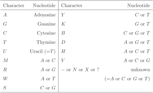
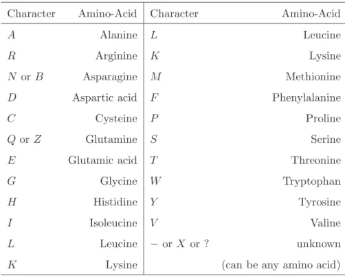
at these particular positions. Note however that columns of the alignment that display only gaps or unknown characters are simply discarded because they do not carry any phy-logenetic information (they are equally well explained by any model). PhyML v3.0 also handles ambiguous characters such as R for A or G (purines) and Y for C or T (pyrim-idines). Tables 1 and 2 give the list of valid characters/symbols and the corresponding nucleotides or amino acids.
PhyML v3.0 can read one or several phylogenetic trees from an input file. This option is accessible through the Tree Searching sub menu or the ‘-u’ argument from the command line. Input trees are generally used as initial ML estimates to be subsequently adjusted by the tree searching algorithm (see Section 2.4). This option is also helpful when one wants to evaluate the likelihood on a particular set of (possibly competing) phylogenetic trees. Trees should be in standard NEWICK format (Fig. 3b). They can be either rooted or unrooted and multifurcations are allowed. Taxa names must, of course, match the corresponding sequence names.
Single or multiple sequence data sets may be used in combination with single or multiple
input trees. When the number of data sets is one (nD = 1) and there is only one input
tree (nT = 1), then this tree is simply used as input for the single data set analysis. When
nD = 1 and nT > 1, each input tree is used successively for the analysis of the single
alignment. If nD >1 and nT = 1, the same input tree is used for the analysis of each data
set. The last combination is nD > 1 and nT > 1. In this situation, the i-th tree in the
input tree file is used to analyse the i-th data set. Hence, nD and nT must be equal here.
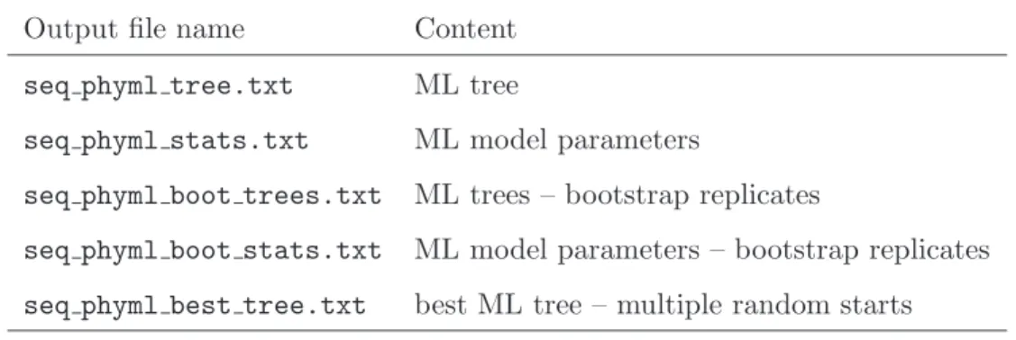
Table 3 presents the list of files resulting from a PhyML v3.0 analysis. Basically, each output file name can be divided into three parts. The first part is the sequence file name, the second part corresponds to the extension ‘ phyml ’ and the third part is related to the file content. When launched with the default options, PhyML v3.0 only creates two files: the tree file and the model parameter file. The estimated ML tree is in standard NEWICK format (Fig. 3b). The model parameters file, or statistics file, displays the ML estimates of the substitution model parameters, the likelihood of the ML phylogenetic model, and other important information concerning the settings of the analysis (e.g., type of data, name of the substitution model, starting tree (see Section 2.4), etc.). Two additional output files are created if bootstrap supports were evaluated. These files simply contain the ML trees and the substitution model parameters estimated from each bootstrap replicate. Such information can be used to estimate sampling errors
around each parameter of the phylogenetic model. The best ML tree file is only created when the estimation of the phylogeny resulted from multiple random starting trees. It contains the tree with the highest likelihood that was found among all the trees estimated during the analysis (see Section 2.4).
2.2 Substitution models.
PhyML implements a wide range of substitution models: JC69 (10), K80 (11), F81 (1), F84 (12), HKY85 (13), TN93 (14) GTR (15, 16) and CUSTOM for nucleotides ; WAG (17), Dayhoff (18), JTT (19), Blosum62 (20), mtREV (21), rtREV (22), cpREV (23), DCMut (24), VT (25) and mtMAM (26) for amino acids. Nucleotide equilibrium frequencies are estimated by counting the occurrence of A, C, G and T s in the data (see Note 7).
These frequencies can also be adjusted in order to maximise the likelihood of the phy-logenetic model (Substitution Model sub-menu, option ‘F’ ; command line argument : ‘-f e’) or deduced from the actual sequences. Amino acid equilibrium frequencies are either deduced from the actual sequences (Substitution Model sub-menu, option ‘F’ ; command line argument : ‘-f e’) or given by the substitution models themselves (default option).
The CUSTOM option provides the most flexible way to specify the nucleotide substi-tution model. The model is defined by a string made of six digits. The default string is ‘000000’, which means that the six relative rates of nucleotide changes: A ↔ C, A ↔ G, A ↔ T , C ↔ G, C ↔ T and G ↔ T , are equal. The string ‘010010’ indicates that the rates A ↔ G and C ↔ T are equal and distinct from A ↔ C = A ↔ T = C ↔ G = G ↔ T . This model corresponds to HKY85 (default) or K80 if the nucleotide frequencies are all set to 0.25. ‘010020’ and ‘012345’ correspond to TN93 and GTR models respectively. The digit string therefore defines groups of relative substitution rates. The initial rate within each group is set to 1.0, which corresponds to F81 (JC69 if the base frequencies are equal). Users also have the opportunity to define their own initial rate values (this option is only available through the PHYLIP-like interface). These rates are then optimised afterwards (option ‘O’) or fixed to their initial values. The CUSTOM option can be used to implement all substitution models that are special cases of GTR.
PhyML v3.0 also implements Ziheng Yang’s discrete gamma model (27) to describe the variability of substitution rates across nucleotide or amino acids positions. Users can specify the number of substitution rate categories (Substitution Model sub-menu option
‘C’ or ‘-c’ argument from the command line) and choose to estimate the gamma shape parameter from the data or fix its value a priori (option ‘A’ or ‘-a’). The program also handles invariable sites (option ‘V’ or ‘-v’). Here again, the value of this parameter can be estimated in the ML framework or fixed a priori by the user (see Note 8)
2.3 Branch support.
PhyML v3.0 proposes two main options to assess the support of the data for non-terminal branches in the phylogeny. The most popular approach relies on non-parametric bootstrap. This option is available through the PHYLIP-like interface (Branch Support sub-menu) or the ‘-b’ argument from the command line. Users only have to specify the number of replicates that will be generated to work out the bootstrap values. The ML output tree (see Section 2.1) will then display both branch lengths and bootstrap values. It is very important to keep in mind that bootstrap values are displayed on the ML tree estimated from the original data set. There is no consensus tree reconstruction involved here. Note however that PhyML also outputs every tree estimated from the re-sampled data sets. These trees can then be used to build a consensus tree, using the program CONSENSE from the PHYLIP package for instance. However, there is no guarantee that this consensus tree is also the ML tree (but both generally have similar topologies).
PhyML v3.0 also implements the approximate likelihood-ratio tests (aLRT) described in Section 1.6. Just like bootstrap support, aLRT options are available from the Branch Support sub-menu in the PHYLIP-like interface. The ‘A’ key is used to choose among four distinct options as aLRT supports can be assessed through different tests. The default
is to use SH-like branch supports. It is also possible to test aLRT values against a χ2
distribution or to use a combination of these last two options. Expert users also have the opportunity to retrieve the aLRT values themselves in order to examine the differences of likelihood among competing topologies. These four options are also available using the ‘-b’ argument from the command line as explained in the ‘Help’ section.
2.4 Tree searching algorithms.
PhyML v3.0 implements three heuristics to explore the space of tree topologies (see Section 2). All methods take as input a starting tree that will be improved subsequently. The default is to let PhyML v3.0 build this starting tree using BioNJ (28). However, users can also give their own input tree(s) in NEWICK format (see Section 2.1). Under the
default settings, the starting tree is improved using simultaneous NNIs. PhyML v3.0 also proposes NNI+SPR and full-SPR heuristics that both search more thoroughly the space of tree topologies. Simultaneous NNIs, NNI+SPR and full-SPR options are available from the Tree Searching sub-menu or the ‘-s’ argument from the command line.
Full-SPR searches can also be combined with multiple random starting trees (Tree Searching sub-menu, options ‘S’ and ‘R’). Multiple random starting solutions are useful to evaluate the difficulty of the optimisation problem given the data at hand. Indeed, if the estimated solution (the ML phylogenetic model in our case) strongly depends on the value that is used to initiate the optimisation process (the starting tree), then the function to optimise is probably not smooth and local optima are likely to be commonplace. Hence, multiple random starting trees provide a diagnosis tool to evaluate the smoothness of the likelihood surface and the robustness of the inferred tree. The default is to use five random starting trees. Five ML phylogenetic models are then estimated and the best phylogenetic tree (i.e., the tree with the highest likelihood) is printed in the ‘ phyml best tree.txt’ file (Table 3). When all these trees are identical, this tree is likely to be the ML solution.
2.5 Recommendations on program usage.
From the user perspective, the choice of the tree searching algorithm among those provided by PhyML v3.0 is probably the toughest one. The fastest option relies on local and simultaneous modifications of the phylogeny using NNI moves. More thorough explorations of the space of topologies are also available through the NNI+SPR and full-SPR options. As these two classes of tree topology moves involve different amounts of computation, it is important to determine which option is the most suitable for the type of data set or analysis one wants to perform. Below is a list of recommendations for typical phylogenetic analyses.
1. Single data set, unlimited computing time. The best option here is probably to use a full-SPR search. If the focus is on estimating the relationships between species (see Section 3), it is a good idea to use more than one starting tree to decrease the chance of getting stuck in a local maximum of the likelihood function. Note however that NNI+SPR or NNI are also appropriate if the analysis does not mainly focus on estimating the evolutionary relationships between species (e.g. a tree is needed to estimate the parameters of codon-based models later on). Branch supports can be estimated using bootstrap and aLRT.
2. Single data set, restricted computing time. The three tree searching options can be used depending on the computing time available and the size of the data set. For small data sets (i.e., < 50 sequences), NNI will generally perform well provided that the phylogenetic signal is strong. It is relevant to estimate a first tree using NNI moves and examine the reconstructed phylogeny in order to have a rough idea of the strength of the phylogenetic signal (the presence of small internal branch lengths is generally considered as a sign of a weak phylogenetic signal, specially when sequences are short). For larger data sets (> 50 sequences), full-SPR search is recommended if there are good evidence of a lack of phylogenetic signal. Bootstrap analysis will generally involve large computational burdens. aLRT branch supports therefore provide an interesting alternative here.
3. Multiple data sets, unlimited computing time. Comparative genomic analyses some-times rely on building phylogenies from the analysis of a large number of gene fam-ilies. Here again, the NNI option is the most relevant if the focus is not on recov-ering the most accurate picture of the evolutionary relationships between species. More time-consuming heuristics (NNI+SPR and full-SPR) should be used when the topology of the tree is an important parameter of the analysis (e.g., identification of horizontally transferred genes using phylogenetic tree comparisons). Internal branch support is generally not a crucial parameter of the multiple data set analyses. Using aLRT statistics is therefore the best choice.
4. Multiple data sets, limited computing time. The large amount of data to be pro-cessed in a limited time generally requires the use of the fastest tree searching and branch support estimation methods Hence, NNI and aLRT are generally the most appropriate here.
Another important point is the choice of the substitution model. While default options generally provide acceptable results, it is often warranted to perform a pre-analysis in order to identify the best-fit substitution model. This pre-analysis can be done using popular software such as Modeltest (29) or ProtTest (30) for instance. These programs generally recommend the use of a discrete gamma distribution to model the substitution process as variability of rates among sites is a common feature of molecular evolution. The choice of the number of rate classes to use for this distribution is also an important one. While the default is set to four categories in PhyML v3.0, it is recommended to use larger number
of classes if possible in order to best approximate the patterns of rate variation across sites (31). Note however that run times are directly proportional to the number of classes of the discrete gamma distribution. Here again, a pre-analysis with the simplest model should help the user to determine the number of rate classes that represents the best trade-off between computing time and fit of the model to the data.
3
Example.
As an illustration of using PhyML v3.0, we focus on reconstructing placental mammal phylogeny from the comparison of complete mitochondrial genomes. In such situation, taxonomic purposes are clearly more important than deciphering the evolutionary pro-cesses. This particular class of problems usually involves huge computational burdens. The next sections present the data and goes through the different steps of the analysis.
3.1 The data.
Reconstructing the evolutionary history of major placental mammal lineages has been a long standing phylogenetic challenge. For long restricted to the study of morpholog-ical characters, placental mammal phylogenetics has widely benefited from the advent of molecular techniques giving access to a large number of informative characters from both mitochondrial and nuclear genomes. After a period of relative confusion mainly due to restricted taxon and gene sampling, phylogenetic analyses of placental mammal relationships based on complete mitochondrial genomes (32, 33) and concatenated nu-clear genes (34, 35, 36) have converged towards congruent solutions in striking contrast to morpho-anatomical data. According to these new phylogenies, four major groups of placental mammals have been recognised: 1) Afrotheria also known as the African clade (Elephants, Sirenians, Hyraxes, Aardvark, Elephant Shrews, Golden Moles and Tenrecs), 2) Xenarthra (Armadillos, Anteaters and Sloths) a clade of South American endemics, and two distinct groups that comprise most of today’s mammalian diversity with 3) Eu-archontoglires (Lagomorphs, Rodents, Tree Shrews, Flying Lemurs and Primates) and 4) Laurasiatheria (Insectivores, Bats, Pangolins, Carnivorans, Perissodactyls, Artiodactyls and Cetaceans).
As stated above, phylogenetic reconstruction of deep placental mammal relationships based on mitochondrial genomes had first been hampered by the peculiar evolutionary
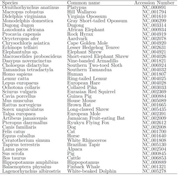
properties of this molecule. Indeed, the mitochondrial genome evolving about four times more rapidly than the nuclear genome, the recovery of the earliest divergences (37) proved to be difficult due to substitutional saturation. In particular, the first analyses of complete mitochondrial genomes created a controversy surrounding the origin of rodents that were initially found to be paraphyletic (38). Indeed, murid rodents (mice and rats) emerged first among placentals in most mitogenomic trees (39, 40). This unexpected finding was actually the result of a long-branch attraction artifact due to the fast evolving murids (41, 42, 32). Thus, for illustrative purposes, we assembled a complete mitochondrial genome data set from 38 species representing all placental orders (Table 4). The concatenation of the 12 H-stranded mitochondrial protein-coding genes (NADH Dehydrogenase subunits 1, 2, 3, 4, 4L and 5; Cytochrome c Oxydase subunits I, II and III, ATP Synthase F0 subunits 6 and 8; and Cytochrome b) led to an alignment of 3,507 amino acid sites after removing ambiguously aligned positions.
3.2 NNI heuristic search.
A ML phylogenetic model was first estimated using simultaneous NNI moves to improve a BioNJ starting tree (default option) under the mtMAM substitution model. The shape parameter (α) of a gamma distribution with four bins as well as the proportion of invariants (p-inv) were both estimated from the data. All together, the substitution model is noted mtMAM+Γ4+I. The estimated phylogeny is presented in Fig. 4.
This analysis, including the calculation of aLRT-based branch supports, took about 25 minutes to complete on an AMD Opteron 250 2.4 Ghz processor running Linux. The estimated model parameters (α = 0.69; p-inv = 0.34) indicates strong among site rate heterogeneity within the concatenation. The log likelihood of the whole phylogenetic model is -74040.38. Interestingly, three out of the four recognised major placental clades are recovered as monophyletic: Afrotheria, Xenarthra and Laurasiatheria. The fourth group, Euarchontoglires, appears paraphyletic at the base of the tree with murid rodents (Mouse and Rat) emerging first and successively followed by Guinea Pig, Squirrel, Lagomorphs (Hare and Pika) and Primates (Lemur and Human). In fact, this topology differs from what is expected to be the most accurate placental phylogeny because of the position of the murid rodent clade. This peculiar topology is reminiscent of early mitogenomic studies. It is likely to be the result of a long-branch attraction artifact that is caused by the high evolutionary rate of murid mitochondrial genomes relative to other rodents. Worth noting,
however, is the fact that the BioNJ starting topology also presents this apparent rooting artifact (not shown). This observation suggests a potential influence of the starting tree on the outcome of the NNI heuristic search. To check whether the likely artefactual topology found in Fig. 4 is a consequence of using the BioNJ topology as a starting tree for the NNI heuristic search, we conducted the same analysis using a maximum parsimony (MP) tree as the starting topology. Using this strategy results in a slightly better model with respect to the likelihood (-74040.25). The corresponding ML topology only differs from the one in Fig. 4 in the position of Bats (Fruit-eating Bat and Flying-Fox) that now emerge second within Laurasiatheria (not shown). However, as the MP topology also suffers from the rooting artifact, it is still possible that the NNI heuristic search from this starting tree may have reached a local maximum of the likelihood function.
3.3 SPR heuristic search.
The maximum likelihood phylogeny reconstructed by applying full-SPR moves to the BioNJ starting tree under the mtMAM+Γ4+I model is presented in Fig. 5. Building the tree took about 1 hour 25 minutes to complete on the same computer, which is almost exactly one hour more than the search using NNI moves. As previously, aLRT branch supports were also calculated and the time needed to work out these values was approxi-mately 5% of the total computing time. The estimated model parameters (α = 0.68; p-inv = 0.34) are almost identical to the ones obtained using the NNI search strategy. This result confirms that ML estimation of model parameters is relatively insensitive to topo-logical differences induced by the different heuristics. However, SPR moves converged to a model that has a greater log likelihood (-74021.74) than the NNI-based one (-74040.38). The SPR topology presents major differences with the NNI one since the respective mono-phyly of each of the four major placental clades is now recovered (Fig. 5). Indeed, the ML topology is no longer rooted on the Mouse/Rat ancestral branch with Euarchontoglires being monophyletic and Afrotheria now appearing as the earliest placental offshoot. This topology is almost fully compatible with the new placental phylogeny inferred from large concatenated data sets of mainly nuclear genes (34, 35, 36). This result illustrates that, in this particular case, NNI-based heuristic is trapped in a local maximum because of in-sufficient tree space exploration conditioned by the BioNJ or MP starting topologies. Note however that the NNI-based and SPR-based ML phylogenetic models are not statistically different according to a SH test (9). Hence, while simultaneous NNIs get trapped in a
local maximum, the estimated ML solution is not different from the one found by SPRs from a statistical point of view. In other words, NNI tree searching is probably trapped in this local optimum because of the lack of phylogenetic signal for certain parts of the tree.
3.4 SPR heuristic search starting from random trees.
SPR searches can also be initiated with random starting trees (see section 2.4). The full-SPR-based tree search procedure was thus repeated 10 times, each analysis starting from a different random phylogeny. In eight of these 10 replicates, the ML topology of Fig. 5 compatible with the new placental phylogeny was recovered (log-likelihood: -74021.74). However, in the two remaining replicates (20%), the SPR heuristic search converged to the alternative suboptimal topology (log-likelihood: -74040.25) that was previously found when using a MP starting tree combined with the NNI heuristic search (see section 3.2). These results suggest that the likelihood surface for this placental mitogenomic data set is dominated by at least two peaks relatively close in likelihood but distant in the space of tree topologies, one probably corresponding to the ML topology and the other to the suboptimal topology caused by the rooting artifact.
3.5 Assessing statistical support for internal edges.
Statistical supports for branches displayed by each of the two competing topologies were measured using 100 non-parametric bootstrap replicates (BP; (43)) and the approximate likelihood ratio test for branches (aLRT; (8)). BP and aLRT values (more precisely, p-values obtained from SH tests) are reported on Fig. 4 and 5 for nodes that show at least 50% bootstrap support. For both topologies, the statistical support is almost maximal for the respective monophyly of Afrotheria, Xenarthra and Laurasiatheria. The monophyly of Euarchontoglires recovered in the SPR topology (Fig. 5) is not statistically supported, as is also its paraphyly induced by the rooting artifact in the NNI topology (Fig. 4). In fact, the differences between the two topologies only involve nodes with weak support from the data.
Bootstrap and aLRT values largely agree on most branches of both trees. Indeed, branches with bootstrap supports close to 100 also have aLRT values close to 1.0 in most cases. However, a few branches are well supported according to aLRT values but have small bootstrap proportions (see the branch at the root of the Xenarthra, Afrotheria and Laurasiatheria clades, with BP=58 and aLRT=1.0). Such differences between aLRT and
bootstrap values are probably the consequence of a lack of phylogenetic signal to resolve specific parts of the phylogeny. More work still needs to be done to fully understand such result though.
4
Notes.
1. The hypothesis of site independence is relaxed in certain models. For instance, codon-based models impose a constraint on groups of columns that belong to the same codon site. Felsenstein and Churchill (44) also proposed a model where the rates of substitutions at adjacent sites are correlated. Also, several models describe the evolution of pairs of interacting nucleotides among ribosomal RNA molecules (45, 46, 47).
2. It is not very clear which of non-deterministic or deterministic approach is the best for phylogenetic inference. Note however that deterministic methods are generally faster than stochastic optimisation approaches and sufficient for numerous optimisation problems (48). On the other hand, stochastic methods have the ability to find several near-optimal trees, which gives an idea of the inferred tree variability. 3. Under the default settings, PhyML modifies the tree topology using NNI moves and
simultaneously optimises branch lengths. However, when the tree topology estimate is stable (i.e., no improvement of the likelihood can be found by modifying the current tree topology), the optimisation concentrates on branch lengths and parameters of the Markov model in order to save computing time. NNI moves with optimisation of the central and the four adjacent branch lengths are also systematically tested during the very last optimisation step. This last step frequently finds a modification of the tree topology that was not detected by the other approximate (but fast) tree topology search methods (i.e., NNI, NNI+SPR or full-SPR).
4. The SPR-search strategy implemented in PhyML 3.0 actually relies on filtering SPR moves using the parsimony criterion instead of a distance-based approach. Indeed, parsimony and likelihood are closely related from a statistical perspective and the analysis of real and simulated data (Dufayard, Guindon, Gascuel, unpublished) have demonstrated the benefits of using a parsimony-based filter.
variable if the program is launched from a command-line window. The program can also be launched by typing ‘./phyml’ provided that PhyML binary file is in the current directory. Launching PhyML by clicking on the corresponding icon is not recommended. In case PhyML can not find the sequence data file when launched by clicking on the icon, we suggest using a command-line window.
6. Questions regarding the amount of memory required can be eluded using the ‘-DBATCH’ flag when compiling the program. This option is available through a simple modifi-cation of the Makefile. It is highly recommended to use this option when launching PhyML in batch mode or when comparing run times of different programs.
7. The estimation of bases or amino-acid frequencies relies on a iterative method that takes into account gaps and ambiguous characters. The frequencies of the non-ambiguous characters (bases or amino-acids) at step n are functions of the counts of the non-ambiguous characters plus the counts of the ambiguous characters weighted by the probabilities of the non-ambiguous characters estimated at step n − 1. These probabilities correspond to the frequencies estimated at step n − 1. The same ap-proach is also used in PAML (49) and PHYLIP (12) programs.
8. PhyML uses an original method that simultaneously estimates the gamma shape pa-rameter and the proportion of invariants (Guindon and Gascuel, unpublished). This method relies on the observation that the two parameters show a strong quasi-linear positive relationship. Basically, the gamma shape parameter is first estimated using a standard one-dimensional optimisation method. The proportion of invariants is then deduced from the linear relationship with the gamma shape parameter. Hence, the estimation of the proportion of invariants does not rely on time-consuming op-timisation methods.
5
Acknowledgements
This work was supported by the ‘MITOSYS’ grant from ANR. The chapter itself is the contribution 2007-XXX of the Institut des Sciences de l’Evolution (UMR5554-CNRS)
References
[1] Felsenstein, J. (1981) Evolutionary trees from DNA sequences: a maximum likelihood approach. Journal of Molecular Evolution, 17, 368–376.
[2] Rogers, J., Swofford, D. (1999) Multiple local maxima for likelihoods of phylogenetic trees: a simulation study. Molecular Biology and Evolution, 16, 1079–1085.
[3] Huelsenbeck, J. P., Hillis, D. (1993) Success of phylogenetic methods in the four-taxon case. Systematic Biology, 42, 247–264.
[4] Swofford, D., Olsen, G., Waddel, P., Hillis, D. (1996) Phylogenetic inference. In D. Hillis, C. Moritz, B. Mable, eds., Molecular Systematics, chapter 11. Sinauer, Sunderland, MA.
[5] Guindon, S., Gascuel, O. (2003) A simple, fast and accurate algorithm to estimate large phylogenies by maximum likelihood. Systematic Biology, 52, 696–704.
[6] Olsen, G., Matsuda, H., Hagstrom, R., Overbeek, R. (1994) fastDNAml: a tool for construction of phylogenetic trees of DNA sequences using maximum likelihood. Computer Applications in the Biosciences (CABIOS), 10, 41–48.
[7] Hordijk, W., Gascuel, O. (2005) Improving the efficiency of SPR moves in phylogenetic tree search methods based on maximum likelihood. Bioinformatics, 21, 4338–4347. [8] Anisimova, M., Gascuel, O. (2006) Approximate likelihood-ratio test for branches: a
fast, accurate, and powerful alternative. Syst. Biol., 55, 539–552.
[9] Shimodaira, H., Hasegawa, M. (1999) Multiple comparisons of log-likelihoods with applications to phylogenetic inference. Molecular Biology and Evolution, 16, 1114– 1116.
[10] Jukes, T., Cantor, C. (1969) Evolution of protein molecules. In H. Munro, ed., Mam-malian Protein Metabolism, volume III, chapter 24, 21–132. Academic Press, New York.
[11] Kimura, M. (1980) A simple method for estimating evolutionary rates of base sub-stitutions through comparative studies of nucleotide sequences. Journal of Molecular Evolution, 16, 111–120.
[12] Felsenstein, J. (1993) PHYLIP (PHYLogeny Inference Package) version 3.6a2 . Dis-tributed by the author, Department of Genetics, University of Washington, Seattle. [13] Hasegawa, M., Kishino, H., Yano, T. (1985) Dating of the Human-Ape splitting by a
molecular clock of mitochondrial-DNA. Journal of Molecular Evolution, 22, 160–174. [14] Tamura, K., Nei, M. (1993) Estimation of the number of nucleotide substitutions in the control region of mitochondrial DNA in humans and chimpanzees. Molecular Biology and Evolution, 10, 512–526.
[15] Lanave, C., Preparata, G., Saccone, C., Serio, G. (1984) A new method for calculating evolutionary substitution rates. Journal of Molecular Evolution, 20, 86–93.
[16] Tavar´e, S. (1986) Some probabilistic and statistical problems on the analysis of DNA sequences. Lectures on Mathematics in the Life Sciences, 17, 57–86.
[17] Whelan, S., Goldman, N. (2001) A general empirical model of protein evolution de-rived from multiple protein families using a maximum-likelihood approach. Molecular Biology and Evolution, 18, 691–699.
[18] Dayhoff, M., Schwartz, R., Orcutt, B. (1978) A model of evolutionary change in proteins. In M. Dayhoff, ed., Atlas of Protein Sequence and Structure, volume 5, 345–352. National Biomedical Research Foundation, Washington, D. C.
[19] Jones, D., Taylor, W., Thornton, J. (1992) The rapid generation of mutation data ma-trices from protein sequences. Computer Applications in the Biosciences (CABIOS), 8, 275–282.
[20] Henikoff, S., Henikoff, J. (1992) Amino acid substitution matrices from protein blocks. Proceedings of the National Academy of Sciences of the United States of America (PNAS), 89, 10915–10919.
[21] Adachi, J., Hasegawa, M. (1996) MOLPHY version 2.3. programs for molecular phy-logenetics based on maximum likelihood. In M. Ishiguro, G. Kitagawa, Y. Ogata, H. Takagi, Y. Tamura, T. Tsuchiya, eds., Computer Science Monographs, 28. The Institute of Statistical Mathematics, Tokyo.
[22] Dimmic, M., Rest, J., Mindell, D., Goldstein, D. (2002) rtREV: an amino acid substi-tution matrix for inference of retrovirus and reverse transcriptase phylogeny. Journal of Molecular Evolution, 55, 65–73.
[23] Adachi, J., P., W., Martin, W., Hasegawa, M. (2000) Plastid genome phylogeny and a model of amino acid substitution for proteins encoded by chloroplast DNA. Journal of Molecular Evolution, 50, 348–358.
[24] Kosiol, C., Goldman, N. (2004) Different versions of the Dayhoff rate matrix. Molec-ular Biology and Evolution, 22, 193–199.
[25] Muller, T., Vingron, M. (2000) Modeling amino acid replacement. Journal of Com-putational Biology, 7, 761–776.
[26] Cao, Y., Janke, A., Waddell, P., Westerman, M., Takenaka, O., Murata, S., Okada, N., Paabo, S., Hasegawa, M. (1998) Conflict among individual mitochondrial proteins in resolving the phylogeny of eutherian orders. Journal of Molecular Evolution, 47, 307–322.
[27] Yang, Z. (1994) Maximum likelihood phylogenetic estimation from DNA sequences with variable rates over sites: approximate methods. Journal of Molecular Evolution, 39, 306–314.
[28] Gascuel, O. (1997) BIONJ: an improved version of the NJ algorithm based on a simple model of sequence data. Molecular Biology and Evolution, 14, 685–695.
[29] Posada, D., Crandall, K. (1998) Modeltest: testing the model of DNA substitution. Bioinformatics, 14, 817–918.
[30] Abascal, F., Zardoya, R., Posada, D. (2005) Prottest: selection of best-fit models of protein evolution. Bioinformatics, 21, 2104–2105.
[31] Galtier, N., Jean-Marie, A. (2004) Markov-modulated Markov chains and the covarion process of molecular evolution. Journal of Computational Biology, 11, 727–733. [32] Lin, Y.-H., McLenachan, P., Gore, A., Phillips, M., Ota, R., Hendy, M., Penny, D.
(2002) Four new mitochondrial genomes, and the stability of evolutionary trees of mammals. Molecular Biology and Evolution, 19, 2060–2070.
[33] Reyes, A., Gissi, C., Catzeflis, F., Nevo, E., Pesole, G., Saccone, C. (2004) Congru-ent mammalian trees from mitochondrial and nuclear genes using bayesian methods. Molecular Biology and Evolution, 21, 397–403.
[34] Murphy, M., Eizirik, E., O’Brien, S., Madsen, O., Scally, M., Douady, C., Teeling, E., Ryder, O., Stanhope, M., de Jong, W., Springer, M. (2001) Resolution of the early placental mammal radiation using bayesian phylogenetics. Science, 294, 2348–2351. [35] Delsuc, F., Scally, M., Madsen, O., Stanhope, M., de Jong, W., Catzeflis, F., Springer, M., Douzery, E. (2002) Molecular phylogeny of living xenarthrans and the impact of character and taxon sampling on the placental tree rooting. Molecular Biology and Evolution, 19, 1656–1671.
[36] Amrine-Madsen, H., Koepfli, K., Wayne, R., Springer, M. (2003) A new phylogenetic marker, apolipoprotein B, provides compelling evidence for eutherian relationships. Molecular Phylogenetics and Evolution, 28, 225–240.
[37] Springer, M., Bry, R. D., Douady, C., Amrine, H., Madsen, O., de Jong, W., Stan-hope., M. (2001) Mitochondrial versus nuclear gene sequences in deep-level mam-malian phylogeny reconstruction. Molecular Biology and Evolution, 18, 132–143. [38] D’Erchia, A., Gissi, C., Pesole, G., Saccone, C., Arnason, U. (1996) The guinea-pig
is not a rodent. Nature, 381, 597–600.
[39] Reyes, A., Pesole, G., Saccone, C. (1998) Complete mitochondrial DNA sequence of the fat dormouse, Glis glis: further evidence of rodent paraphyly. Molecular Biology and Evolution, 15, 499–505.
[40] Reyes, A., Pesole, G., Saccone, C. (2000) Long-branch attraction phenomenon and the impact of among-site rate variation on rodent phylogeny. Gene, 259, 177–187. [41] Philippe, H. (1997) Rodent monophyly: pitfalls of molecular phylogenies. Journal of
Molecular Evolution, 45, 712–715.
[42] Sullivan, J., Swofford, D. (1997) Are guinea pigs rodents? the importance of adequate models in molecular phylogenetics. Journal of Mammalian Evolution, 4, 77–86. [43] Felsenstein, J. (1985) Confidence limits on phylogenies: an approach using the
[44] Felsenstein, J., Churchill, G. (1996) A hidden Markov model approach to variation among sites in rate of evolution. Molecular Biology and Evolution, 13, 93–104. [45] Schniger, M., von Haesler, A. (1994) A stochastic model for the evolution of
autocor-related DNA sequences. Molecular Phylogeny and Evolution, 3, 240–247.
[46] Muse, S. (1995) Evolutionary analyses of DNA sequences subject to constraints on secondary structure. Genetics, 139, 1429–1439.
[47] Tillier, E., Collins, R. (1998) High apparent rate of simultaneous compensatory base-pair substitutions in ribosomal rna. Genetics, 148, 1993–2002.
[48] Aarts, E., Lenstra, J. K. (1997) Local search in combinatorial optimization. Wiley, Chichester.
[49] Yang, Z. (1997) PAML : a program package for phylogenetic analysis by maximum likelihood. Computer Applications in the Biosciences (CABIOS), 13, 555–556.
Figure 1. Comparison of bootstrap and SH-like branch supports, using C8 alpha chain precursor data set from TREEBASE. This data set displays a strong phylogenetic signal overall as most internal branches (13/19) have support close to their maximum values with both approaches. SH-like supports are non-significant for 5 branches (noted with ‘△’) that also have low bootstrap proportions, while one branch with a rela-tively low bootstrap proportion (72 in italic) is strongly supported according to the aLRT test (SH-like value : 0.97).
Figure 2. Text-based interface to PhyML. The PHYLIP-like text interface to the program is organised in sub-menus. The ‘+’ and ‘-’ key are used to cycle through them. For each sub-menu, the defaults options can be altered by entering the relevant keys. The data analysis is launched once the ‘y’ (or ‘Y’) key is entered.
Figure 3. Typical DNA sequence alignments (a) and input trees (b). Sequence names do not contain any blank character and at least one blank separates each name from the corresponding sequence. Trees are in standard NEWICK format.
Figure 4. ML phylogeny reconstructed using simultaneous NNI moves. The log-likelihood of the corresponding phylogenetic model is -74040.38. Numbers in the tree correspond to non-parametric bootstrap supports (100 replicates) and p-values of the ap-proximate likelihood ratios (SH-test). Values are reported only for nodes with BP > 50 and stars indicate nodes that received 100% support. S.-e. Elephant Shrew is for Short-eared Elephant Shrew.
Figure 5. ML phylogeny reconstructed using SPR moves. The log-likelihood of the corresponding phylogenetic model is -74021.74. Numbers in the tree correspond to non-parametric bootstrap supports (100 replicates) and p-values of the approximate likeli-hood ratios (SH-test). Values are reported only for nodes with BP > 50 and stars indicate nodes that received 100% support. S.-e. Elephant Shrew is for Short-eared Elephant Shrew.
Character Nucleotide Character Nucleotide A Adenosine Y C or T G Guanine K Gor T C Cytosine B C or G or T T Thymine D A or G or T U Uracil (=T ) H A or C or T M Aor C V A or C or G R Aor G − or N or X or ? unknown W A or T (=A or C or G or T ) S C or G
Table 1. List of valid characters in DNA sequences and the corresponding nucleotides.
Character Amino-Acid Character Amino-Acid
A Alanine L Leucine
R Arginine K Lysine
N or B Asparagine M Methionine
D Aspartic acid F Phenylalanine
C Cysteine P Proline
Qor Z Glutamine S Serine
E Glutamic acid T Threonine
G Glycine W Tryptophan
H Histidine Y Tyrosine
I Isoleucine V Valine
L Leucine − or X or ? unknown
K Lysine (can be any amino acid)
Table 2. List of valid characters in protein sequences and the corresponding amino acids.
Sequence file name : ‘seq’
Output file name Content
seq phyml tree.txt ML tree
seq phyml stats.txt ML model parameters
seq phyml boot trees.txt ML trees – bootstrap replicates
seq phyml boot stats.txt ML model parameters – bootstrap replicates
seq phyml best tree.txt best ML tree – multiple random starts
Species Common name Accession Number
Ornithorhynchus anatinus Platypus NC 000891
Macropus robustus Hill Wallaroo NC 001794
Didelphis virginiana Virginia Opossum NC 001610
Monodelphis domestica Gray Short-tailed Opossum NC 006299
Dugong dugon Dugong NC 003314
Loxodonta africana African Elephant NC 000934
Procavia capensis Rock Hyrax NC 004919
Orycteropus afer Aardvark NC 002078
Chrysochloris asiatica Cape Golden Mole NC 004920
Echinops telfairi Lesser Hedgehog Tenrec NC 002631
Elephantulus sp. Elephant Shrew NC 004921
Macroscelides proboscideus Short-eared Elephant Shrew NC 004026
Dasypus novemcinctus Nine-banded Armadillo NC 001821
Choloepus didactylus Southern Two-toed Sloth NC 006924
Tamandua tetradactyla Southern Tamandua NC 004032
Homo sapiens Human NC 001807
Lemur catta Ring-tailed Lemur NC 004025
Lepus europaeus European Hare NC 004028
Ochotona collaris Collared Pika NC 003033
Sciurus vulgaris Eurasian Red Squirrel NC 002369
Cavia porcellus Guinea Pig NC 000884
Mus musculus House Mouse NC 005089
Rattus norvegicus Brown Rat NC 001665
Sorex unguiculatus Long-clawed Shrew NC 005435
Talpa europaea European Mole NC 002391
Artibeus jamaicensis Jamaican Fruit-eating Bat NC 002009
Pteropus dasymallus Ryukyu Flying Fox NC 002612
Canis familiaris Dog NC 002008
Felis catus Cat NC 001700
Equus caballus Horse NC 001640
Ceratotherium simum White Rhinoceros NC 001808
Tapirus terrestris Brazilian Tapir NC 005130
Lama pacos Alpaca NC 002504
Sus scrofa Pig NC 000845
Bos taurus Cattle NC 006853
Hippopotamus amphibius Hippopotamus NC 000889
Balaenoptera physalus Finback Whale NC 001321
Lagenorhynchus albirostris White-beaked Dolphin NC 005278
Table 4. List of the mammalian species and the corresponding GenBank acces-sion numbers of the complete mitochondrial genomes that were analysed in this chapter (see Section 3.1).
SEQ1 SEQ2 SEQ3 SEQ4 SEQ5 SEQ6 SEQ7 SEQ8 SEQ9 SEQ10 SEQ11 SEQ12 SEQ13 SEQ14 SEQ15 SEQ16 SEQ17 SEQ18 SEQ19 SEQ20 SEQ21 SEQ22 SEQ23 SEQ24 100/1.00 100/1.00 100/1.00 100/1.00 100/1.00 100/1.00 100/1.00 100/1.00 99/0.98 75/0.62 99/0.99 100/0.98 100/0.99 97/0.98 36/0.16 61/0.65 61/0.30 95/0.94 91/0.95 72/0.97
△
△
△
△
△
Figure 1.a) 5 60 first_seq_name CCATCTCACGGTCGGTACGATACACCKGCTTTTGGCAGGAAATGGTCAATATTACAAGGT second_seq_name CCATCTCACGGTCAG---GATACACCKGCTTTTGGCGGGAAATGGTCAACATTAAAAGAT third_seq_name RCATCTCCCGCTCAG---GATACCCCKGCTGTTG????????????????ATTAAAAGGT fourth_seq_name RCATCTCATGGTCAA---GATACTCCTGCTTTTGGCGGGAAATGGTCAATCTTAAAAGGT fifth_seq_name RCATCTCACGGTCGGTAAGATACACCTGCTTTTGGCGGGAAATGGTCAAT????????GT 5 40 first_seq_name CCATCTCANNNNNNNNACGATACACCKGCTTTTGGCAGG second_seq_name CCATCTCANNNNNNNNGGGATACACCKGCTTTTGGCGGG third_seq_name RCATCTCCCGCTCAGTGAGATACCCCKGCTGTTGXXXXX fourth_seq_name RCATCTCATGGTCAATG-AATACTCCTGCTTTTGXXXXX fifth_seq_name RCATCTCACGGTCGGTAAGATACACCTGCTTTTGxxxxx b) ((first_seq_name:0.03,second_seq_name:0.01):0.04,third_seq_name:0.01,(fourth_seq_name:0.2,fifth_seq_name:0.05)); ((third_seq_name:0.04,second_seq_name:0.07):0.02,first_seq_name:0.02,(fourth_seq_name:0.1,fifth_seq_name:0.06)); Figure 3.
0.1 substitution / site Platypus Wallaroo Short-tailed Opossum Virginia Opossum 99/1.0 Rat Mouse Guinea Pig Squirrel Pika Hare Lemur Human 91/0.98 Armadillo Anteater Sloth 77/0.74 Hyrax Dugong Elephant 70/0.69 99/1.0 Tenrec Aardvark Golden Mole Elephant Shrew
S.-e. Elephant Shrew
64/0.80 51/0.26 69/0.68 93/1.0 Shrew Mole Cat Dog Horse Rhino Tapir 60/0.52 60/0.76 Fruit-eating Bat Flying Fox Pig Alpaca Cattle Hippo Dolphin Whale 84/0.91 94/0.97 73/0.82 69/0.97 58/1.0 * XENARTHRA LAURASIA THERIA * * * * * * * * * * * * AFRO THERIA EUARCHONTO GLIRES MARSUPIALIA MONOTREMATA Figure 4.
XENARTHRA LAURASIA THERIA AFRO THERIA EUARCHONTO GLIRES MARSUPIALIA MONOTREMATA 0.1 substitution / site 99/1.0 65/0.62 61/0.86 56/0.32 68/0.56 99/0.98 77/0.79 87/0.98 67/0.45 54/0.72 89/0.89 93/0.98 78/0.85 59/0.08 61/0.35 * * Platypus Wallaroo Short-tailed Opossum Virginia Opossum * * Hyrax Dugong Elephant Tenrec Aardvark Golden Mole Elephant Shrew
S.-e. Elephant Shrew Armadillo Anteater Sloth * * * Lemur Human Rat Mouse Guinea Pig Squirrel Pika Hare * * * * * * * Shrew Mole Cat Dog Horse Rhino Tapir Fruit-eating Bat Flying Fox Pig Alpaca Cattle Hippo Dolphin Whale Figure 5.