Cyclic asymptotic behaviour of a population reproducing by fission into two equal parts

HAL Id: hal-01363549

https://hal.archives-ouvertes.fr/hal-01363549v5

Submitted on 17 Nov 2018

HAL is a multi-disciplinary open access

archive for the deposit and dissemination of

sci-entific research documents, whether they are

pub-lished or not. The documents may come from

L’archive ouverte pluridisciplinaire HAL, est

destinée au dépôt et à la diffusion de documents

scientifiques de niveau recherche, publiés ou non,

émanant des établissements d’enseignement et de

Cyclic asymptotic behaviour of a population

reproducing by fission into two equal parts

Etienne Bernard, Marie Doumic, Pierre Gabriel

To cite this version:

Etienne Bernard, Marie Doumic, Pierre Gabriel. Cyclic asymptotic behaviour of a population

repro-ducing by fission into two equal parts. Kinetic and Related Models , AIMS, 2019, 12 (3), pp.551-571.

�10.3934/krm.2019022�. �hal-01363549v5�

Cyclic asymptotic behaviour of a population

reproducing by fission into two equal parts

´

Etienne Bernard

Marie Doumic

Pierre Gabriel

November 19, 2018

Abstract

We study the asymptotic behaviour of the following linear growth-fragmentation equation

B

Btupt, xq ` B

Bx`xupt, xq˘ ` Bpxqupt, xq “ 4Bp2xqupt, 2xq, and prove that under fairly general assumptions on the division rate Bpxq, its solution converges towards an oscillatory function, explicitely given by the projection of the initial state on the space generated by the count-able set of the dominant eigenvectors of the operator. Despite the lack of hypocoercivity of the operator, the proof relies on a general relative en-tropy argument in a convenient weighted L2 _{space, where well-posedness}

is obtained via semigroup analysis. We also propose a non-diffusive nu-merical scheme, able to capture the oscillations.

Keywords: growth-fragmentation equation, self-similar fragmentation, long-time behaviour, general relative entropy, periodic semigroups, non-hypocoercivity MSC 2010: (Primary) 35Q92, 35B10, 35B40, 47D06, 35P05 ; (Secondary) 35B41, 92D25, 92B25

Introduction

Over the last decades, the mathematical study of the growth-fragmentation equation and its linear or nonlinear variants has led to a wide literature.

Several facts explain this lasting interest. First, variants of this equation are used to model a wide range of applications, from the internet protocol suite ∗_{Laboratoire de G´eod´esie, IGN-LAREG, Bˆatiment Lamarck A et B, 35 rue H´el`ene Brion,}

75013 Paris. Email: etienne.bernard@ign.fr

†_{Sorbonne Universit´es, Inria, UPMC Univ Paris 06, Mamba project-team, Laboratoire}

Jacques-Louis Lions. Email adress: marie.doumic@inria.fr

‡_{Wolfgang Pauli Institute, c/o Faculty of Mathematics of the University of Vienna} §_{Laboratoire de Math´ematiques de Versailles, UVSQ, CNRS, Universit´e Paris-Saclay, 45}

to cell division or polymer growth; it is also obtained as a useful rescaling for the pure fragmentation equation (then the growth rate is linear). Second, despite the relative simplicity of such a one-dimensional equation, the study of its behaviour reveals complex and interesting interplays between growth and division, and a kind of dissipation even in the absence of diffusion. Finally, the underlying stochastic process has also - and for the same reasons - raised much interest, and only recently have the links between the probabilistic approach and the deterministic one begun to be investigated.

In its general linear form, the equation may be written as follows

B Btupt, xq ` B Bx`gpxqu˘ ` Bpxqupt, xq “ 8 ż x

kpy, xqBpyqupt, yqdy, (GF)

where upt, xq represents the concentration of individuals of size x ě 0 at time t, gpxq ě 0 their growth rate, Bpxq ě 0 their division rate, and kpy, xq ě 0 the quantity of individuals of size x created out of the division of individuals of size y.

The long-time asymptotics of this equation has been studied and improved in many successive papers. Up to our knowledge, following the biophysical pioneering papers [9, 8, 35], the first mathematical study was carried out in [15], where the equation was considered for the mitosis kernel / binary fis-sion (kpy, xq “ 2δx“y₂) in a compact set x P rα, βs. The authors proved the

central behaviour of the equation, already conjectured in [9]: under balance and regularity assumptions on the coefficients, there exists a unique dominant eigenpair pU pxq ě 0, λ ą 0q such that upt, xqe´λt _{Ñ U pxq in a certain sense,}

with an exponential speed of convergence. In [15], the proofs were based on semigroup methods and stated for the space of continuous functions provided with the supremum norm. Many studies followed: some of them, most notably and recently [31], relaxing the previous assumptions in the context of semigroup theory [2, 5, 6, 7, 19, 22]; others deriving explicit solutions [25, 37, 38] or intro-ducing new methods - one of the most elegant and powerful being the General Relative Entropy [30], leading to convergence results in norms weigthed by the adjoint eigenproblem. However, though in some cases the entropy method may lead to an explicit spectral gap in some integral norm [34, 28, 32], or when the coefficients are such that an entropy-entropy dissipation inequality exists [13, 3], in general it fails to provide a rate of convergence.

On the margins of this central behaviour, some papers investigated non-uniqueness [4] or other kinds of asymptotics, happening for instance when the balance or mixing assumptions between growth and division fail to be satisfied: e.g. when the fragmentation dominates the growth [6, 11, 12, 24, 16]. A stronger “memory” of the initial behaviour may then be observed, contrary to the main case, where the only memory of the initial state which remains asymptotically is a weighted average.

Among these results, the case when the growth rate is linear, i.e. gpxq “ x, and the mother cell divides into two equal offspring, i.e. kpy, xq “ 2δx“x

a special place, both for modelling reasons - it is the emblematic case of idealised bacterial division cycle, and also the rescaling adapted to the pure fragmentation equation - and as a limit case where the standard results fail to be true. The equation is then $ ’ & ’ % B Btupt, xq ` B

Bx`xupt, xq˘ ` Bpxqupt, xq “ 4Bp2xqupt, 2xq, x ą 0, up0, xq “ uin

pxq.

(1)

In 1967, G. I. Bell and E. C. Anderson already noted [9]:

”If the rate of cell growth is proportional to cell volume, then (...) a daughter cell, having just half the volume of the parent cell, will grow at just half the rate of the parent cell. It follows that if one starts with a group of cells of volume V , age r, at time 0, then any daughter cell of this group, no matter when formed, will always have a volume equal to half the volume of an undivided cell in the group. There will then be no dispersion of cell volumes with time, and the population will consist at any time of a number of cell generations differing by just a factor of 2 in volume. For more general initial conditions, the population at late times will still reflect the initial state rather than simply growing exponentially in time. ”

After [9], the reason for this specific behaviour was stated in [15, 26]: instead of a unique dominant eigenvalue, there exists a countable set of dominant eigen-values, namely 1 ` 2iπ

log 2Z. O. Diekmann, H. Heijmans and H. Thieme explain

in [15]:

The total population size still behaves like ret

s but convergence in shape does not take place. Instead the initial size distribution turns around and around while numbers are multiplied. (...) The following Gedanken experiment illustrates the bio-logical reason. Consider two cells A and B with equal size and assume that at some time instant t0 cell A splits into a and a. During the time interval rt0, t1s, a, a and B

grow and at t1 cell B splits into b and b. If gpxq “ cx, the daughter cells a and b will

have equal sizes just as their mothers A and B. ln other words, the relation ”equal size” is hereditary and extends over the generations. The growth model behaves like a multiplicating machine which copies the size distribution.

In [22], G. Greiner and R. Nagel are the first to prove this long-time periodic behaviour. They use the theory of positive semigroups combined with spectral analysis to get the convergence to a semigroup of rotations. The method relies on some compactness arguments, which force the authors to set the equation on a compact subset of p0, 8q (x P rα, βs with α ą 0).

In the present paper, we extend the result to the equation set on the whole R`. Additionally, we determine explicitly the oscillatory limit by the

means of a projection of the initial condition on the dominant eigenfunctions. Our method relies on General Relative Entropy inequalities (Section 1), which unexpectedly may be adapted to this case and which are the key ingredient for an explicit convergence result (Theorem 2 in Section 2, which is the main result of our study). We illustrate our results numerically in Section 3, proposing a non-diffusive scheme able to capture the oscillations.

1

Eigenvalue problem and Entropy

To study the long time asymptotics of Equation (1), we elaborate on previously established results concerning the dominant positive eigenvector and general relative entropy inequalities.

1.1

Dominant eigenvalues and balance laws

The eigenproblem and adjoint eigenproblem related to Equation (1) are λU pxq ``xUpxq˘1` BpxqU pxq “ 4Bp2xqU p2xq, (2) λφpxq ´ xφ1 pxq ` Bpxqφpxq “ 2Bpxqφ ´_x 2 ¯ . (3)

Perron eigenproblem consists in finding positive solutions U to (2), which in general give the asymptotic behaviour of time-dependent solutions, which align along eλtU pxq. Recognizing here a specific case of the eigenproblem studied in [17], we work under the following assumptions:

$ ’ ’ ’ ’ & ’ ’ ’ ’ % B : p0, 8q Ñ p0, 8q is locally integrable, Dz0, γ0, K0ą 0, @x ă z0, Bpxq ď K0xγ0, Dz1, γ1, γ2, K1, K2ą 0, @x ą z1, K1xγ1ď Bpxq ď K2xγ2. (4)

We then have the following result, which is a particular case of [17, Theorem 1]. Theorem 1. Under Assumption (4), there exists a unique positive eigenvector U P L1

pR`q to (2) normalised by

ş8

0 x U pxqdx “ 1. It is related to the eigenvalue

λ “ 1 and to the adjoint eigenvector φpxq “ x solution to (3). Moreover, xα_{U P L}8

pR`q for all α P R, and U P W1,1pR`q.

As already noticed in [15], though 1 is the unique eigenvalue related to a positive eigenvector, here it is not the unique dominant eigenvalue: we have a set of eigentriplets pλk, Uk, φkq with k P Z defined by

λk“ 1 ` 2ikπ log 2, Ukpxq “ x ´2ikπ<sub>log 2U pxq, φ</sub> kpxq “ x1` 2ikπ log 2_{. (5)}

This is the first difference with the most studied case, where the Perron eigen-value happens to be the unique dominant one: here all these eigeneigen-values have a real part equal to 1, so that they all belong to the peripheral spectrum. The natural questions which emerge are to know whether this set of dominant eigen-vectors is attractive, as it is the case when it is formed by a unique function; and if so, where the proofs are different.

First we notice an important property: the family `pUkqkPZ, pφkqkPZ

˘ is biorthogonal for the bracket

xf, ϕy :“ ż8

0

which means that

@pk, lq P Z2, xUk, φly “ δkl. (6)

This is a direct consequence of the normalization of the Perron eigenvectors which writes xU , φy “ 1 and the fact that λk ‰ λl for k ‰ l.

Even though we are interested in real-valued solutions to Equation (1), due to the fact that the dominant eigenelements have nonzero imaginary part, we have to work in spaces of complex-valued functions. Of course real-valued so-lutions are readily obtained from complex-valued soso-lutions by taking the real or imaginary part. From now on when defining functional spaces we always consider measurable functions from R` to C.

The biorthogonal property (6) can be extended into balance laws for general solutions to Equation (1). For uin P L1pφpxqdxq and u P CpR`, L1pφpxqdxqq

solution to (1) we have the conservation laws

@k P Z, @t ě 0, xupt, ¨q, φky e´λkt“ xuin, φky. (7)

1.2

General Relative Entropy inequalities

Additionally to the conservation laws above, we have a set of entropy inequal-ities. In this section, we remain at a formal level. Rigorous justification of the stated results will appear once the existence and uniqueness results are estab-lished.

Lemma 1 (General Relative Entropy Inequality). Let B satisfy Assump-tion (4), U be the Perron eigenvector defined in Theorem 1 and upt, xq be a solution of Equation (1). Let H : C Ñ R` be a positive, differentiable and

convex function. Provided the quantities exist, we have d dt 8 ż 0 x U pxqH´upt, xq U pxqet ¯ dx “ ´DHruptqe´ts ď 0, with DH _{defined by} DHrus :“ 8 ż 0 xBpxq U pxq „ H´up x 2q U px 2q ¯ ´ H ´upxq U pxq ¯ ´ ∇H ´_upxq U pxq ¯ ¨ ´upx 2q U px 2q ´upxq U pxq ¯ dx, where ∇H is the gradient of H obtained by identifying C with R2_{and ¨ stands for}

the canonical inner product in R2

. Moreover, for H strictly convex, u : R`Ñ C

satisfies DH

rus “ 0 iff it is such that upxq

U pxq “ up2xq

U p2xq, a.e. x ą 0. In particular, for all k P Z, DHrUks “ 0.

The proof is immediate and now standard, carried out by calculation term by term and use of the equations (1), (2) and (3), see for instance [33, p.92].

In the cases where the Perron eigenvector is a unique dominant eigenvector, the entropy inequality is a key step to obtain the convergence of upt, xqe´t

towards xuin, φy U pxq. The idea is to prove that upt, xqe´t_{tends to a limit u} 8

such that DH

ru8s “ 0, which in general implies that u8 is proportional to U ;

the conservation law then giving the proportionality constant.

Here however, since any function vpxq “ f plog xqU pxq with f log 2-periodic satisfies DH

rvs “ 0, the usual convergence result does not hold. This is due to the lack of hypocoercivity in our case. It is known from [13, 3, 21] that the general form (GF) of the growth-fragmentation equation is coercive for par-ticular choices of the coefficients, in the sense that the differential inequality

d

dt}upt, ¨q} ď ´ν}upt, ¨q} holds for some positive constant ν and a well-chosen

norm } ¨ }, when uin _{is such that xu}in_{, φy “ 0. As already noticed in [28] such}

an inequality cannot be valid for an entropic norm in the case of equal mito-sis. Indeed if for some time t ě 0 (for instance t “ 0) the solution satisfies upt, xq{U pxq “ upt, 2xq{U p2xq, then the time derivative of the norm vanishes. However in this case the equation can be hypocoercive in the sense (see [36]) that }upt, ¨q} ď Ce´νt_}uin

} holds for some positive constants C, ν and any initial distribution satisfying xuin_{, φy “ 0. This result is proved in [31, 10] for a class}

of weighted L1 _{norms in the case of a constant growth rate g. Roughly}

speak-ing this situation of a non-coercive but hypocoercive equation appears when the dissipation of entropy can vanish for a nontrivial set of functions, but this set is unstable for the dynamics of the equation. In our case the equation is not hypocoercive because the set of functions with null entropy dissipation is invariant under the flow, as expressed by the following lemma.

Lemma 2. Consider a strictly convex function H and let upt, xq be the solution to Equation (1) with initial condition up0, xq “ uin

pxq. We have the invariance result

DHruins “ 0 ùñ DHrupt, ¨qs “ 0, @t ě 0.

As Lemma 1, Lemma 2 is valid in a space where the existence and unique-ness of a solution is proved, as for instance in the space L2pR`, x{U pxqdxq, see

Section 2.

Proof. Let uin _{such that D}H

ruins “ 0 and denote upt, ¨q the solution to Equa-tion (1).

We have already seen in Lemma 1 that for any u : R`Ñ C, we have

DHrus “ 0 ðñ upxq U pxq “ up2xq U p2xq, a.e. x ą 0, so that by assumption u_{U pxq}inpxq “ u in_p2xq

U p2xq for almost every x ą 0.

To prove Lemma 2 we thus want to prove that upt,xq_{U pxq} “ upt,2xq_{U p2xq} for almost every x ą 0, t ą 0. To do so, we notice that if we have a solution ˜u of Equation (1)

which satisfies this property, then the ration vpt, xq “ ˜upt, xq{U pxqe´t_{is solution}

of the following simple transport equation

Btvpt, xq ` xBxvpt, xq “ 0,

so that vpt, xq “ vp0, xe´t_{q. We are led to define a function u} 1by

u1pt, xq :“ uinpxe´tq

U pxq et

U pxe´t_q.

We easily check that u1pt, xq{U pxq “ u1pt, 2xq{U p2xq for all t and almost all x,

and that u1 is solution to Equation (1). We conclude by uniqueness that we

have u ” u1 and so DHrupt, ¨qs “ 0 for all t ě 0.

For Hpzq “ |z|p_{the entropy corresponds to the p-power of the norm in}

Ep:“ LppR`, φpxqU1´ppxq dxq.

Define also the space

E8:“ u : R`Ñ C measurable, DC ą 0, |u| ď CU a.e.(,

which is the analogous of Ep for p “ 8, endowed with the norm

}u}E8:“ sup ess

xą0

|upxq| U pxq.

These spaces have the property to be invariant under the dynamics of Equa-tion (1) and to constitute a tower of continuous inclusions, as it is made more precise in the following two lemmas.

Lemma 3. Let p P r1, 8s and let upt, xq be the solution to Equation (1) with initial data uin

P Ep. Then upt, ¨q P Ep for all t ě 0 and

}upt, ¨qe´t}Epď }u

in

}Ep.

Proof. For p ă 8, this is a direct consequence of Lemma 1 by considering the convex function Hpzq “ |z|p. Similarly for p “ 8 we get the result by applying Lemma 1 with the convex function

Hpzq “ # |z| ´ C if |z| ě C 0 if |z| ď C with C “ }uin }E8.

Lemma 4. Let 1 ď p ď q ď 8 and u P Eq. Then u P Ep and

Proof. It is clear if q “ `8. For q ă `8, since φpxq U pxqdx is a probability measure the Jensen’s inequality ensures that

}u}qEp“ ˆ ż _ˇ ˇ ˇ u U ˇ ˇ ˇ p φ U ˙q{p ď ż ˇ ˇ ˇ u U ˇ ˇ ˇ q φ U “ }u}qEq.

2

Convergence in the quadratic norm

Equipped with the General Relative Entropy inequalities, we now combine them with Hilbert space techniques to prove the convergence to periodic solutions. The Hilbert space formalism provides an interpretation of the periodic limit in terms of Fourier decomposition, and allows us to give the main ingredients of the proof while avoiding too many technicalities. We first introduce the Hilbert space (Section 2.1), in which we prove the well-posedness of Equation (1) (Section 2.2). We state our main result in Theorem 2.

2.1

The Hilbert space

As we will see below, working in a Hilbert setting is very convenient for our study. Drawing inspiration from the General Relative Entropy with the convex quadratic function Hpzq “ |z|2, we work in the Hilbert space

E2“ L2pR`, x{U pxq dxq

endowed with the inner product

pf, gq :“ ż8

0

f pxqgpxq x U pxqdx. We denote by } ¨ } the corresponding norm defined by

}f }2“ pf, f q.

In this space, the normalization we have chosen for U means }U } “ }Uk} “ 1

and the biorthogonality property (6) reads

pUk, Ulq “ xUk, φly “ δk,l,

meaning that pUkqkPZ is an orthonormal family in E2. As a consequence the

family pUkqkPZis a Hilbert basis of the Hilbert space

and the orthogonal projection on this closed subspace of E2is given by P u :“ `8 ÿ k“´8 pu, UkqUk, @u P E2.

Additionally, we have the Bessel’s inequality

}P u}2“

`8

ÿ

k“´8

|pu, Ukq|2ď }u}2.

As it is stated in the following lemma, there is a crucial link between X and the quadratic dissipation of entropy (i.e. DH

rus for Hpzq “ |z|2), which can be written in a simpler way as

D2rus “ ż8 0 xBpxq U pxq ˇ ˇ ˇ ˇ upxq U pxq ´ upx{2q U px{2q ˇ ˇ ˇ ˇ 2 dx. (8) Lemma 5. We have X “ tu P E2, D2rus “ 0u.

Proof. Since |z|2 _{is strictly convex, we have already seen in Lemma 1 (and it is}

even clearer in the case of D2_{) that}

tu P E2, D2rus “ 0u “ tu P E2, upxq{U pxq “ up2xq{U p2xq, a.e. x ą 0u Ą X.

Also we clearly have

tu P E2, upxq{U pxq “ up2xq{U p2xq, a.e. x ą 0u “

tu P E2, Df : R Ñ C log 2-periodic, upxq “ f plog xqUpxq, a.e. x ą 0u.

If u P E2 is of the form upxq “ f plog xqU pxq with f : R Ñ C log 2-periodic

then necessarily f P L2

pr0, log 2sq and the Fourier theory ensures (Fourier-Riesz-Fischer theorem) that

f pyq “

`8

ÿ

k“´8

ˆ

f pkqe2ikπylog 2 _,

where ˆ f pkq “ 1 log 2 żlog 2 0

f pyqe´2ikπylog 2 _{dy P `}2_pZq.

So we have in L2 locp0, 8q upxq “ U pxq `8 ÿ k“´8 ˆ f pkqx2ikπlog 2 <sub>“</sub> `8 ÿ k“´8 ˆ f p´kqUkpxq P X.

2.2

Well-posedness of the Cauchy problem

Since the Perron eigenvalue λ “ 1 is strictly positive, it is convenient to consider a rescaled version of our problem

$ ’ & ’ % B Btvpt, xq ` B Bx`xvpt, xq˘ ` vpt, xq ` Bpxqvpt, xq “ 4Bp2xqvpt, 2xq, x ą 0, vp0, xq “ uin pxq. (9) The solutions to Equation (1) are related to the solutions to (9) by the simple relation

upt, xq “ etvpt, xq.

It is proved in [20] (see also [10]) that the problem (9) is well-posed in E1 and

admits an associated C0-semigroup pTtqtě0 which is positive, meaning that for

any uin

P E1there exists a unique (mild) solution v P CpR`, E1q to (9) which is

given by vptq “ Ttuin, and vptq ě 0, t ě 0, for uině 0. From Lemma 3 we have

that all subspaces Ep with p P r1, 8s are invariant under pTtqtě0. Additionally,

the restriction of Ttto any Ep is a contraction, i.e.

@u P Ep, @t ě 0, }Ttu}Epď }u}Ep. (10)

To get the well-posedness of (9) in E2, it only remains to check the strong

continuity of pTtqtě0in E2.

Lemma 6. The semigroup pTtqtě0 restricted to E2 is strongly continuous.

Proof. We use the subspace E₈ Ă E2and the contraction property (10) to write

for any u P E8 }Ttu ´ u}2E2 “ ż8 0 |Ttu ´ u|2pxq x U pxqdx ď 2}u}E8 ż8 0 |Ttu ´ u|pxqx dx “ 2}u}E8}Ttu ´ u}E1.

The strong continuity of pTtqtě0 in E1 ensures that }Ttu ´ u}E1 Ñ 0 and so

}Ttu ´ u}E2 Ñ 0 when t Ñ 0. By density of E8 Ă E2 we get the strong

continuity of pTtqtě0in E2.

We denote by A the generator of the semigroup pTtqtě0in E2. For any u in

the domain DpAq we have in the distributional sense Aupxq “ ´pxupxqq1

´ upxq ´ Bpxqupxq ` 4Bp2xqup2xq.

The eigenpairs pλk, Ukq are defined by A Uk “ pλk´ 1q Uk and we easily prove

the following properties.

1. @k P Z, TtUk“ e 2ikπt log 2 U_k, 2. @u P E2, @k P Z, pTtu, Ukq “ pu, Ukqe 2ikπt log 2 _, 3. @u P E2, P Ttu “ TtP u “ř_kPZpu, Ukqe 2ikπt log 2U_k,

4. TtX Ă X and for all u P X, Ttu “ř_kPZpu, Ukqe

2ikπt log 2 U_k,

5. X Ă DpAq and for all u P X, Au “ř

kPZpu, Ukq2ikπ_{log 2}Uk.

The second property is nothing but a rewriting of the conservation laws (7). The fourth point makes more precise and proves more rigorously the invariance property in Lemma 2.

2.3

Convergence

We are now ready to state the asymptotic behaviour of solutions to Problem 1. Theorem 2. Assume that B satisfies Hypothesis (4) and define Uk by (5).

Then for any uinP E2, the unique solution upt, xq P C

` R`, E2˘ to Equation (1) satisfies 8 ż 0 ˇ ˇ ˇ ˇupt, xqe ´t ´ `8 ÿ k“´8 puin, Ukqe 2ikπ log 2tU<sub>kpxq</sub> ˇ ˇ ˇ ˇ 2 x dx U pxq ÝÝÝÝÑtÑ`8 0.

Remark 1. This convergence result can also be formulated in terms of semi-groups. Set Rtu :“ TtP u “ P Ttu “ 8 ÿ k“´8 pu, Ukqe 2ikπ log 2tU_k.

This defines a semigroup,

Rt`su “ Tt`sP u “ Tt`sP2u “ TtTsP2u “ TtP TsP u “ RtRsu,

which is log 2-periodic. The result of Theorem 2 is equivalent to the strong convergence of pTtqtě0to pRtqtě0, i.e.

@u P E2, }Ttu ´ Rtu} ÝÝÝÝÑ tÑ`8 0.

It is also equivalent to the strong stability of pTtqtě0 in XK“ Ker P

@u P XK, }Ttu} ÝÝÝÝÑ tÑ`8 0.

Remark 2. We may use the Poisson summation formula to reinterpret the limit function in terms of only uinpxq : we recall that this formula states that, under proper assumptions on f and its Fourier transform F f pξq “

`8

ş

´8

f pyqe´iyξ_dy,

we have 8 ÿ `“´8 f py ` `aq “ 8 ÿ k“´8 F f p2πk a qe 2ikπy a .

Taking a “ log 2, f pyq “ uinpe´yqe´2y, we apply it to the limit function taken in y “ t ´ log x 8 ÿ k“´8 puin, UkqUkpxqe 2ikπt log 2 _{“ U pxq} 8 ÿ `“´8 2´2`x2e´2tuinp2´`xe´tq.

This formula is reminiscent of a similar one found in [16], Theorem 1.3. (b), for the limit case B constant.

Proof of Theorem 2. We follow here the classical proof of convergence, pio-neered in [29, 30]. Though the limit is now an oscillating function, this strategy may be adapted here, as shown below.

Define hpt, xq :“ upt, xqe´t ´ `8 ÿ k“´8 puin, Ukqe 2ikπ log 2tU_{kpxq “ pI ´ P qTt}uin

which is solution to Equation (2.2). Lemma 3 with p “ 2 ensures that d

dt}hpt, ¨q} ď 0,

so that it decreases through time. Since it is a nonnegative quantity, it means that it tends toward a limit L ě 0 and it remains to show that L “ 0. Let us adapt to our case the proof in B. Perthame’s book [33, p.98]. Because of the contraction property, it is sufficient to do so for uin

P DpAq which is a dense subspace of E2. Recall that for uinP DpAq the solution to Equation (1) can be

understood as a classical solution, upt, ¨q belonging to DpAq for all time. The last property in Proposition 7 ensures that X Ă DpAq, so hp0, ¨q P DpAq. Define qpt, xq “ Bthpt, xq which is clearly a mild solution to Equation (1) with initial

datum

qpt “ 0, xq “ Ahpt “ 0, xq. By contraction we get

}qpt, ¨q} ď }Ahp0, ¨q}.

Introduce the sequence of functions hnpt, ¨q “ hpt ` n, ¨q. Since h and Bth are

uniformly bounded in the Hilbert space E2, the Ascoli and Banach-Alaoglu

the-orems ensure that phnqnPNis relatively compact in Cpr0, T s, E2wq where E2wis E2

hn, we have hn Ñ g in Cpr0, T s, E2wq. Additionally since ş8 0 D 2 rhpt, ¨qs dt ă `8, we have żT 0 D2rhnpt, ¨qs dt “ żT `n n D2rhpt, ¨qs dt Ñ 0. and it ensures, using the definition (8) of D2_{, that} hnpt,xq

U pxq ´ hnpt,2xq

U p2xq Ñ 0 in

the distributional sense. We deduce from the convergence hnÑ g that gpt,xq_{U pxq} ´ gpt,2xq

U p2xq “ 0, and so D 2

rgpt, ¨qs “ 0 for all t ě 0. By Lemma 5 this means that gpt, ¨q P X for all t ě 0. But for all n P N and all t ě 0 we have hnpt, ¨q P XK“

KerP by construction of h, and since XK_{is a linear subspace, the weak limit g}

of hn also satisfies gpt, ¨q P XK for all t ě 0. Finally gpt, ¨q P X X XK“ t0u for

all t ě 0, so g ” 0 and the proof is complete.

The result in Theorem 2 is in contrast to the property of asynchronous exponential growth which states that the solutions behave like upt, xq „ xuin, φy U pxqet when t Ñ `8. This property is satisfied for a large class of growth-fragmentation equations [30], but the lack of hypocoercivity in our case prevents it to hold. However we can deduce from Theorem 2 a “mean asynchronous exponential growth” property, in line with probabilistic results, e.g. [18].

Corollary 1. Under Assumption (4), the semigroup pTtqtě0 generated by

pA, DpAqq is mean ergodic, i.e.

@u P E2, 1 t żt 0 Tsu ds ÝÝÝÝÑ

tÑ`8 P0u “ pu, U q U “ xu, φy U .

Proof. Because of Theorem 2, it suffices to prove that 1 t żt 0 Rsu ds “ P ˆ 1 t żt 0 Tsu ds ˙ ÝÝÝÝÑ tÑ`8 P0u. Denoting mt“1_t şt

0Tsu ds the Ces`aro means of pTtuqtě0 we have

P mt“ `8

ÿ

k“´8

pmt, UkqUk.

By the conservation laws (7) we have for k ‰ 0

pmt, Ukq “ 1 t żt 0 pTsu, Ukq ds “ pu, Ukq 1 t żt 0

e2ikπlog 2s_{ds “ pu, Ukq}log 2

2ikπ

e2ikπlog 2t_{´ 1}

t and pmt, U0q “ pu, U0q. This gives

P mt“ P0u ` 1 t ÿ k‰0 pu, Ukq log 2 2ikπ Uk`e 2ikπ log 2t´ 1˘.

Since › › › › ÿ k‰0 pu, Ukq log 2 2ikπ Uk`e 2ikπ log 2t<sub>´ 1</sub>˘ › › › › 2 “ ÿ k‰0 ˇ ˇ ˇpu, Ukq log 2 2ikπ`e 2ikπ log 2t_{´ 1}˘ ˇ ˇ ˇ 2 ď ´log 2 π ¯2ÿ kPZ |pu, Ukq|2“ ´log 2 π ¯2 }P u}2 we conclude that }P mt´ P0u} ď 1 t log 2 π }P u} ÝÝÝÝÑtÑ`8 0.

3

Numerical solution

3.1

A first-order non diffusive numerical scheme

Another way to understand the origin of the oscillatory behaviour is to consider the underlying Piecewise Deterministic Markov Process (PDMP), see e.g. [12, 14, 18]. If we follow a given cell of size x at time 0, it is of size 2´n_xet _at

time t if it has divided n times before t; hence, any of its descendants has to remain exactly in the countable set t2´`_xet

, ` P Nu at any time. We can say that we need a “non-diffusive” numerical scheme: if the transport rate is not exactly linear but approximately linear, or if the splitting into two cells does not give rise to two exactly equally-sized but to approximately two equally-sized daughters, then the numerical scheme computes the solution of an approximate equation, which is proved, after renormalization, to converge exponentially fast toward a steady behaviour. Looking at the descendants, it means that instead of remaining in the countable set t2´`_xet

, ` P Nu, they will disperse around, and progressively fill in the space p0, xet

q. This exponential convergence toward a steady state will give rise only to some damped oscillations.

The numerical scheme thus needs to satisfy the two following conditions: 1. the discretization of the transport equation B

Btu ` B

Bxpxuq must be non

diffusive. If we use a standard upwind scheme, we would thus like to have a Courant-Friedrichs-L´evy (CFL) condition equal to 1. This means that any point of the grid at time t is transported by the transport equation

B Btu `

B

Bxpxuq to another point of the grid at time t ` ∆t.

2. The discretization of the fragmentation term 4Bp2xqupt, 2xq´Bpxqupt, xq must ensure that if x is a point of the grid, then so is x{2 and 2x - at least inside the computational domain rxmin, xmaxs - so that there is no

approximation when applying the fragmentation operator.

The condition 2 leads us to define the following geometric grid, for given n, N P N˚:

Then, for any k P N, 0 ď k ď 2N, 2xk “ xk`nis in the grid. The computational

domain is rx0, x2Ns “ r2´

1 n, 2

N

n_{s. Thanks to the properties of the eigenvector}

U established in [3, 17], we have U quickly vanishing toward 0 and infinity, so that the truncation does not lead to an important error.

For the numerical scheme, it is more convenient to consider the function wpt, xq :“ xupt, xqe´λt_{“ xvpt, xq,}

which is solution to the conservative equation B

Btwpt, xq ` B

Bxpxwpt, xqq ` Bpxqwpt, xq “ 2Bp2xqwpt, 2xq. The conservation law reads

ż8 0 wpt, xq dx “ ż8 0 wp0, xq dx

and we also have the contraction property

}wpt, ¨q}L1 ď }wp0, ¨q}_L1.

We consider the semi-implicit scheme with splitting given by wl` 1 2 k ´ w l k δt ` xkwlk´ xk´1wk´1l xk´ xk´1 ` Bkw l`1 2 k “ 0, 1 ď k ď 2N, w_kl`1´ wl` 1 2 k δt “ 2Bk`nw l`1 2 k`n, 1 ď k ď 2N,

where Bk :“ Bpxkq, and the influx boundary condition chosen to keep the

conservation property at the discrete level

wl₀“ x2N x0 w_2Nl ` 1 x0 n ÿ k“1 pxk´ xk´1qBkw l`1 2 k .

Lemma 8. The numerical scheme is conservative in the sense that for all l ě 0

2N ÿ k“1 pxk´ xk´1qwl`1k “ 2N ÿ k“1 pxk´ xk´1qwlk.

In order to avoid diffusivity of the numerical scheme we choose the CFL condition

δt “ δx 1 ` δx.

Indeed under this condition the discretization of the transport term sends ex-actly a point of the grid on the next point of the grid (the discrete transport

follows the characteristics). Under this CFL condition, the first step of the scheme can be written as

wl` 1 2 k “ 1 1 ` δtBk δt δxw l k´1

which leads to the condensed form of the full scheme w_kl`1“ 1 1 ` δtBk xk´1 xk w_k´1l ` 2δtBk`n 1 ` δtBk`n δt δxw l k`n´1, 1 ď k ď 2N, (12) and w<sub>0</sub>l “ p1 ` δtB1q „ x2N x0 w_2Nl ` n´1 ÿ k“1 xk x0 δtBk`1 1 ` δtBk`1 wl_k  . (13)

This scheme is clearly positive. Together with the discrete conservation law we deduce that it is a contraction for the discrete L1_{norm } ¨ }}

1defined for a vector

u “ pukq1ďkď2N by }u}1:“ 2N ÿ k“1 pxk´ xk´1q|uk| “ δx 1 ` δx 2N ÿ k“1 xk|uk|.

Theorem 3 (Convergence in the L1_{norm). Consider that B is continuous. Let}

uin

P E8 such that AuinP E8, and assume that the associated solution wpt, xq

belongs to C2

bpr0, `8q ˆ p0, `8qq. Let w l

k be the numerical solution obtained by

the iteration rule (12)–(13) and with the initial data u0 k “ u

in

pxkq. Then for all

r ą 0 there exists a constant Crą 0 such that for all T ą 0

sup tlďT }el}1ď CrT`2 N n´ log n log 2 <sub>` 2</sub>´rNn˘,

where e is the “error” vector defined by el

k “ wkl ´ wptl, xkq.

This is a convergence result since if n and N {n tend to infinity in such a way that log n_{log 2} ´ N_n Ñ `8, then the error tends to zero. For instance if we take N “ t<sub>log 2</sub>ε n log nu with ε P p0, 1q we get a speed of convergence of order nε´1<sub>` n</sub>´rε_{. Choosing r “} 1

ε´ 1 we obtain an order nε´1 for any ε P p0, 1q,

meaning that the scheme is “almost” of order 1 in n.

Proof. We write the scheme in a condensed form wl`1 _{“ Aw}l _{where A is the}

iteration matrix. The contraction property reads }A} ď 1, and it implies the stability of the scheme. Now we prove the consistency. Taylor expansions give

wptl`1 2, xkq “ wptl, xkq ` δt 2Btwptl`12, xkq ` Opδt 2 q xkwptl, xkq “ xk´1wptl, xk´1q ` pxk´ xk´1qBxpxwqptl, xkq ` Oppxk´ xk´1q2q

and so wptl`1 2, xkq “ xk´1 xk wptl, xk´1q ` δt ”₁ 2Btwptl`12, xkq ` Bxpxwqptl, xkq ı ` Opδt2` pδtqpxk´ xk´1qq. We get wpt_{l`</sub>1 2, xkq “ 1 1 ` δtBk x_k´1 xk wptl, xk´1q ` δt 1 ` δtBk ”1 2Btwptl`12, xkq ` Bxpxwqptl, xkq ` Bkwptl` 1 2, xkq ı ` Opδt2` pδtqpxk´ xk´1qq. Now from wptl`1, xkq “ wpt<sub>l`}1 2, xkq ` δt 2Btwptl`12, xkq ` Opδt 2 q we deduce wptl`1, xkq “ 1 1 ` δtBk x<sub>k´1</sub> xk wptl, xk´1q ` 2δtB<sub>k`n</sub> 1 ` δtBk`n δt δxwptl, xk`n´1q ` δt 1 ` δtBk ”1 2Btwptl`12, xkq ` Bxpxwqptl, xkq ` Bkwptl` 1 2, xkq ı `δt 2Btwptl`12, xkq ´ 2δtB_{k`n</sub> 1 ` δtBk`n δt δxwptl, xk`n´1q ` Opδt2` pδtqpxk´ xk´1qq. It remains to estimate εl_k:“ 1 2 ” 1 1 ` δtBk ` 1 ı Btwptl`1 2, xkq ` 1 1 ` δtBk Bxpxwqptl, xkq ` Bk 1 ` δtBk wpt<sub>l`}1 2, xkq ´ 2Bk`n 1 ` δtBk`n 1 1 ` δxwptl, xk`n´1q and the boundary condition

εl0:“ wptl, x0q ´ p1 ` δtB1q „ x2N x0 wptl, x2Nq ` n´1 ÿ k“1 xk x0 δtB<sub>k`1</sub> 1 ` δtBk`1 wptl, xkq  . Using that Bxpxwqptl, xkq “ Bxpxwqptl`1 2, xkq ` Opδtq wptl, xk`n´1q “ wptl`1 2, xk`nq ` Opδt ` pxk´ xk´1qq and Btwpt<sub>l`</sub>1 2, xkq ` Bxpxwqptl`12, xkq ` Bkwptl`12, xkq ´ 2Bk`nwptl`12, xk`nq “ 0

we get |εl_k| ď 1 1 ` δtBk „ δtBk 2 |Btwptl`12, xkq| ` ˇ ˇ ˇ 1 ` δtBk 1 ` δtBk`n 1 1 ` δx´ 1 ˇ ˇ ˇ2Bk`nwptl`1<sub>2</sub>, xk`nq  ` Opδt ` pxk´ xk´1qq ď 1 1 ` δtBk „ δtBk 2 }Au in }E8xkU pxkq `δtBk` δx ` δtBk`n` δtδxBk`n p1 ` δtBk`nqp1 ` δxq 2B<sub>k`n</sub>}uin}E8xk`nU pxk`nq  ` Opδt ` pxk´ xk´1qq ď δt „ }Auin}E8 2 maxk pxkBkU pxkqq ` 2}uin}E8max k pBk`npBk` 1 ` 2Bk`nqxk`nU pxk`nqq  ` Opδt ` pxk´ xk´1qq “ Opδt ` pxk´ xk´1qq,

where we have used that |wpt, xq| “ |xTtuinpxq| ď }uin}E8x U pxq and

|Btwpt, xq| “ |xBtTtuinpxq| “ |xTtAuinpxq| ď }Auin}E8x U pxq.

The boundedness of x ÞÑ xBpxqU pxq and x ÞÑ 2Bp2xqp1`Bpxq`2Bp2xqqx U p2xq is a consequence of the assumptions (4) on the continuous function B and the estimates on U available in [17, 3]. Similarly for the boundary condition we have

|εl0| ď }u in }E8x0U px0q ` p1 ` B1q „ x2_2N}uin}E8x2NU px2Nq ` δt}u in }E8 x0 n´1 ÿ k“1 x2kBk`1U pxkq 

which is small when N

n is large since x0 “ 2 ´N_{n, x}

n “ 2x0, x2N “ 2

N

n and we

know from [17] that for all r P R, when x Ñ 0, U pxq “ Opxr

q and from [3] that when x Ñ `8,

U pxq “ Ope´K1γ1xγ1_q.

More precisely for all r P R we have |εl₀| “ O ´ 2´p1`rqNn <sub>` 2</sub>3Nn _exp`<sub>´</sub>K1 γ12 γ1Nn˘<sub>` 2</sub>´p1`γ0`rqNn ¯ “ Op2´rNn_q.

We conclude by the standard argument of Lax which deduces convergence from stability and consistency. By definition we have

xk´ xk´1“ pδxqxkď pδxqx2N “ p2 1 n _{´ 1q2} n N _„log 2 n 2 N n δt “ δx 1 ` δx “ 1 ´ 2 ´<sub>n</sub>1 „log 2 n so that we get }el`1}1ď }Ael}1` δt O ´<sub>2</sub>Nn n ` 2 ´rNn ¯ ď }el}1` δt O`2 N n´ log n log 2 _{` 2}´rNn˘

and we conclude by iteration, using that e0“ 0.

3.2

Illustration

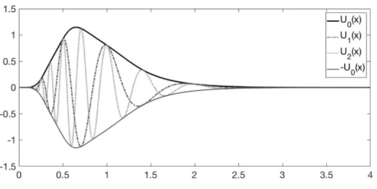
We illustrate here first the case Bpxq “ x2_{: in Figure 1, we draw the real part of}

the first eigenvectors, taken for k “ 0, 1, 2. The oscillatory behaviour will depend on the projection of the initial condition on the space generated by pUkq: it will

be stronger if the coefficients for k ‰ 0 are large compared to the projection on U0. We show two results for two different initial condition (Figure 2, Left

and Right respectively), one a peak very close to the Dirac delta in x “ 2 and the other very smooth. In both cases, the solution oscillates, as showed in Figures 3 and 4, though since the projections on X are very different (with a much higher projection coefficient on the positive eigenvector for the smooth case than for the sharp case) these oscillations take very different forms. In the second case, they are so small that for any even slightly diffusive numerical scheme they are absorbed by the diffusion, leading to a seemingly convergence towards the dominant positive eigenvector. We also see that the equation is no more regularizing: discontinuities remain asymptotically for the Heaviside case. To explore the speed of convergence in the Theorem 2 and Corollary 1, we choose Bpxq “ x3_{, take a very smooth initial condition (Figure 5 Left), with} 8

ş

0

uin

pxqxdx “ puin, U0q “ 1, for which the coefficients puin, Ukq decrease rapidly

with k, so that Rtuin is very well estimated by the series truncated for k “ 5.

We then take a refined grid with n “ 500 and N “ tn log n_{2 log 2}u “ 2241. To estimate U0, we use that _{log 2}1

t`log 2

ş

t

ups, xqe´s_{ds tends to U}

0, and take this limit value

to define Un

Figure 1: The real part for the three first eigenvectors U0, U1, U2for Bpxq “ x2.

We see the oscillatory behaviour for U1and U2.

Rtuin as pRtuinqn “ 5

ř

k“´5

puin, U_knqe2ikπlog 2tUn

k, and define the two error terms in

the discrete norm E₂n defined as E2:

Error2En 2 :“ › › › › unpt, xqe´t´ pRtuinqn › › › › 2 En 2 , Error Mean2En 2 :“ › › › › 1 log 2 t`log 2 ş t unps, xqe´sds ´ U0n › › › › 2 En 2 , (14)

where unis the numerical approximation of u. We observe several phases, which illustrate exactly the theory. First, a very fast decay of the quantity ErrorEn

2,

linked to its initial very high value since the constant C such that uin

ď CU0

is very large. Then we have a phase of exponential decay for both ErrorEn 2

and Error MeanEn

2 (the linear decay in Figure 5 Right), corresponding to a

spectral gap, as proved in [22] for the assumption of a compact support, which is satisfied here due to the truncation. Of note, this phase lasts much more for Error MeanEn

2 than for ErrorE2n, most probably due to averaging errors in the

non-oscillatory solution. The final phase is either a plateau for Error MeanEn 2

(linked to our definition of Un

0) or a quadratic increase for ErrorEn

2, which is

linked to the fact that the convergence constant in Theorem 3 depends linearly on the final time.

Discussion

We studied here the asymptotic behaviour of a non-hypocoercive case of the growth-fragmentation equation. In this case, the growth being exponential and

Figure 2: Two different initial conditions. Left: peak in x “ 2. Right: uin

pxq “ x2expp´x2

{2q.

Figure 3: Time evolution of max

xą0 upt, xqe ´t_.

Left: for the peak as initial condition. Right: for the smooth initial condition.

the division giving rise to two perfectly equal-sized offspring, the descendants of a given cell all remain in a countable set of characteristics. This results in a periodic behaviour, the solution tending to its projection on the span of the dominant eigenvectors. Despite this, we were able to adapt the proofs based on general relative entropy inequalities, which provide an explicit expression for the limit.

Our result could without effort be generalised to the conservative case, where only one of the offspring is kept at each division: in Equation (1), the term 4Bp2xqup2xq is then replaced by 2Bp2xqup2xq. The consequence is then sim-ply that the dominant eigenvalue is zero, a simple calculation shows that the dominant positive eigenvector is x U pxq, and all the study is unchanged.

Equation (1) may also be viewed as a Kolmogorov equation of a piecewise deterministic Markov process, i.e. as the equation satisfied by the expectation of the empirical measure of this process, see [14, 24]. Our study corresponds ex-actly to the case without variability in the growth rate studied in [18]. In [18], a

Figure 4: Size distribution upt, xqe´t _{at five different times (each time is in a}

different grey). Left: for the peak as initial condition. Right: for the smooth initial condition. 0 2 4 6 8 10 size 0 0.5 1 1.5 0 10 20 30 40 time 10-40 10-20 100 1020

Figure 5: Left: initial distribution (full blue line) and dominant eigenvector (doted red line), for Bpxq “ x3_{. We see that the constant such that u}in

ď U0is

very large. Right: time evolution of ErrorEn

2 (doted red line) and Error MeanEn2

(full blue line), in a log scale for the ordinates.

convergence result towards an invariant measure for the distribution of new-born cells is proved (this measure being xBpxqU pxq up to a multiplicative constant). However, this does not contradict the above study, because the convergence result concerns successive generations and not a time-asymptotics. A determin-istic equivalent corresponds to studying the behaviour of a time-average of the equation. Corollary 1 confirms that if we rescale the solution by e´t_{and average}

it over a time-period, it does converge towards U .

Our result could also easily be extended to the case where the division kernel is self similar, i.e. kpy, dxq “ 1_yk0pdx_y q, and is a sum of Dirac masses specifically

Σ is such that

DL P N˚Y t`8u, Dθ P p0, 1q, Dpp`q`PN, `ďLĂ N, 0 ă p`ă p``1@` P N, ` ď L ´ 1,

Σ “ tσ`P p0, 1q; σ`“ θp`u , pp`q0ď`ďLare setwise coprime.

This condition expresses the fact that all the descendants of a given individual evolve permanently on the same countable set of characteristic curves. The case of binary fission into two equal parts corresponds to L “ 1 and pL “ 1₂. Note

also that for the same reason, an oscillatory behaviour also happens for the coagulation equation in the case of the so-called diagonal kernel [27].

Other generalisations may also be envisaged, for instance to enriched equa-tions, or to other growth rate functions satisfying gp2xq “ 2gpxq, see [15], that is, functions of the form gpxq “ xΦplogpxqq where Φ a logp2q periodic function. An interesting future work could consist in strengthening the convergence result in Theorem 2. Indeed this result does not provide any rate of decay and the speed of convergence may depend on the initial data uin_{. A uniform}

exponential convergence would be ensured for instance by [1, Proposition C-IV.2.13], provided that one can prove that 0 is pole of A. This appears to be a difficult question, which is equivalent to the uniform stability of pTtqtě0 in XK

or to the uniform mean ergodicity of pTtqtě0in E2.

We chose to work in weighted L2 _{spaces because the theory may be}

devel-oped both very simply and elegantly in this framework, where the terms are interpreted in terms of scalar product and Fourier decomposition. The asymp-totic result of Theorem 2 could most probably be generalised to weighted L1 spaces, by considering the entropy inequality with an adequate convex func-tional. Developing a theory in terms of measure-valued solutions, in the same spirit as in [23], would also be of interest, since the equation has no regularising effect: an initial Dirac mass leads to a countable set of Dirac masses at any time.

Acknowledgments

M.D. has been supported by the ERC Starting Grant SKIPPERAD

(num-ber 306321). P.G. has been supported by the ANR project KIBORD, ANR-13-BS01-0004, funded by the French Ministry of Research. We thank Odo Diek-mann and Rainer Nagel for their very useful suggestions.

References

[1] W. Arendt, A. Grabosch, G. Greiner, U. Groh, H. P. Lotz, U. Moustakas, R. Nagel, F. Neubrander, and U. Schlotterbeck. One-parameter semi-groups of positive operators, volume 1184 of Lecture Notes in Mathematics. Springer-Verlag, Berlin, 1986.

[2] O. Arino. Some spectral properties for the asymptotic behavior of semi-groups connected to population dynamics. SIAM Rev., 34(3):445–476, 1992.

[3] D. Balagu´e, J. A. Ca˜nizo, and P. Gabriel. Fine asymptotics of profiles and relaxation to equilibrium for growth-fragmentation equations with variable drift rates. Kinet. Relat. Models, 6(2):219–243, 2013.

[4] J. Banasiak. On a non-uniqueness in fragmentation models. Math. Methods Appl. Sci., 25(7):541–556, 2002.

[5] J. Banasiak and L. Arlotti. Perturbations of positive semigroups with appli-cations. Springer Monographs in Mathematics. Springer-Verlag, London, 2006.

[6] J. Banasiak and W. Lamb. The discrete fragmentation equation: Semi-groups, compactness and asynchronous exponential growth. Kinetic Relat. Models, 5(2):223–236, 2012.

[7] J. Banasiak, K. Pich´or, and R. Rudnicki. Asynchronous exponential growth of a general structured population model. Acta Appl. Math., 119(1):149– 166, 2012.

[8] G. I. Bell. Cell growth and division: III. conditions for balanced exponential growth in a mathematical model. Biophys. J., 8(4):431–444, 1968.

[9] G. I. Bell and E. C. Anderson. Cell growth and division: I. a mathemat-ical model with applications to cell volume distributions in mammalian suspension cultures. Biophys. J., 7(4):329–351, 1967.

[10] E. Bernard and P. Gabriel. Asynchronous exponential growth of the growth-fragmentation equation with unbounded fragmentation rate. arXiv:1809.10974.

[11] J. Bertoin. The asymptotic behavior of fragmentation processes. J. Eur. Math. Soc., 5(4):395–416, 2003.

[12] J. Bertoin and A. Watson. Probabilistic aspects of critical growth-fragmentation equations. Adv. in Appl. Probab., 9 2015.

[13] M. J. C´aceres, J. A. Ca˜nizo, and S. Mischler. Rate of convergence to an asymptotic profile for the self-similar fragmentation and growth-fragmentation equations. J. Math. Pures Appl., 96(4):334–362, 2011. [14] B. Cloez. Limit theorems for some branching measure-valued processes.

Adv. in Appl. Probab., 49(2):549–580, 2017.

[15] O. Diekmann, H. Heijmans, and H. Thieme. On the stability of the cell size distribution. J. Math. Biol., 19:227–248, 1984.

[16] M. Doumic and M. Escobedo. Time asymptotics for a critical case in fragmentation and growth-fragmentation equations. Kinetic Relat. Models, 9(2):251–297, 2016.

[17] M. Doumic and P. Gabriel. Eigenelements of a general aggregation-fragmentation model. Math. Models Methods Appl. Sci., 20(05):757, 2009. [18] M. Doumic, M. Hoffmann, N. Krell, and L. Robert. Statistical estimation of a growth-fragmentation model observed on a genealogical tree. Bernoulli, 21(3):1760–1799, 2015.

[19] K.-J. Engel and R. Nagel. One-parameter Semigroups for Linear Evolution Equations. Springer-Verlag, New York, 2000.

[20] M. Escobedo, S. Mischler, and M. Rodriguez Ricard. On self-similarity and stationary problem for fragmentation and coagulation models. Ann. Inst. H. Poincar´e Anal. Non Lin´eaire, 22(1):99–125, 2005.

[21] P. Gabriel and F. Salvarani. Exponential relaxation to self-similarity for the superquadratic fragmentation equation. Appl. Math. Lett., 27:74–78, 2014.

[22] G. Greiner and R. Nagel. Growth of cell populations via one-parameter semigroups of positive operators. In Mathematics applied to science, pages 79–105. Academic Press, Boston, MA, 1988.

[23] P. Gwiazda and E. Wiedemann. Generalized entropy method for the re-newal equation with measure data. Commun. Math. Sci., 15(2):577–586, 2017.

[24] B. Haas. Asymptotic behavior of solutions of the fragmentation equation with shattering: an approach via self-similar Markov processes. Ann. Appl. Probab., 20(2):382–429, 2010.

[25] A. J. Hall and G. C. Wake. Functional-differential equations determining steady size distributions for populations of cells growing exponentially. J. Austral. Math. Soc. Ser. B, 31(4):434–453, 1990.

[26] H. Heijmans. An eigenvalue problem related to cell growth. J. Math. Anal. Appl., 111:253–280, 1985.

[27] P. Lauren¸cot, B. Niethammer, and J. J. L. Vel´azquez. Oscillatory dynamics in Smoluchowski’s coagulation equation with diagonal kernel. Kinetic Relat. Models, 11(4):933–952, 2018.

[28] P. Lauren¸cot and B. Perthame. Exponential decay for the growth-fragmentation/cell-division equation. Comm. Math. Sc., 7(2):503–510, 2009.

[29] P. Michel, S. Mischler, and B. Perthame. General entropy equations for structured population models and scattering. C. R. Math. Acad. Sci. Paris, 338(9):697–702, 2004.

[30] P. Michel, S. Mischler, and B. Perthame. General relative entropy in-equality: an illustration on growth models. J. Math. Pures Appl. (9), 84(9):1235–1260, 2005.

[31] S. Mischler and J. Scher. Spectral analysis of semigroups and growth-fragmentation equations. Ann. Inst. H. Poincar´e Anal. Non Lin´eaire, 33(3):849–898, 2016.

[32] K. Pakdaman, B. Perthame, and D. Salort. Adaptation and fatigue model for neuron networks and large time asymptotics in a nonlinear fragmenta-tion equafragmenta-tion. J. Math. Neurosci., 4(14):1–26, 2014.

[33] B. Perthame. Transport equations in biology. Frontiers in Mathematics. Birkh¨auser Verlag, Basel, 2007.

[34] B. Perthame and L. Ryzhik. Exponential decay for the fragmentation or cell-division equation. J. Differential Equations, 210(1):155–177, 2005. [35] J. Sinko and W. Streifer. A model for populations reproducing by fission.

Ecology, 52(2):330–335, 1971.

[36] C. Villani. Hypocoercivity. Mem. Amer. Math. Soc., 202(950):iv+141, 2009.

[37] A. A. Zaidi, B. van Brunt, and G. C. Wake. A model for asymmetrical cell division. Math. Biosc. Eng., 12(3):491–501, 2015.

[38] A. A. Zaidi, B. Van Brunt, and G. C. Wake. Solutions to an advanced functional partial differential equation of the pantograph type. Proc. A., 471(2179):20140947, 15, 2015.