DISCLAIMER OF QUALITY
Due to the condition of the original material, there are unavoidable
flaws in this reproduction. We have made every effort possible to
provide you with the best copy available. If you are dissatisfied with
this product and find it unusable, please contact Document Services as
soon as possible.
Thank you.
Due to the poor quality of the original document, there is
some spotting or background shading in this document.
COMMUNICATION ASPECTS OF
PARALLEL PROCESSING
Ciineyt Ozveren*
Laboratory for Information Decision. Systems
Massachusetts Institute of Technology
Cambridge, MA 02139
December 4, 1987
Abstract
Parallel processing was motivated by the need to solve very large computa-tional problems, such as the numerical solutions of partial differential equations in the context of computational fluid dynamics, structural mechanics, image processing, etc. This report surveys recent literature on parallel processing al-gorithms for mainly rings, meshes, and hypercubes. These alal-gorithms include vector, matrix computations, fixed point iterations and linear equation solvers. A group property of above topologies has also been explored in an attempt to develop tools for algorithms and performance analysis. Some special sparsity structure of the iteration dependencies has also been examined. A necessary and sufficient condition for the reducability of a dependency matrix with sparse, nonzero extended diagonals has been derived.
Work of the author supported in part by the Air Force Office of Scientific Research under Grant AFOSR-88-0032.
tational problems, such as the numerical solutions of partial differential equations
in the context of computational fluid dynamics, structural mechanics, image pro-cessing, etc. [1]. Suppose that we have a large scale computational problem and
n identical computation units, or processors, connected via some communication
network or "topology". It will be assumed that there is a relatively small number
of powerful processors (like the Intel hypercube, 128 microprocessors [71), as op-posed to many simple processors (like the Connection Machine, 65000 processors). The processors cooperate in solving the computational problem. Each works on a
different part of the problem and exchange information according to need or some schedule. The primary goal here is to minimize the total time needed to solve the
problem.
1.1
Motivation
As a motivation, let us consider the following classes of problems:
Problem 1.1 Consider a fized point problem given by the iteration:
x[k + 1] = f(x[k]) (1)
where x[k] is an N dimensional vector. Given an initial value x[O], the serial al-gorithm iterates until /(x[k]- x[k - 1])'(x[k]- x[k - 1]) < e for some given error
tolerance E. Suppose that A is a "dependency matrix", /1], for f in iteration (1), i.e. aii is nonzero if and only if fi is a function of xi. Then from a parallelization
point of view, the above problem is equivalent to the iteration:
x[k + 1] = Ax[k] (2)
A special case of Equation 1 is when x corresponds to the lexicographic ordering of variables defined on a grid where the iteration for each variable depends only on its immediate neighbors. A typical example of this is solving a partial differential equation, of say two variables, numerically by discretizing it over a two dimensional array of points and using a Jacobi type of an iteration, [14]. g*
Problem 1.2 Consider solving a set of N linear equations of N variables:
Ax = b (3)
given b and a square, invertible (for simplicity) A. A numerically sound way to solve this is by first finding a QR decomposition of A and then doing a backsubstitution to find x (see [4]). QR decompositon reduces A to an upper triangular matrix using orthogonal transformations. These are simultaneously applied to b. The modified set of equations can now be solved iteratively by first calculating xN and then using this to calculate xN-1, etc. However, this approach may be undesirable for large and sparse A since it does not make use of any sparsity structure of A. An alternative approach is to use the conjugate gradient algorithm (see [4]). This algorithm is an
iterative one that is guaranteed to terminate in N steps and executes the following in its main body:
= rklrk-/rk 2 rk (4)
pk = rk-l + PkPk-1 (5)
ak = rklrk-1/pkApk (6)
elliptic and hyperbolic equations using multigrid methods. They also consider a parallel preconditioner for the above algorithm, which is based on the Fast Fourier
Transform. This preconditioner estimates the inverse of A above and uses it to improve the convergence rate of the conjugate gradient algorithm. *e
Suppose that for each problem above, the variables in question are distributed
among some processors. Based on the following types of interconnections between
these processors, or networks:
* Ring
* Mesh
* Hypercube
which are explained in Section 2.1, this report analyzes the following standard
com-putations:
* Exchange information with another processor.
* Inner product of two vectors.
* Matrix-Vector multiplication.
* Matrix-Matrix multiplication.
* Matrix transpose.
* One to one: This is mainly due to one particular processor exchanging infor-mation with another processor.
* Broadcast (Accumulation): In this case, one processor sends the same message
to all the other processors. This comes up, for example, when the termination
of an algorithm, decided on by a designated processor, is communicated to all
the other processors. Accumulation comes up in calculating the inner product
of two vectors such that their corresponding entries are stored in the same
processor.
* Multinode Broadcast (Accumulation): In this case, all processors broadcast. For example, when a copy of a vector needs to be stored in all the processors,
each processor broadcasts the entries it stores. Multinode accumulation is
identical to multinode broadcast.
* Scatter (Gather): In this case, a particular processor sends a different message
to every other processor. For example, a designated processor distributes a
vector over all the other processors. Gather is the dual of scatter, in that a
particular processor receives different messages from every other processor.
* Multinode Scatter (Gather): This is equivalent to matrix transpose if a num-ber of rows (or columns) of a matrix are stored in each processor.
1.2
Overview and Outline
Saad and Schultz [12,131 present algorithms for the standard traffic distributions
above with no specific application in mind. Bertsekas and Tsitsiklis [1] improve
hypercubes and discuss general purpose algorithms, such as the standard
compu-tations above, and numerical solutions of elliptic and hyperbolic equations. They
present results and performance plots for the various algorithms that they
imple-mented on the Caltech and Intel hypercubes.
Unfortunately, there seems to be a lack of mathematical tools that could ease the
analysis of different algorithms by taking advantage of common features of different
classes of networks and the repetitious nature of the standard traffic distributions.
In particular, it is not clear why certain networks are easier to analyze than others.
Therefore, all the algorithms are essentially regenerated for different classes of
net-works and for different traffic distributions. I will try to improve on this by using
group theory in describing certain classes of networks.
Section 2 defines the classes of networks considered in this report, presents best
known algorithms for the standard traffic distributions and concludes by using group
theory to derive some general results. Section 3 presents algorithms for the standard
computations and the two problems discussed above. It also presents algorithms
for iterative problems where the A matrix has some "regular" sparsity structure.
Section 4 summarizes conclusions of the author and discusses possible extensions of the work surveyed in this report.
2
Results on Standard Traffic Distributions
Efficient algorithms for standard operations motivated in the previous section are
known for various classes of networks. A network is in general represented by a
graph G = (N,A) as a collection of nodes, N, and bidirectional arcs, A. An arc
(i,j) E A is assumed to represent a full-duplex link (communication can proceed
in either direction simultaneously) between the nodes i,j E N. Also, I will assume
that each link provides an error free message pipe (i.e. it is assumed that if an error
occurs, it is detected and corrected in a negligible amount of time. This is not a
very realistic assumption in general. However it is consistent with the assumptions
of the papers surveyed and the consequences will be briefly discussed in Section
4). Note that the arcs constitute a measure of distance for the set of nodes, i.e.
d(i,j) = 1 if (i,j) E A and in general the length of the shortest path between i and j. A path is specified as a sequence of neighboring nodes (distance 1 apart).
Suppose that a traffic distribution is specified in terms of messages of length
li,j to be sent from node i to node j for various pairs of nodes, that are not
nec-essarily neighbors. In a communication network, a major problem, given a traffic
distribution, is how to schedule these messages such that total communication time
is minimized. This is termed routing. Routing is typically solved locally (at each
node) since otherwise communication overhead to gather traffic information and
then distribute routing results would be very excessive. This in general is a hard problem. For parallel processing algorithms considered in this report, traffic
distri-bution is known a priori and it is assumed that the network belongs to a class which
is "regular" in some sense. This enables one to precisely specify the path followed
by each message and makes the timing analysis much easier. Different types of
delays at the intermediate nodes.
* Connectivity: Provides a measure for the number of "alternate" paths con-necting a pair of nodes. Node (arc) connectivity is defined as the minimum
number of nodes (arcs) that must be deleted before the network becomes
disconnected. If a network has arc connectivity k, then there are at least
k parallel paths, i.e. paths with no arcs in common, between any pair of
nodes (max flow - min cut theorem [8]). This is important for reliability
pur-poses. Also, the communication between any pair of nodes can be parallelized
by splitting the message into several parts and sending each on a different
path. If there is no other traffic crossing these paths and the overhead cost
for communication is low (not a valid assumption in general) then the total
communication time for this message is reduced by a factor of k.
* Flexibility: Ability to efficiently run a broad variety of algorithms. For
exam-ple, an algorithm may be most suitable for a particular type of network. If
this network can be imbedded in another network (in a way that preserves the
neighborhood structure), but perhaps not vice versa, then the latter network
is more flexible than the former since it can run algorithms for both.
2.1
Classes of Networks
()-1'
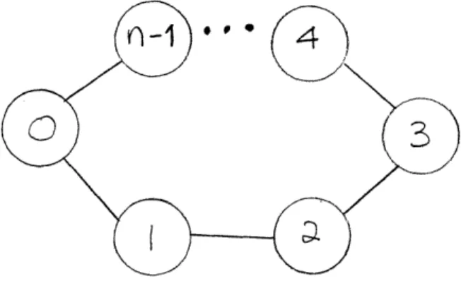
Figure 1: n Node Ring
2.1.1 Rings
A ring with n nodes, is illustrated in Figure 1. It has diameter n/2, and arc
connectivity 2. It will be assumed that the nodes are indexed consecutively by
integers, as in the figure.
2.1.2 Mesh
An n node d dimensional mesh is a d dimensional array of n = nln 2... nd nodes
({ni} is a positive, nonincreasing sequence of integers). It is assumed that the nodes
are indexed as d-tuples (zl,... , xd) where each xi is an integer modulo ni. Only the
immediate neigbors are connected, i.e. two nodes are connected only if their indices
differ by one only in one coordinate. A wraparound mesh is one where two nodes
are connected only if their indices differ by one modulo ni only in some coordinate
i. This report only considers wraparound meshes due to their symmetric structure.
An example of such a mesh is illustrated in Figure 2. A wraparound mesh has
diameter (n1 + ... + nd)/2 and arc connectivity 2d.
Let us now consider imbedding a ring into a mesh with the same number of
neigh-Figure 2: A Two Dimensional 5 x 3 Wraparound Mesh
borhood structure, i.e. neighbors are mapped to neighbors. For simplicity, let us
consider two dimensional meshes. First recognize each, say, row of the mesh as a
ring. Then, join the second row with the first to form another ring (for example,
see Figure 3). To do this, break a link in the first row, and its counterpart in the second row. Join the nodes at the end points of these liks. Next, join the third row
with the second, in the same fashion. Note that here, a link different than the one
picked in the previous case should be used. Proceed likewise with the other rings.
At the third step, the link picked at the first step can be used, etc. Therefore,
we never run out of links to pick. This can be extended to higher dimensions in
a straightforward way. Also, using above approach, conditions can be derived for
imbedding a ring in a mesh with more nodes.
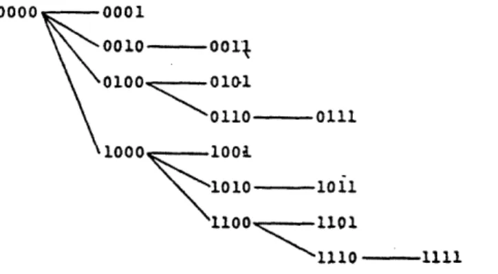
2.1.3 Hypercube
Let Hd represent a d-dimensional hypercube, see for example Figure 4. It has 2n nodes. Assume that these nodes are indexed by binary numbers of length d bits,
B. Then two nodes are connected if and only if their indices differ by one bit. The
l ' ~v l~ ..
F--: iUaRi i ax
XOO 1o0 0110 '11
iioi
Figure 4: Hypercube, d -= 4
is termed the Hamming distance and it can be calculated using the exclusive OR
function (XOR). XOR of two bits is 0 if they are equal and 1 if different. Let a
and b be two nodes in a hypercube, then aXORb is defined as the binary number
obtained by XOR of corresponding entries of a and b. Hamming distance, dh(a, b), is the number of l's in aXORb.
Any ring with an even number of nodes can be imbedded in a hypercube of
equal or more nodes. First of all, note that a d dimensional hypercube consists of two d-1 dimensional hypercubes with corresponding nodes connected. Let us first
consider rings with 2d nodes. Clearly, we can perform this imbedding when d = 2.
Suppose we can do it for some d. For d + 1 take two d dimensional hypercubes
and the corresponding link in the other. Connect the corresponding nodes of the
two hypercubes at either side of these links. We thus have an imbedding in the
d + 1 dimensional hypercube (see Figure 5). This corresponds to traversing the
nodes in one hypercube in the reverse direction of the other and generates the so
called Binary Reflected Gray Codes [1,11,7]. In general, when the ring has an even
number of nodes, r, it can be imbedded in a hypercube with equal or more nodes
by joining the corresponding r/2 node portions of the rings at lower dimension. If
a ring has an odd number of nodes then it cannot be imbedded in a hypercube
since a hypercube has no cycles (i.e. no paths that finish at the nodes they start)
with an odd number of nodes, [11]. A mesh with even ni can be imbedded in a hypercube of dimension flog nll + .-- + Flog ndl (all logs are base 2). Using the
imbeddings of a ring each column can be imbedded in a hypercube of dimension [log nil. Corresponding nodes of these hypercubes form a hypercube of dimension
[log n2l. Thus, they may be combined by n2 node rings. Higher dimensions are
imbedded similarly.
For all the network classes above I assume that communication can be carried
out simultaneously on all links of a node in both directions. In [7], it is implicitly
assumed that a node can transmit on only one link and receive on another at any
given time. Although in practice it seems to be possible to transmit and receive
on more than one link at a time, if not all links, I will consider both extremes
for hypercubes. I refer to them as type 1 and type d. Bertsekas and Tsitsiklis [1]
0000 0001 \\ 0010 ---001'-0100 0101 10 0110 0111 1010 1011 1110 -1111
Figure 6: Tree Used for Broadcasting in a Hypercupe of Dimension d
2.1.4 Trees
A tree is any connected network with no cycles. Note that a tree with n nodes has
exactly n- 1 links (see for example Figure 6). Thus all trees have arc connectivity
1. The tree in Figure 6 has diameter 7. In general, trees are not very practical as
physical networks due to their low connectivity. However, they are useful
concep-tually since they prevent data duplication in broadcast situations. Specifically, a
spanning tree of a network, which is a subgraph of the network that includes all the
nodes but has no cycles, is important (for example, Figure 6 is a spanning tree of a
4 dimensional hypercube).
2.1.5 Fully Connected
Examples of these are shared memory, crossbar switch (just like a phone system switch board), broadcast bus (every node is tapped on to a bus and only one can transmit at a time). I will not consider these networks since, as the number of nodes increases, shared memory and the switch network become impractical to
implement, and time available for each node to transmit on a broadcast bus goes
2.2
Standard Traffic Distributions
I will present algorithms for some standard traffic distributions on the network
classes discussed above. I will assume that all messages are of unit length, and
in most cases, present results in terms of the order of time needed in units of the
transmission time of a unit length message. This will be denoted by O(e). If f is
O(g) but not o(g) then f will be termed O.(g), i.e. strictly order g. If the best
possible algorithm for a problem is known to be 0. (g) and we have an algorithm that
is O(g) then that algorithm will be termed efficient. It is assumed that transmitting
a message of length 1 over a link takes c + lv units of time. Here c represents fixed
costs, such as the propagation delay, and v represents variable costs, such as the
transmission time.
2.2.1 One to one
In this case, one node sends a message to another node. The easiest way to do this
for the rings is just to send the message along the shortest path, which requires time
(c + Iv)s where s is the length of the shortest path. Note that this may be bounded
by (c + lv)n/2. A better approach is to send part of the message through the
alternate longer path, specifically a portion proportional to the length of the paths. In this case, total transmission time may be bounded by (c + lv)n/4. In [12], the
message is divided into smaller messages and pipelined through the shortest path.
This yields an equation for the total transmission time as a function of the number
_ ,-r.
.0-* ·. . · A B A B
Figure 7: Parallel Paths on a Mesh
Yet another way is to send these smaller messages through both paths in a pipelined
fashion. In general, one to one ring algorithms are O,(n).
For a mesh, it is shown in [12] that there are four parallel paths between any two nodes a, b of a two dimensional grid with wraparound (recall that we already
know this fact from the Min-Cut Max Flow Theorem). In particular (see Figure 7),
* If a and b are aligned on the grid, then these paths can be chosen to be of
length d(a, b) + 2 each.
* If a and b are aligned, in either the horizontal or vertical direction, but are not neighbors, then four paths can be chosen to be of length d(a, b) + 4.
* If a and b are neighbors, then four paths can be chosen to be of length d(a, b) +
6=7.
Thus, as in rings, the message could be divided into smaller messages, and can be
sent through these parallel paths in a pipelined fashion. In general, one to one grid
algorithms are 08(nl).
For hypercubes, it is shown in [13] that there are d parallel paths between any
differing bit from the right and propagating to left. The second path is chosen by
starting from the second differing bit, circulating and finally finishing with the first
differing bit from the right. In this fashion, i parallel paths can be chosen. For the
rest, first flip a bit that is identical in a and b. Then correct all the differing bits,
there are i + 1 of them now, in any order but leave the previously correct bit to the
last. Since there are d - i bits common to both a and b, d - i additional paths can
be chosen with length i + 2 each. For type d, the message can be divided up and
pipelined along these parallel paths. The resulting algorithm is O0(d). For type 1,
pipelining is not useful but the message could still be divided up into pieces. Each
piece should be sent to a different neighboring node one by one. It is slightly better
if the nodes that are further away are started from. The algorithm is still O.(d) but the coefficient is doubled.
For all the above networks, pipelining is a final touch of optimization, otherwise
they are of the same order.
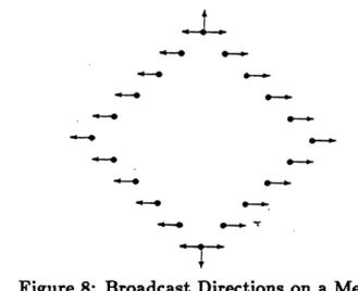
2.2.2 Broadcast
In this case, a node sends the same message to all other links.
For rings, all nodes have two links and the best strategy would be to transmit
on both sides of the broadcasting node. Here, the algorithm is O,(n). In [121, an
algorithm of the same order of transmission time is given for the pipelined case.
For meshes, a similar strategy could be used. The message should be transmitted
Figure 8: Broadcast Directions on a Mesh
direction of broadcast at each level so that no message is duplicated (see Figure 8 for illustration). Details of this algorithm and a variation based on splitting the message into a horizontal and vertical part are given in [12]. In both cases, the algorithm is lower bounded by the maximum ni, i.e. it is
O,(nl).
For hypercubes, algorithms for this in [13,1,7] are all based on the same idea. There is no difference between type 1 and type d. The property that Hd consisists of two Hd-i with corresponding nodes connected, is used. The broadcast node sends its message to the adjacent H-ld. Now, we have two parallel broadcast problems on two Hld-1. Proceeding iteratively, the message is broadcast in d steps. An alternative representation of this algorithm is the tree in Figure 6. This tree is illustrated for node 0. The corresponding tree for any other node a can be generated by performing an XOR of a and each node on the tree. Note that this is a permutation of the tree such that the root is node a and the neigborhood structure is preserved. This is formally proved in Section 2.3.
The dual of the broadcast problem is accumulation, which can be executed in the same amount of time by reversing the steps of above algorithms.
the ring. Each node receives a message from one direction and transmits it at the
next step on the other direction. This requires Os(n) time, but additional savings,
by a factor of 2 can be made by broadcasting in both directions simultaneously.
Note that this is efficient since every node can receive two messages at every step
and there is a total of n messages.
For meshes, the best algorithm in [12] is based on two passes. at the first step,
a multinode broadcast is performed on each, say, horizontal ring of the mesh. Note
that after the first pass, each node has n1 messages corresponding to its horizontal
counterparts. These messages are then broadcast along vertical rings, requiring a
total of O, (n) time. Note that this algorithm is efficient since each node can receive
4 messages at a time and there is a total of n messages.
For hypercubes of type 1, multinode broadcast can be done using the vector shift
algorithm of [7]. A ring with 2" nodes is imbedded in a d dimensional hypercube. Multinode broadcast can be equivalently formulated as storing a vector of length
n, whose elements are originally assigned to the processors in a one to one fashion,
in each processor. The elements of this vector are shifted one by one along the
ring until all processors receive the vector elements. This algorithm is O,(n) and efficient since each node can receive at most one message at a time and there is a
total of n messages. For type d, there are various multinode broadcast algorithms
in [13] and only one of them is efficient (Optimal Total Exchange Algorithm). It is
0 (n/d), or Os(n/ log n), and efficient since there are d links from each node and a
each step, to scan the messages they currently hold to decide on which messages
to send to their neighbors at that step. This requires processing time by the host
processor and, depending on the particular architecture, it may take a considerable
amount of time. A better algorithm is presented in Section 2.3.
2.2.4 Scatter, Gather
In the case of gather, one node receives a different message from every other node.
Note that gather is a special case of multinode broadcast. Furthermore, every node
has to receive n different messages. Thus, the algorithm for each network has a
lower bound of n divided by the number of links from each node in that network.
The multinode broadcast algorithms achieve this bound. Therefore, they are also
efficient for gather ([13] has a gather algorithm for hypercubes which is not even
efficient). Note also that a dual of gather is scatter. Efficient algorithms for scatter
can be achieved by reversing the traffic streams of a gather algorithm.
2.2.5 Multinode Scatter or Matrix Transpose
In this case, every node sends a different message to every other node. For rings
if we let each node scatter in turn, we have an O(n2) algorithm. Note that the
messages corresponding to one node traverse n/2 links on the average. Since there
are n nodes with n messages each and a total of n links, each link transmits an
average of n2/2 messages. Therefore, the above algorithm is efficient.
For meshes (the algorithm in [12] is wrong since for example, a processor on the
diagonal never sends any messages to the processors in its row), say of dimension 2,
first at each row we have a multinode scatter of messages destined for each column
messages corresponding one node traverse 0s(nl + n2) links on the average. Since
there n nodes with n messages each and a total of 2n links, the above algorithm is
efficient. For higher dimensional meshes, the corresponding algorithm will have the
same order.
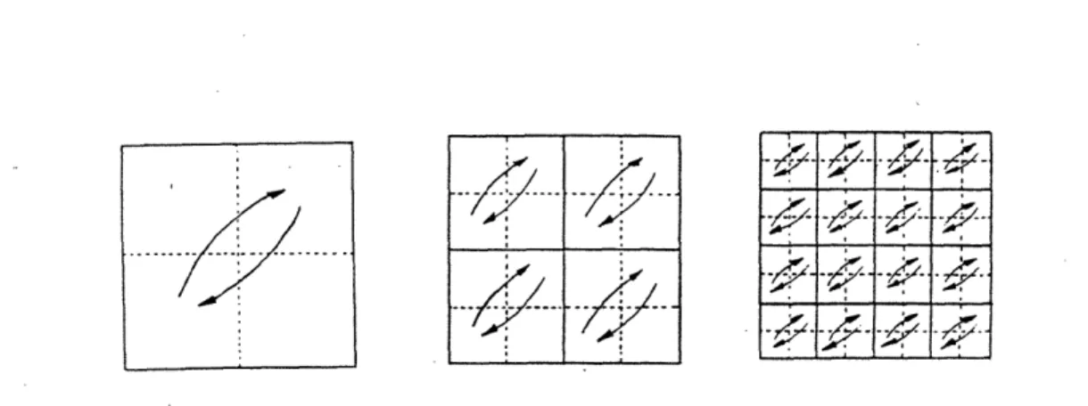
For hypercubes of type 1, the algorithm in [7] uses a matrix transpose
inter-pretation. Suppose that we have an n x n matrix whose rows are distributed over
Hd (n = 2d). First divide the matrix into four blocks and exchange off diagonal
blocks. This corresponds to exchanging messages between corresponding nodes of
two Hd-l. Then divide each block into four sub-blocks and apply the above step
to each block (see Figure 9). Iterating until we have 1 x 1 sub-blocks completes
the algorithm. Note that at step i of the algorithm, 2d-i2i- 1 = 2d-1 messages are exchanged between each pair of nodes. Since there are d steps, the algorithm
is O(d2d) = O(dn). For multinode scatter, each node transmits O,(n) messages,
where each message goes through O,(d) nodes on the average. Since each node
can transmit one message at a time and there are n nodes, the above algorithm is efficient. For hypercubes of type d, consider the following algorithm in [1]: This
algorithm has two parts. First, a multinode scatter is performed in each Hd-l and
in parallel each node sends the data for the other hypercube to the corresponding
node (2d-1 messages). Then, a multinode scatter is performed on each Hdl for these messages. It can be shown inductively that this algorithm is 08 (n). Note
that this algorithm can also be generated from the above algorithm for type 1.
Figure 9: Matrix Transpose Algorithm for Hypercube Dimension 3, Type 1
Ring Mesh Hypercube Type 1 Type d One to One n n7 d d Broadcast n nl d d Multinode Broadcast n n n n/d Scatter n n n n/d Multinode Scatter n2 nln dn n
Table 1: Orders of algorithms for standard operations on regular networks
the first part). Then, off-diagonal blocks are transposed (this is the second part).
Note that this algorithm is also efficient.
The results presented in this section are summarized in Table 1.
2.3
Group Properties of Some Networks
It turns out that the nodes of rings, meshes and hypercubes can be indexed such
that the set of indices is a group under some operation. Morover, neighborhood
structure and the shortest path between any pair of nodes can be described in a
e*a=a for all a E G 2. For every a E G there is a b in G with
b * a=e (Then b is the inverse of a, denoted by a-1.)
Moreover, a group is abelian if * commutes. **
For rings, let Z, be the set of integers modulo n. Then Z, is an abelian group
under addition modulo n, call this *,. The shortest path distance on a ring dr(a, b)
for any a, b E Zn is given by min(a *, b-', a-l *, b).
For meshes, suppose that the nodes are indexed consecutively along each
di-mension by Z x ..*** x Z,, = M. Let a, b E M and a = (al,...ad), b = (bl,...bd). Then M is an abelian group under addition, c = a *m b, such that ci = as *i bi or
ci = a, + bi (mod ni). Then, the shortest path distance between any two points a, bE M is:
d
dm(a, b) = min(a, *i b-1, ai- *i bi)
i=1
For hypercubes, define a function gh : B --i Z as the number of 1's in a binary
number. Note that B is a group under bit by bit XOR, *h, and the shortest path
distance, which is the same as the Hamming distance, is given by dh(a, b) = gh(a*hb).
Note that the inverse of any element in B is itself.
Consider a network such that the indices of nodes form an abelian group G
nodes a, b E G satisfies d(c * a, c * b) = d(a, b) for all c e G. Specifically, it is
important that arcs map to arcs. Note that this is satisfied by rings, meshes and
hypercubes. Suppose that we have an algorithm for broadcast from node e (the node
whose index is the identity element in the group). In particular, this algorithm is
specified as a set of distinct directed arcs Ai that transmit a message at step i
of the algorithm. Let (a,b) E Ai and consider c * (a,b) = (c * a, c * b). Since
d(c * a, c * b) = d(a, b) = 1, c * (a, b) is also an arc. Moreover, since broadcast from e
sends the message from e to all other nodes and operating on these nodes by some
node c is just a permuation of the nodes such that e maps to c, transmitting over
the arcs c * Ai at step i achieves broadcasting from node c. Therefore, it is sufficient
to construct a broadcast algorithm from one node. The rest can be generated from this.
A straightforward approach to multinode broadcast is to let each node broadcast
simultaneously using a broadcast algorithm. Recall that for the broadcast from
node e, its message is transmitted over the arcs Ai at step i. This algorithm may
be generalized to multinode broadcast such that at step i, the set of directed arcs
Ai,a = a * Ai (* of each element of Ai by a) transmit the message corresponding to
node a. Let (x, y) be an arc and ri(x, y) be the number of Ai,a that contain (x,y),
i.e. r,(x, y) is the number of messages that need to be sent on arc (x, y) at step i.
Thus step i takes
rmzi - max ri(x, y) (z,y)EAi,,. aEG
units of time. The sequence of sets Ai should be picked such that total completion
time of the algorithm, ]i r,,,a,i is minimized. I claim the following:
Proposition 2.2 Given Ai, let (x,y) E Ai and
Proof: First of all, let (z, w) E R,(x,y) and a = y * w-I (note that a E G. Then,
(a * z, a * w) = (y * w- 1
* z, y) = (x, y) (using commutativity). On the other hand,
Let (x, y) E Ai,a for some a. Then, (x, y) = (a * z, a * w) for some, but only one,
(z, w) E Ai. We have, x * y-1 = a * z * w- 1 * a- 1 = z * - 1.
Note that we can apply the above result to all Ai,a individually. But also,
R(a * x, a * y) = a* R(x, y). Thus,
rmaz~i = max ri (x,y)
(zy)EAi
i.e. we only need to look at the arcs for node e, and we have:
rmz,,i = max
IRi(x,y)l
(9)(zy)EAi
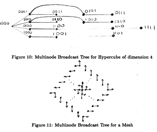
In short, we wish minimize the number of arcs that carry traffic in the same direction at the same step. For hypercubes, these arcs correspond to arcs that flip the same bit. Note that the tree in Figure 6 would lead to a multinode broadcast in O(n) steps. Conceptually, we should be able to generate a tree with about n/d levels and at most d arcs at each level such that all arcs at the same level flip a different bit. I propose the following: Consider a tree generated by d major steps and some minor steps in each major step. At major step i, all nodes with labels that have exactly i bits equal to 1 are connected to the other elements of the tree generated upto step i. In each minor step corresponding to step i, d of these nodes are connected to any previously generated element of the tree such that each arc corresponds to a different bit flip. The tree is generated when finally node Id (a
001 i r QO t Otst
Figure 10: Multinode Broadcast Tree for Hypercube of dimension 4
This algorithm is O~(n/d) and efficient.for a mesh, as in Figure 11, that produces an efficient multinode Broadcast Tree for Hypercube of dimension 4
(compare to Figure 8). Note that this approach could also be applied to multinoded
scatter problems or any other problem such that the transmissions for all the nodes
can be generated from the transmissions for one node using the group operation.
lems.
3.1
Vector Computations
Let us first consider computation of the inner product of two vectors. This is
important for calculating the termination condition of a relaxation algorithm (for
example checking to see if the norm of the error vector is small enough) and also
constitutes a basis for matrix-vector multiplications. Suppose that two given vectors
of length n each are distributed over n processors in a way that corresponding entries
of each vector reside in the same processor. Let each processor calculate that portion
of the inner product corresponding to the entries it holds. It then sends its result
to another processor which adds it to its own computation and sends the result to
another processor etc. The result is finally summed up at a designated processor.
Thus, we have an accumulation (of the designated processor) problem. In relaxation
algorithms, when this inner product is the norm of the error vector, if this norm is
small enough then the designated processor sends a termination message to all the other processors. This is a broadcast problem.
Next let us consider a problem of shifting a vector by a certain amount. This is
particularly interesting and important (since it constitutes a basis for matrix-vector
multiplication, etc.) for type 1 hypercubes. In this case, ordering of distribution
over the processors of the hypercube is important. In particular, assuming that the vector has n elements, each consequtive entry of the vector will be distributed
according the embedding of a ring into the hypercube (as generated using Binary
Reflected Gray Codes). As a result of this imbedding, nodes that have logical
distance 2k on the ring, for some k, have physical distance 2 on the hypercube
[1]. The algorithm in [7] uses this to construct a logical hierarchy of the ring in
the hypercube (see Figure 12). The important issue here is that at level k of this
hierarchy, there are 2k parallel cycles corresponding to connections of each node with
the nodes of logical distance 2k . Thus, it takes two units of time to shift a vector by
2k elements, for any k > 1 and one unit of time for k = 1. Consider shifting a vector
arbitrarily by some amount s > 0. We can assume that s < 2dsince shifting by 2d is the same as not shifting at all. Also, we can assume that s < 2d- 1 since shifting in one direction by s is the same as shifting in the other direction by 2d - s and when
s > 2dwe could save on the number of shifts by shifting in the other direction. Let us take the binary expansion of s, i.e. let s = bd-2 ... bo. In [71, they achieve this
shift by a combination of shifts depending on which bits of s are set. Since shifting
by one requires one step and the rest require two steps each, they have an algorithm
that works in 0(2(d - 2) + 1) time in the worst case. Note that for a shift by 7,
this requires shifting by 4, shifting by 2 and finally shifting by 1. However, it would
take less time if this vector was first shifted by 8 and then shifted in the reverse
direction by 1. To generalize this, one needs to solve a shortest path problem. It
can be shown that any shift can be done in at most d steps, an improvement by a factor of two (see Appendix A).
3.2
Matrix Computations
Let us first consider how to store a matrix in n processors. Let us assume that the
Level O \N 0110 010 0011 01i0 - . .1 .1010 .. cl1 3-0 11 Level2 X
·..
1
Figure 12: The logical hierarchies of rings in a 16-node hypercube and the commu-nication channels used to implement them.
* By rows: Store each row in a processor.
* By columns: Store each column in a processor.
* By diagonals: The matrix A is converted into diagonal form D (see Figure 13) and D is stored by columns.
Note that conversion from storage by rows to by columns and vice versa requires
multinode scatter. For each case above, we have the following algorithms:
* Suppose that the matrix is stored by rows and each processor has a copy of
the vector. Then in O(n) computation time the product is calculated and
entry p of the resulting vector is stored in processor p. If we are running a
relaxation algorithm, we need to redistribute the entries of the vector to all
the processors. Thus we do a multinode broadcast.
· Suppose that the matrix is stored by columns and processor p has entry p of the vector. Each vector multiplies the column and the vector entry it stores.
Then in O(n) computation time, we have n vectors that are distributed over
processors and need to be summed up. Since we want processor p to have entry p of the resulting vector, each processor needs to gather corresponding
entry from every other processor. Here we have multinode gather. Note that
alternatively, the entry may be added up at the intermediate processors. In
this case, we have a multinode accumulation which would make the total
cost of running the algorithm same as the storage by rows. However, as
each processor accumulates its message, intermediate nodes need to add the
different messages destined for the same node and form a new message. Thus,
A 20 21 22 23 24 25 4051 02 13 24 35 30 31 32 33 34 35 30 41 52 03 14 25
40 41 42 43 44 45 20 31 42 53 04 15
50 51 52 53 54 55 10 21 32 43 54 05
Figure 13: Conversion of A to Diagonal Form D
result in longer running time than the previous one, but perhaps the same order of magnitude.
* Suppose that the matrix is stored by diagonals and processor p has entry p of the vector. Then an algorithm can be constructed that consists of n successive shifts by one, and O(n) computation before each shift (see [7]). They argue in [7] that this storage is portable in the sense that it does not bias A towards either row or column storage. This seems to be a reasonable argument for hypercubes of type 1. However, if the same storage is used for hypercubes of type d, corresponding calculation would take time by a factor of d larger than
that of either row or column storage.
When multiplying two matrices A and B, the most favourable case is when A is stored by rows and B is stored by columns. The algorithm would be to perform
n successive matrix-vector multiplications. The resulting matrix is stored by rows,..,
3.3
Fixed Point Problems with Sparse A
Fixed point problems can simply be solved by a repeated application of the
matrix-vector product considered above. However, for sparse A, this approach may not
be very efficient. Some forms of sparsity structure are examined below. When
necessary, applications to hypercubes of type d are used for illustration. In what
follows, it is assumed that A is a square matrix of dimension N x N where N = mn and n is the number of processors as usual.
3.3.1 Banded
Suppose that A is distributed among the processors in blocks of m rows, and
sim-ilarly, x is distributed in blocks of m elements. Moreover, corresponding blocks
of A and x reside in the same processor (for example, first m rows of A and first
m elements of x are stored in the same processor) and the consecutive blocks are
stored in neighboring processors (for example, for the hypercube, the imbedding of
a ring into the hypercube would be used). To define what is meant by banded let
us first consider the notion (of [71) of an extended diagonal. An extended diagonal
p of A is the set of entries {a/j such that j - i = p or i- j = n - p}. The
sym-metric counterpart of this diagonal is the set of entries {ai, such that i - j = p or
j - i = n - p}. When an extended diagonal is nonzero, it will be assumed that
its symmetric counterpart is also nonzero. A matrix A will be termed banded with
width b if extended diagonals 1, ... b and their symmetric counterparts are nonzero
and the rest of the matrix is zero. It will be assumed that b is a multiple of m,
say b = rm. Then the corresponding fixed point iteration can be computed by r
consequtive shifts in both directions. Each shift consists of transmitting m elements
previous section if roughly, r < n/d.
3.3.2 Mesh
In certain cases, such as the 5-point discretization of a partial differential equation
using the Jacobi method (see [14]), the "dependency graph" (i.e. the graph
gener-ated by modelling each variable as a node, and defining an undirected arc between
nodes i and j for all nonzero aij of the dependency matrix) may be a wraparound
mesh. Distribution of variables among n processors is modelled, in [7], as a
prob-lem of dividing a rectangle into n regions with minimum perimeter to area ratio.
They assume that the mesh is N1 x N2 = n1p1 x n2p2 and the number of available processors is nxn2. In this case, they argue that, to minimize communication, the
mesh should be divided into squares with P1P2 points each, if possible (otherwise
near square rectangles). Each processor is assigned one of these rectangles. The
dependency graph for the processors is then a wraparound mesh itself. At each iteration of the fixed point computation, each processor exchanges data with its
horizontal and vertical neighbors. Recall that wraparound mesh consists of rings
in horizontal and vertical directions. Thus, a shift by one in each direction of all
horizontal and vertical grids may be done in parallel. This algorithm takes roughly
0(V/p-) communication time (on the appropriate mesh or type d hypercube).
In 9-point discretizations, the dependency graph includes diagonal connections
(see Figure 14). Suppose that this graph is N x N and n = p2for some integer p that
Figure 14: 4 x 4 Mesh Corresponding to a 9-Point Discretization
sap
i
SicpFigure 15: Decomposition of Diagonal Exchange
In this case, we have a similar p x p graph for which data corresponding to r points
need to be exchanged on the vertical and horizontal directions, and 1 point on the
diagonal directions, at each iteration. The data exchange can be performed on a
p x p mesh of processors in two steps. Suppose that diagonal exchange is divided into
its horizontal and vertical components as in Figure 15. At the first step, horizontal
and vertical exchange takes place. This also covers the first components (horizontal
or vertical) of the diagonal exchange. At the second step, the second components
the above where r, = (i + 1)k and N is a multiple of k (see Figure 17), is
undesir-able when the matrix-vector multiplication method above is applied. However, this
problem can be divided into k disjoint problems, each indexed by i E {0,-. , k - 1}.
Problem i corresponds to iteration of variables {i, k + i,... , N/k - 1 + i}. For
the general case, group theory is useful. Let G be the group of integers modulo N
with group operation of addition modulo N. In general, decomposition into disjoint
problems relies on finding Rp = [ro] * [rl * ... [rp-1], where [a] denotes the set of all
powers of a, which is a subgroup of G, [10], and [a] * [b] = {ai * b,, for some i and j}.
The disjoint problems are Rp and its cosets, [101. I first make the following claim:
Proposition 3.1 Rp = [ro] * [rl] * ..' * [rpl] = [qp] where qp = gcd(ro, ... , rp_-, N).
Proof: I prove this inductively. First, [ro] = [q1]: Since rO = q; for some integer s,
[ro] C [ql]. Let a E [ql] then a = qh for some h. Note that h E G. Since s, above, and N are relatively prime and s G G, [s] = G and thus for any h 6 G, there exists
some w E G such that h = sW. Therefore, a = q"' = ro' E [ro].
Suppose, R, = [qpl, then Rp+l = [qpl * [rp] = [qp] * [s] where s = gcd(rp, N). On
the other hand, N = qp+l(qp/qp+i)(s/qp+l)w for some w. Thus,
,Rp+l - [N/(s/qp+l)J * [N/wi * [NI(qplqp+l)] * [N/w] = [Nl(s/qp+l)] * [N(qpl/qp+l)] * [N/w]
00
Note that there are exactly qp cosets of [qp]. To summarize, we have the following:
Proposition 3.2 For a fixed point problem, or a matrix-vector multiplication
prob-lem, where A is structured as above, the problem can be divided into qp disjoint problems (i.e. A is reducible to a block diagonal form) and moreover, the indices of the variables that belong to each problem are given by [qpl and its cosets. *.
If the number of available processors, n, is less than or equal to qp then one
or more subproblems can be assigned to each processor appropriately. (If n < qp,
depending on the problem, it may be better to distribute some of the subproblems
over all the processors to balance the computation load on the processors.) If n = qp,
then there is no communication cost, and the computation executes n times faster
than the serial one. If n > qp, say n = mqp for simplicity, then m processors could
be assigned to each problem. In this case, if possible, either band or grid structure
could be exploited as above or a straightforward matrix-vector multiplication type
of an algorithm could be applied.
In general, comparison of a parallelized fixed point iteration to its serial version
is hard because the performance is strongly coupled to the sparsity structure of
A and how it is exploited. In the case of linear iterations with dense A, a serial
algorithm takes O(m2n2) computation steps. For hypercubes of type d, parallel
ver-sion takes O(mn/d) communication steps and O(m2) computation steps. Typically, computation is much faster than communication (for example for-Intel hypercube
[7]). Thus, for moderate m, communication will dominate computation and paral-lelization will be beneficial when unit communication cost to unit computation cost
is roughly less than md/n. For large m, computation will dominate and
Figure 16: Scattered Extended Diagonals (entries nonzero only along the lines in-dicated)
L k4 k k.
Figure 17: A Special Case of Scattered Extended Diagonals
[7] is the communication penalty, which is defined as the ratio of communication time per iteration to computation time per iteration. In this case, communication penalty is O(n/dm) which approaches zero as m increases implying that processors are fully utilized.
3.4
Linear Equation Solvers
3.4.1 Orthogonalization
Let us first consider the QR decomposition (Q is not constructed explicitly, but
the same transformations are applied to b). Suppose that A is mn x mn and stored by rows. In this case the dimension of the matrix being worked on
de-creases with each step. To preserve effective use of each processor, suppose rows
p,p+ n, ... ,p + (m - 1)n are stored at processor p. At each step, one column is
or-thogonalized. At step i, each processor first orthogonalizes that piece of the current
column it stores, and this takes O((m - i/n)(mn - i)) computation time. Then the
remaining part of the column (one entry per processor) need to be orthogonalized.
However, the resulting transformation must to be applied to the rest of the rows.
This can be achieved either using Modified Gram-Schmidt or a series of Givens transformations, [4], over a tree (such as the tree in Figure 6). In either case, the
required communication time is O(d(mn - i)) and the computation time is also
O(d(mn - i)). Summing this over mn steps, we get O(dm2n2) communication time
and O(m3
n2) computation time. Backsubstitution takes O(mn) time. The serial
version of this algorithm takes O(m3n3) computation steps. Thus parallelization is
favourable when unit communication time to computation time ratio is roughly less
than mn/d. Communication penalty is O(d/(m + n)) which approaches zero as m increases.
3.4.2 Conjugate Gradient
In this section, I calculate the execution time of Equations (4-8) of the first section. All vectors and the matrix A, mn x mnn, are assumed to be distributed by rows. The
a copy of pk), and thus takes O(mn/d) communication time. If A is sparse, this
may of course be further improved, if possible, using the approach of Section 3.3.
Equations (7) and (8) are immediate after Equation (6). Thus each iteration takes
a total of O(mn/d) communication time and O(m2n) computation time. In the
serial version each iteration takes O(m2n2) computation steps. Therefore, if the
communication to computation ratio is roughly less than mnd, it will be preferable
to parallelize. Note that the iterative version is faster, by a factor of O(d2), than the
QR decomposition approach above even in the worst case convergence of mn steps.
Furthermore, the iterative version can be made faster if A is sparse. Note also that
4
Conclusions and Further Questions
This report has surveyed part of the recent literature on the communication aspects
of parallel processing. Among the topologies considered, hypercubes have the best
properties in terms of diameter, connectivity, and flexibility. For the standard
oper-ations, efficient algorithms are known for the popular topologies. From a practical
point of view, matrix vector product seems to be the most important computation.
This computation, for dense A, is rather straightforward. However, exploiting the
sparsity structure of A is a hard problem in general.
As a tool for exploring structures of "regular topologies" and analysing timing
properties of algorithms for these topologies, the application of group theory was
proposed and carried out to some extent. An interesting result was presented on the
reduceability of a sparse matrix with nonzero extended diagonals. One could argue that such matrices may not be found in practice since if the matrix is reducible, then
this perhaps can be recognized at the modelling stage. However, the matrix may
be "almost reducible" in the sense that appropriate extended diagonals are O(e) for
some small E. This would correspond to weakly coupled subproblems of the large
scale problem. Then a processor can be assigned to each subproblem and a two time
scale update could be carried out, i.e. variables corresponding to each subproblem
are updated frequently with respect to other variables in that subproblem and are
updated at a slower rate (perhaps bounded by communication time) with respect
to the variables in other subproblems.
The algorithms considered in-this report were essentially synchronous. Although
the processors operate asynchronously in principle, each processor waits for all the variables necessary for an update before performing that update (local
particular processor the message is destined for. Since other processors will wait for the results of this update in their next update, execution of the algorithm would be
delayed arbitrarily. A potentially more robust approach is the use of asynchronous
algorithms, [1]. Typically, in this case, each processor performs the updates as
many times as possible regardless of whether it has the most recent values of the
variables in other processors. A major drawback of these algorithms is that their
convergence properties are much harder to analyze.
Another aspect of reliability is the extent of damage caused by a failure, such
as a link or node crash, on the overall communication properties of the network.
For example, when a link crashes, a natural remedy would be to reroute the packet
through an alternate path. However, there could conceivably be other packets using
the links on this path, and they will be delayed due to the rerouted packet. For
example, for the algorithms considered in this report, the precise scheduling of the
messages would be disrupted and communication time estimates would not be valid
anymore. Note that the nodes are generally aware of the current traffic distribution.
The network may use this to its advantage by implementing a different (perhaps
pre-calculated) schedule.
I believe that the recent developments on the control of Discrete Event Dynamic
Systems, [2,3,5,6,9], may be used to address robustness problems. In particular, the
work of Ramadge and Wonham 19], Lin and Wonham [6] and Cieslak et al. [2]
could be helpful in designing a local control that reacts to link failures. The work of
the times at which the messages are introduced into the network, on the queue sizes.
Finally, perturbation analysis of Ho [5] might be useful in analyzing the effects of
path problem and shows that this can be done in at most d steps. Consider the following scalar linear system:
x[k + 1] = 2x[k] + u[k]
where u[k] is restricted to 1 (forward shift), 0 (no shift), -1 (reverse shift). Let x
be the desired amount of shift and consider a minimum energy control problem to
reach x in the above system in some number of steps. Let us plot the state space
of this system and formulate this as a shortest path problem where absolute values
of u[iJ are the arc lengths. Figure 18 illustrates this for a 32 node ring. Note that
initial input of -1 is omitted due to the symmetric nature of the state space and we
do not need to consider any states larger than 16 since we can equivalently achieve
it by reversing the shifts. The numbers in squares beside the states are the shortest
path lengths. For example, a shift of 7 can be achieved by a shortest path through
0, 1, 2, 4, 7, with a corresponding length of 2, and input string 1, 0, 0, -1 which
corresponds to a forward shift by 23 = 8 and a reverse shift by 1. The graph for
larger rings can be generated by bulding on this ring. A ring with 2d nodes will
have a graph with d- 1 levels. At each level, maximum shortest path length of
an even numbered state is the same as maximum shortest path length of an odd
numbered state in the previous level. On the other hand, maximum shortest path length of an odd numbered state is one plus maximum shortest path length of an
even numbered state in the previous level. It can be shown inductively that at level
0
-l
©
-Figure 18: State Space for a 32 Node Ring
is even, and (k + 1)/2 for all states if k is odd. Recall that shifts that are nozero
powers of 2 take two steps. Also, note that exactly one shift of an odd numbered
node will be a single step shift and all shifts of even numbered nodes take two steps.
Therefore, it follows that arbitrary shifts require at most d steps for hierarchical
rings with 2d nodes on a hypercube.
B
Multinode Broadcast Tree for Hypercubes
To prove the existence and the timing properties of a multinode broadcast tree for
hypercubes as derived in Section 2.3, I will use the equivalence classes defined in
Note that in all the equivalance classes, there is an element with a one in the first
bit and other elements are shifts of this element. Given an element of A(d, i), if we
change a one entry of this number to a zero, the resulting number is an element of
A(d, i-1). Therefore, all elements of an equivalance class of A(d, i) can be connected
to elements of A(d, i-1) in a way that each connection flips a different bit. To prove
that the number of minor steps in a major step is bounded by (d)/d+ 1, it suffices to
prove that at most one equivalance class of A(d, i) has less than d elements (others
have exactly d elements).
Proposition B.1 There are exactly
(i)l
equivalance classes of A(d,i).Proof: Let us first prove that there is at most one equivalance class with less than
d elements in it. Let a E A(d, i) and j be the smallest integer such that a = Sia.
Suppose j < d and without loss of generality, assume that a has a one as the
rightmost bit. Denote the positions of ones in a by integers modulo d such that e is
the position of the rightmost bit. By the property of cyclic shift, ones are located
at [j], that is, at j,2j,... etc. By the proof of Proposition 3.1, [j] = [p] where
p = gcd(n,j). Also, p' = e and thus pi = d. Therefore, given i, p is unique and
furthermore, it exists if and only if i divides d.
Using the fact that A(d, i) has (d) elements, we achieve the desired result. **
Note that the tree in Figure 10 can be improved by filling the gaps (see Figure
19). However, if d is prime, then all equivalance classes (except for the one
corre-sponding to i = d) have d elements and improvement is not possible. Note that
loll I toOl OQ
\I il 011) O l1 ol
I I~ 0, i" Ol~ 9 }rIO0 dc 000 ) 1 0 I ,O ,N 0to ; fo
[2] R. Cieslak, C. Desclaux, A. Fawaz, P. Variaya, "Modeling and Control of
Dis-crete Event Systems", Proceedings of CDC, Dec 1986.
[3] G. Cohen, D. Dubois, J.P. Quadrat, M. Viot, "A Linear System Theoretic
View of Discrete Event Process", Proceedings of CDC, Dec 1983.
[4] G. H. Golub, C. F. Van Loan, Matrix Computations, Johns Hopkins University
Press, 1983.
[5] Y. Ho, "Performance Evaluation and Perturbation Analysis of Discrete Event
Dynamic Systems", IEEE Trans. on Automatic Control July 1987.
[6] F. Lin, W.M. Wonham, "Decentralized Supervisory Control of Discrete Event
Systems", University of Toronto Paper, July 1986.
[7] 0. A. McBryan, E. F. Van de Velde, "Hypercube Algorithms and Implemen-tations", Siam J. Sci. Stat. Comput., March 1987.
[8] C. H. Papadimitriou, K. Steiglitz, Combinatorial Optimization, Prentice-Hall,
Inc., 1982.
[9] P.J. Ramadge, W.M. Wonham, "Supervisory -Control of a Class of Discrete
Event Processes", University of Toronto Paper, Nov 1985.
[11] Y. Saad, M. H. Schultz, "Topological Properties of the Hypercube", Yale
Uni-versity Report, February 1985.
[12] Y. Saad, M. H. Schultz, "Data Communication in Parallel Architectures", Yale
University Report, March 1986.
[13] Y. Saad, M. H. Schultz, "Data Communication in Hypercubes", Yale University
Report, August 1987.
[14] G. D. Smith, Numerical Solution of Partial Differential Equations: Finite