Resolution limit of taylor dispersion: an exact theoretical study

Resolution Limit of Taylor Dispersion: An Exact Theoretical Study

Patricia Taladriz-Blanco,

†

Barbara Rothen-Rutishauser,

†

Alke Petri-Fink,

†,‡

and Sandor Balog

*

,†

†_{Adolphe Merkle Institute, University of Fribourg, Chemin des Verdiers 4, 1700 Fribourg, Switzerland} ‡_{Chemistry Department, University of Fribourg, Chemin du Musée 9, 1700 Fribourg, Switzerland}

*

S Supporting Information

ABSTRACT: Taylor dispersion is a microfluidic analytical

technique with a high dynamic range and therefore is suited well to measuring the hydrodynamic radius of small molecules, proteins, supramolecular complexes, macromolecules, nanoparticles and their self-assembly. Here we calculate an unaddressed yet fundamental property: the limit of resolution, which is defined as the smallest change in the hydrodynamic radius that Taylor dispersion can resolve accurately and precisely. Using concepts of probability theory and inferential statistics, we present a comprehensive theoretical approach, addressing uniform and polydisperise particle systems, which involve either model-based or numerical analyses. We find a straightforward scaling relationship in which the

resolution limit is linearly proportional to the optical-extinction-weighted average hydrodynamic radius of the particle systems.

T

aylor dispersion, being akin to dynamic light scattering, enables measuring the hydrodynamic radius of particle systems but is less liable to a moderate presence of sample impurities,1,2and therefore there is a considerable interest from bionanotechnology, including pharmacology and toxicology in the technique.3−24

The question we address in this Letter is straightforward and addresses an elementary analytical property that has never been studied before: What is the resolution limit of Taylor dispersion? By definition, the resolution limit is the smallest change, let it be either increment or decrement in the hydrodynamic radius r, that Taylor dispersion is able to measure accurately and precisely. In other words, it is the smallest δr value where the chance of failing to resolve the difference between r and r ± δr is practically zero. To justify the subject, it is indisputable that a fine limit of resolution is essential to evidence and quantify subtle changes. For instance, characterizing the hydrodynamic radius marks the stages of protein denaturation,25 polymer degradation,26 solvent-de-pendent conformation,27 and dissolution of ingested nano-particles.28Taylor dispersion is linear and time-invariant,29and accordingly, it is possible to resolve the distribution of the hydrodynamic radius of polydisperse and multimodal systems by inverting (“deconvoluting”) Gaussian superpositions.10,15 Accordingly, better measurements pave the way for a deeper understating of, e.g., the interaction of proteins with surfactants30 and lipids,31 biological activity of particulate nanomaterials,32,33etc., which all arguably result in safer food ingredients, more natural personal hygiene products,34 and novel therapeutics superior to current standards.35

Taylor dispersion combines the phenomenon of optical extinction, translational self-diffusion, and sheer-induced dispersion in a steady Poiseuilleflow.36−38An initially narrow

band of the injected analyte broadens along the capillary upon traveling with the flow, and the extent of band-broadening contains accurate information about the translational self-diffusion coefficient of the dispersed material. The so-called taylorgram is the temporal record of the band broadening, and the concentration is usually measured via UV−vis spectrosco-py. If the detector response is linear, and the volume of the injected sample and the volume of detection are both negligibly small compared to the capillary volume, the taylorgram of a uniform material of hydrodynamic radius r dispersed in a cylindrical channel is36−38

A t A t ( ) 0 1 e (t t0) /t 2 πκ = − − κ (1)

where A0 is the amplitude of the absorbance, quantified by particle type, particle concentration, and capillary radius Y,κ = rπηY2_{/(2 k}

BT), T is temperature,η is viscosity of the fluid, kBis the Boltzmann constant, and t0= x/v is the so-called residence time defined by the distance between detection and injection points and the mean velocity of the flow (v). The temporal mean and variance of the absorbance profile are t0+κ/2 and (t0+κ)κ/2. When the residence time t0is much larger thanκ,

eq 1is essentially Gaussian, and one can accurately measure the hydrodynamic radius, by determining κ from the absorbance profile

r k T Y 2 B 2 πη κ = (2)

http://doc.rero.ch

Published in "Analytical Chemistry 92(1): 561–566, 2020"

which should be cited to refer to this work.

Taylor dispersion is subject to errors that erode the reliability of determining r. Errors are classified as either systematic or random, and the impact of the latter is referred to as precision, which is usually quantified either as standard deviation or relative standard deviation of a set of measure-ments. Precision may be considered at three levels: repeatability, intermediate precision, and reproducibility. It has been shown recently that the variables ineq 2, the width-parameterκ, temperature T, viscosity η, and capillary radius Y, are directly relevant to the precision of the Taylor dispersion, and the precision may be expressed via the expectable errors of the corresponding variables39

r r T T Y Y 2 2 2 2 2 L N MMM \ ^ ]]] L N MMM \ ^ ]]] L N MMM M \ ^ ]]] ] L N MMM \ ^ ]]] κ κ η η Δ = Δ + Δ + Δ + Δ (3)

Here we are building on this result, while considering that the fundamental aspect of experimentation is simple: one performs and analyzes n = 1,2,3,...n measurements independ-ently, under identical conditions, and usually reports the average and standard deviation of the n results. From a statistical point of view, a set of such results is a random sample, with a sample size of n, drawn from the population whose parameters are r and Δr (eqs 2 and 3).38 The population is the ensemble of the realizable measurement, and owing to random errors, the population is heterogeneous. In other words, if one measures n times, which in technical terms means sampling with replacement, where one draws randomly and independently n elements of the population, one tends to obtain n different results owing to sample-to-sample variations. According to the central limit theorem, the sampling distribution of the mean approximates a normal distribution, regardless of the shape of the distribution describing the population. If r and Δr are the population parameters of a normal distribution, the distribution of the sample mean rs is practically already normal at small sample sizes (n < 10)

g r r n n r , 2 e n r r(s ) /22 r2 L N MMMM \ ^ ]]]] _π Δ _≅ Δ − − Δ (4)

with a mean equal to r, and with a standard deviation equal to

r/ n

Δ . The latter is frequently referred to as the standard error of the mean.

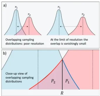
The expectable precision of determining the hydrodynamic radius is therefore Δr/ n. As a result, the sampling distributions corresponding to two sets of measurements of two hydrodynamic radii that are close to each other may overlap (Figure 1). This may be the case when r1< r2with r2/ r1≅ 1, i.e., when the difference between r1and r2is small.

When the overlap is considerable, the chance of evidencing the difference between r2 and r1 is low. This is because the chance of ambiguous results increases with the area defined by the overlap, and to be able to quantify the difference between r2and r1, the overlap of the two sampling distributions must be vanishingly small. Otherwise, the chance that the two sample means falling in the area of the overlap becomes high enough. According to eq 4, to decrease the area of the overlap, one must (a) either increase the distance between r1 and r2, (b) increase the precision of measuring r1and r2(i.e., decreaseΔr,

eq 3), and (c) increase the sample size n (number of measurements). Therefore, the minimum distance (i.e., the difference in size) that can be resolved between r1and r2 is

defined by the sample size and the precision attainable in the measurements.

This qualitative picture is quantified next, and we show that the overlap has a clear probabilistic meaning, which is then applied to give a quantitative and clearly defined answer to the limit of resolution of Taylor dispersion. As illustrated inFigure 1b, the area of the overlap is the sum of two components: P1+ P2where P g r r n r n R r r , d 1 2 1 2 erf ( ) 2 R 1 1 1 1 1 1 1 L N MMM MM \ ^ ]]] ]] L N MMM MM \ ^ ]]] ]]

∫

= Δ = − − Δ ∞ (5) P g r r n r n R r r , d 1 2 1 2 erf ( ) 2 R 2 2 2 2 2 2 2 L N MMM MM \ ^ ]]] ]] L N MMM MM \ ^ ]]] ]]

∫

= Δ = + − Δ −∞ (6)

Each component represents a cumulative probability: P1is the cumulative probability that the mean value of the n1 measurements of the hydrodynamic radius r1 falls over the intersection point R, and P2is the cumulative probability that the mean value of the n2measurements of the hydrodynamic radius r2 falls below the intersection point R. Therefore, the area of the overlap quantifies the probability P = P1+ P2that the mean of either or both of the measurements falls on a “wrong” interval of the sampling distributions. Naturally, if this probability is small, the chance of evidencing the difference between r1and r2is high.

The intersection point r1< R < r2can be found by solving the equation

Figure 1. Concept of determining the limit of resolution based on the sampling distribution of the mean (eq 4). The sampling distributions corresponding to two sets of measurements of two hydrodynamic radii r1and r2may overlap when r1and r2are close enough to one another. If the overlap is considerable, the chance of evidencing the difference between the two is low (a). This is significant, because the chance of ambiguous results, where either R < rs(1) or rs(2) < R or rs(2) < R < rs(1) increases with the area of the overlap (b). To be able to discern the difference between r1and r2with a high certainty, the overlap of the two sampling distributions must be vanishingly small.

g r r n g r r n , , 1 1 1 2 2 2 L N MMM MM \ ^ ]]] ]] L N MMM MM \ ^ ]]] ]] Δ = Δ (7)

By following some basic algebraic steps, a rearranged form gives a simple quadratic equation

n x r r n x r r Z ( ) 2 ( ) 2 2 2 2 22 1 12 12 1 − Δ − − Δ = (8) where Z1 ln

( )

r n_{r n} 1 2 2 1

= Δ_Δ , and the nontrivial solution provides two roots R n r r r r Z n r r n r n r ( ) 2 2 12 2 1 2 1 1 2 2 12 1 22 = Δ ± Δ Δ ∓ Δ Δ − Δ (9) where Z2 = n2(n1(r1 − r2)2 + 2Z1Δr12) − 2Z1n1Δr22. The solution we need is the one that is larger than r1but smaller than r2, i.e., r1< R < r2.

While eq 9 is a general solution, it may be simplified considerably by considering a special case. First, the sample size is commonly kept symmetric in experimental practice, i.e., n1 = n2, and second, according to eq 3, near to the limit of resolutionΔr2≅ Δr1because r2/r1≅ 1. By considering these two aspects, we obtain that R≅ (r1+ r2)/2, and inserting them

into eqs 5 and 6, the area of the overlap is expressed in a

straightforward manner P P P n r r r 1 erf ( ) 8 1 2 2 1 L N MMM M \ ^ ]]] ] = + ≅ − − Δ (10)

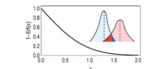
where n = n1= n2is the number of measurements and Δr = Δr1≅ Δr2is the precision of the measurements determining r2 and r1. The function f(x) = 1− erf(x) is shown inFigure 2.

As can be seen, f(x) is a monotone decreasing function that asymptotically approaches zero. In other words, there is a definite relationship between x and P: if x keeps increasing, P keeps decreasing, and the probability of obtaining ambiguous results eventually becomes vanishingly small. The inverse of this relationship is also true: when P is small, x and thus r2− r1 must be also small. Accordingly, the smaller P, the higher the probability that the difference between r2and r1is discerned and quantified from the recorded taylorgrams.

Therefore, based on eq 10, we can quantify the limit of resolution with a probabilistic exactness: Letδr be the smallest value where the odds in favor of resolving r and r +δr are not smaller than a million to one, that is, the probability of obtaining ambiguous results is 10−6

r r

n δ = Δφ

(11)

where φ ≅ 9.78 when P = 10−6. If one is less cautious and willing to accept a higher risk of obtaining ambiguous measurements, the value of P may be increased, and accordinglyδr may be smaller. For example, φ ≅ 6.58 when P = 10−3.

It is important to emphasize that according toeqs 5−11, the limit of resolution is not a universal but a rather supple parameter. It is in fact limited by the design of the experiments and the quality of the related analysis, because it is a function of (1) the probability of obtaining ambiguous results, (2) the number of measurements we are willing or able to collect and analyze, and (3) the precision one is willing (and able) to achieve in these measurements. For example, it matters whether the width parameterκ of the taylorgram is estimated by a nonlinear regression of eq 1 or by a direct numerical integration of the taylorgram itself, for the attainable precision ofΔκ will not be identical.16,39Furthermore, given thatΔr is a function of r,δr becomes also a function of r, and it is easy to show viaeq 3that by using a typical Taylor dispersion system, including typical instrument and experimental parameters, the limit of resolution is proportional the hydrodynamic radius:Δr ∝ r.

We showed previously that by using unconstrained non-linear least-squares fit to estimate the width parameter of a taylorgram of uniform particles, Δκ can be expressed as a function of four parameters:Δ =κ zκB+1t0C Dτ SNE, where z = 2.42 is a dimensionless constant, κ the value defined by the uniform hydrodynamic radius of the particles, t0 residence time,τ the temporal resolution of the taylorgram, and SN the signal-to-noise ratio. The exponents are =−0.24, C = −0.26, D = 0.5, and E =−1.16

Nonuniform particle systems, including polydispersity and multimodality, are however frequent, and their taylorgrams are analyzed in terms of temporal moments such as mean and variance to determine the optical-extinction-weighted average radius.6,12,20,23,40,41This approach involves numerical integra-tion, and noise affects the attainable precision differently than it affects model-based nonlinear regression.39 The residence time and width parameter are determined through the temporal mean (M) and temporal variance (V), and it was shown elsewhere20,23 that in the case of Rayleigh particle systems, where optical absorption and scattering are power functions of the particle radius (i.e., optical absorption coefficient at a given wavelength of a particle is proportional to its volume), the apparent hydrodynamic radius determined by Taylor dispersion isr_poly=rÙm+1/rØm, where rØm is the mth raw moment of the size distribution of the particle system:

rm P r r( ) mdr

0

Ø

∫

≡ ∞ · . Accordingly, for particles system whose optical extinction is dominated by, e.g., absorption:

rpoly r r4/ 3 × ×

= . Thus, in the case of size polydispersity: M≅ t0 + 1/2κpolyand V≅ 1/2 κpoly· (t0+κpoly), where the apparent width parameter isκpoly= rpolyπηY2_{/(2 kBT). When t0≫ κpoly,} M≅ t0and V≅ t0· κpoly/2, and thus

V M 2 poly κ ≅ (12)

and the corresponding relative uncertainty is

Figure 2. f(x) = 1 − erf(x) function describingeq 10. When f(x) is vanishingly small, the probability of obtaining ambiguous results P is also vanishingly small, i.e., the difference between r1and r2is surely expected to be evidenced.

M V poly poly 2 M2 2 V2 2 L N MMM MMM \ ^ ]]] ]]] κ κ σ σ Δ ≅ + (13)

where σM2 _{and σV}2 _{describe the uncertainty, owing to the} presence of noise, of determining the temporal mean and temporal variance of the taylogram via numerical integration. To calculate σM2 and σV2 is not trivial.39 Briefly, when the signal-to-noise ratio is not too low (i.e., the peak of the taylorgram is clearly recognizable: SN > 2), the experimentally recorded taylorgram may be decomposed into two terms, A_ϵ= A +ϵ, where ϵ represents additive noise. The origin of ϵ is the shot noise,23 and its probability density function p(ϵ) is practically Gaussian. It is easy to show that p(ϵ) is practically stationary in time when the peak absorbance is not too high (i.e., A(t0) < 0.1), which means that the variance of p(ϵ) is practically constant along the taylorgram. The value ofϵ varies randomly along the taylorgram with a zero mean ϵ̅ = 0 and variance ϵ − ϵ = ϵ2 2 2. The noise in a taylorgram is uncorrelated, that is ϵ ϵ = ϵ_{i j} 2δ_ij, where δij is the Kronecker delta. The overline denotes ensemble average:

p( ) d

∫

ϵ̅ = ϵ ϵ ϵ −∞ ∞ (14) and p( ) d 2

∫

2 ϵ = ϵ ϵ ϵ −∞ ∞ (15)

Following the definition of the signal-to noise ratio of a taylorgram,23it is not difficult to show that ϵ ≅2 A t( )/SN0

The temporal moments of a taylorgram calculated as a normalized temporal average on the closed interval capped by t_aand tb, and is defined as

t A t t A t t A t t ( ) ( ) d ( ) d w t t w t t a b a b

∫

∫

⟨ _ϵ ⟩ = ϵ ϵ ₍₁₆₎

where w = 1 or 2, taand tbenclose the peak of the taylorgram and are chosen symmetrically around the center of the peak. In experimental practice, a taylorgram is recorded with discrete time points, and thus the integration of such real-valued function becomes a summation (Riemann sum), e.g.:

A t( ) dt A t( ) t t i k i 1 a b

∫

_ϵ ≅τ

∑

= ϵ (17)

whereτ is the temporal resolution, i.e., t1= ta, t2= t1+τ, tj= t1 + (j− 1)τ, and tb= t1+ kτ, and k ≫ 1. Accordingly,

M t A t A t ( ) ( ) i k i i in i 1 1 τ τ ≅ ∑ ∑= ϵ = ϵ (18) and V t A t A t M ( ) ( ) i k i i i k i 1 2 1 2 τ τ ≅ ∑ ∑ − = ϵ = ϵ (19)

In the absence of noise, the precision and accuracy are perfect, and determining the true values of M, V andκpolyis completely assured. Given the noise, however, both M and V may vary from taylorgram to taylorgram, and accordingly, there

is uncertainty, and thusσM2> 0,σV2> 0 andΔκpoly> 0. Their expected values are calculated via ensemble averaging over the noise distribution M̅ =

∫

Mp( ) dϵ ϵ −∞ ∞ (20) V̅ =

∫

Vp( ) dϵ ϵ −∞ ∞ (21) M M M p( ) d M M2 2 2

∫

2 2 σ = − ̅ = ϵ ϵ − ̅ −∞ ∞ (22) V V V p( ) d V V2 2 2

∫

2 2 σ = − ̅ = ϵ ϵ − ̅ −∞ ∞ (23)

We could not evaluate these equations, most likely owing to singularities in these improper integrals and thus cannot present general analytical forms. Nonetheless, we found excellent approximative solutions when considering not too high noise levels, i.e., where the peak of the taylorgram is clearly recognizable, or in other words, the signal-to-noise ratio is not vanishing. First, let us define three new variables:

t A t( ) i k i i 1 α = ∑τ _{= ϵ} , _ik 1t A ti ( )i 2 β= ∑τ _{= ϵ} , andγ= ∑τ k_i=1A tϵ( )i . Consequently, M =α/γ and V = β/γ − (α/γ)2.α, β, and γ are correlated random variables, and the uncertainties in M and V may be expressed as42 M M 2 Cov( , ) M2 2 2 2 2 L N MMM \ ^ ]]] L N MMM M \ ^ ]]] ] σ α σ γ σ α γ ≅ ∂ ∂ α + ∂∂ γ + (24) and M M M

2 Cov( , ) 2 Cov( , ) 2 Cov( , )

V2 2 2 2 2 2 2 L N MMM \ ^ ]]] L N MMM M \ ^ ]]] ] L N MMM M \ ^ ]]] ] σ α σ β σ γ σ α γ α β β γ ≅ ∂ ∂ + ∂∂ + ∂∂ + + + α β γ (25)

The partial derivatives are to be evaluated at α̅, β̅ and γ̅.

Equations 24 and 25 can be evaluated analytically, and

therefore, we are still able to describe the uncertainty of numerical integration. For example, γ̅ = ∫−∞∞ γp(ϵ) dϵ = τ∫−∞∞ ∑i = 1k A(ti)p(ϵ) dϵ + τ∫−∞∞ ∑i = 1k ϵ(ti)p(ϵ) dϵ. The first term is the area under the taylorgram, and the second term vanishes because the mean of the additive noise is zero. We could evaluate similarly the other terms, and the results are

t A t( ) i k i i 1

∑

α_{̅ =}τ = (26) t A t( ) i k i i 1 2

∑

β̅ =τ = (27) A t( ) i k i 1

∑

γ_{̅ =}τ = (28) t i k i 2 2 N2 1 2

∑

σ_α = τ σ = (29) t i k i 2 2 N2 1 4

∑

σ_β =τ σ = (30)

http://doc.rero.ch

k 2 2 N2 σ_γ =τ σ (31) t Cov( , ) i k i 2 N2 1

∑

α γ =τ σ = (32) t Cov( , ) i k i 2 N2 1 3

∑

α β = τ σ = (33) t Cov( , ) i k i 2 N2 1 2

∑

β γ =τ σ = (34) whereσ = ϵ ≅N2 2 ( ( )/SN)A t0 2, M̅ ≅ α̅/γ̅ and V̅ ≅ β̅/γ̅ − (α̅/

γ̅)2_{. Accordingly, the resolution in determining the} hydro-dynamic radius via numerical integration can be evaluated via

eqs 12−35. One frequently combines the analyses of two

detection windows to determine the hydrodynamic radius11,12

V t V t M t M t 2 ( ) ( ) ( ) ( ) poly 2 1 2 1 κ = − − (35)

The related uncertainty is

t M t M t t M t M t t V t V t t V t V t ( ) ( ( ) ( )) ( ) ( ( ) ( )) ( ) ( ( ) ( )) ( ) ( ( ) ( )) poly poly 2 M2 2 2 1 2 M2 1 2 1 2 V2 2 2 1 2 V2 1 2 1 2 L N MMM MMM \ ^ ]]] ]]] κ κ σ σ σ σ Δ ≅ − + − + − + − (36)

When it comes to numerical integration, the uncertainty is increasing with the level of noise (σN) and with the length of the integration interval (tb− ta,eq 16). This is because ineqs 29−34 t 1 t t t t 2( ) 1 2 ( ) i k i 1 a b b2 a2

∑

= + + _τ − = (37) t 1 t t t t t t 2( ) 6( ) 1 3 ( ) i k i 1 2 a2 b2 b a b3 a3

∑

= + + τ − + _τ − = (38) t 1 t t t t t t 2( ) 4( ) 1 4 ( ) i k i 1 3 a3 b3 b2 a2 b4 a4

∑

= + + τ − + _τ − = (39) t t t t t t t t t 1 2( ) 30( ) 3( ) 1 5 ( ) i k i 1 4 a4 b4 3 a b b3 a3 b5 a5

∑

τ τ τ = + + − + − + − = (40)

Equations 37−40mean that the uncertainty of determining

the width and center of a taylorgram increases with the residence time (t0≅ (ta + tb)/2) and with the length of the integration intervals (tb− ta). It is worth pointing out that the uncertainty resulting from numerical integration is always inferior to that of resulting from suitable modelfitting.

To summarize, the hydrodynamic radius is a fundamental physical property, for it can indicate the onset of even minute changes in the properties of a particle dispersion, let it be natural or engineered of origin. By using concepts of probability theory and inferential statistics, we showed here

that the limit of resolution of Taylor dispersion is inherently defined by the precision attained in the given sets of measurements, and the limit of resolution ultimately scales withr/ n, where n is the number of measurements used to determine the mean value.

To demonstrate some aspects of our findings, we present two complete studies in theSupporting Information. Thefirst one is a brief theoretical study that addresses a special case: uniform particles and model fitting (The ultimate resolution limit of Taylor dispersion for uniform particle systems,Figure SI 1). Our goal was to point out that the resolution limit of optimal“noise-limited” Taylor dispersion experiments may be outstanding, which offers a performance competitive to well-established and widely used techniques, such as dynamic light scattering, fluorescence correlation spectroscopy, particle tracking analysis, and small-angle X-ray and neutron scattering. The second one is an experimental study that addresses a highly polydisperse particle system (The stability and hydro-dynamic radius of citrate-capped silver nanoparticles in water,

Figures SI 2−8). Our goal was to demonstrate how the theory

developed in this Letter may be used to design, analyze, and interpret fully realistic scenarios of Taylor dispersion experi-ments.

■

ASSOCIATED CONTENT

*

S Supporting Information

The Supporting Information is available free of charge at

https://pubs.acs.org/doi/10.1021/acs.analchem.9b03837.

Two complete studies: ultimate resolution limit of Taylor dispersion for uniform particle systems and stability and hydrodynamic radius of citrate-capped silver nanoparticles in water (PDF)

■

AUTHOR INFORMATION Corresponding Author *E-mail:sandor.balog@unifr.ch. ORCID Patricia Taladriz-Blanco: 0000-0002-2469-9704 Alke Petri-Fink:0000-0003-3952-7849 Sandor Balog:0000-0002-4847-9845 Author Contributions

S.B. conceived the idea, developed the theoretical description, and wrote the manuscript through contributions of the coauthors. S.B. and P.T.-B. designed the experimental study. P.T.-B. synthesized the particles, performed the UV−vis, the TEM, and the Taylor dispersion experiments. S.B. and P.T.-B. analyzed the experimental evidence. A.P.-F. and B.R.-R. supervised P.T.-B.

Notes

The authors declare no competingfinancial interest.

■

ACKNOWLEDGMENTS

The authors are grateful for the financial support of the Adolphe Merkle Foundation and the University of Fribourg. This work also benefitted from support (<50%) of the Swiss National Science Foundation through the National Center of Competence in Research Bio-Inspired Materials.

■

REFERENCES

(1) Hawe, A.; Hulse, W. L.; Jiskoot, W.; Forbes, R. T. Pharm. Res. 2011, 28, 2302−2310.

(2) Urban, D. A.; Milosevic, A. M.; Bossert, D.; Crippa, F.; Moore, T. L.; Geers, C.; Balog, S.; Rothen-Rutishauser, B.; Petri-Fink, A. Colloid and Interface Science Communications 2018, 22, 29−33.

(3) Bello, M. S.; Rezzonico, R.; Righetti, P. G. Science 1994, 266, 773−776.

(4) Belongia, B. M.; Baygents, J. C. J. Colloid Interface Sci. 1997, 195, 19−31.

(5) Wuelfing, W. P.; Templeton, A. C.; Hicks, J. F.; Murray, R. W. Anal. Chem. 1999, 71, 4069−4074.

(6) Cottet, H.; Biron, J.-P.; Martin, M. Anal. Chem. 2007, 79, 9066− 9073.

(7) d’Orlyé, F.; Varenne, A.; Gareil, P. Journal of Chromatography A 2008, 1204, 226−232.

(8) Le Saux, T.; Cottet, H. Anal. Chem. 2008, 80, 1829−1832. (9) Medina, C.; Santos-Martinez, M. J.; Radomski, A.; Corrigan, O. I.; Radomski, M. W. Br. J. Pharmacol. 2007, 150, 552−558.

(10) Cottet, H.; Biron, J.-P.; Cipelletti, L.; Matmour, R.; Martin, M. Anal. Chem. 2010, 82, 1793−1802.

(11) Hulse, W.; Forbes, R. Int. J. Pharm. 2011, 416, 394−397. (12) Chamieh, J.; Oukacine, F.; Cottet, H. J. Chromatogr A 2012, 1235, 174−177.

(13) Cipelletti, L.; Biron, J.-P.; Martin, M.; Cottet, H. Anal. Chem. 2014, 86, 6471−6478.

(14) Jensen, S. S.; Jensen, H.; Cornett, C.; Møller, E. H.; Østergaard, J. J. Pharm. Biomed. Anal. 2014, 92, 203−210.

(15) Cipelletti, L.; Biron, J.-P.; Martin, M.; Cottet, H. Anal. Chem. 2015, 87, 8489−8496.

(16) Lavoisier, A.; Schlaeppi, J.-M. mAbs 2015, 7, 77−83. (17) Oukacine, F.; Morel, A.; Desvignes, I.; Cottet, H. J. Chromatogr A 2015, 1426, 220−225.

(18) Pyell, U.; Jalil, A. H.; Urban, D. A.; Pfeiffer, C.; Pelaz, B.; Parak, W. J. J. Colloid Interface Sci. 2015, 457, 131−140.

(19) Høgstedt, U. B.; Schwach, G.; van de Weert, M.; Østergaard, J. Eur. J. Pharm. Sci. 2016, 93, 21−28.

(20) Balog, S.; Urban, D. A.; Milosevic, A. M.; Crippa, F.; Rothen-Rutishauser, B.; Petri-Fink, A. J. Nanopart. Res. 2017, 19, 287.

(21) Fichtner, A.; Jalil, A.; Pyell, U. Langmuir 2017, 33, 2325−2339. (22) Zaman, H.; Bright, A. G.; Adams, K.; Goodall, D. M.; Forbes, R. T. Int. J. Pharm. 2017, 522, 98−109.

(23) Balog, S. Anal. Chem. 2018, 90, 4258−4262.

(24) Oukacine, F.; Gèze, A.; Choisnard, L.; Putaux, J.-L.; Stahl, J.-P.; Peyrin, E. Anal. Chem. 2018, 90, 2493−2500.

(25) Jelińska, A.; Zagożdżon, A.; Górecki, M.; Wisniewska, A.; Frelek, J.; Holyst, R. PLoS One 2017, 12, No. e0175838.

(26) Chamieh, J.; Biron, J. P.; Cipelletti, L.; Cottet, H. Biomacromolecules 2015, 16, 3945−3951.

(27) Jin, X.; Leclercq, L.; Sisavath, N.; Cottet, H. Macromolecules 2014, 47, 5320−5327.

(28) Bove, P.; Malvindi, M. A.; Kote, S. S.; Bertorelli, R.; Summa, M.; Sabella, S. Nanoscale 2017, 9, 6315−6326.

(29) Lemal, P.; Petri-Fink, A.; Balog, S. Anal. Chem. 2019, 91, 1217−1221.

(30) Otzen, D. Biochim. Biophys. Acta, Proteins Proteomics 2011, 1814, 562−591.

(31) Serrano, A. G.; Pérez-Gil, J. Chem. Phys. Lipids 2006, 141, 105− 118.

(32) Shaw, S. Y.; Westly, E. C.; Pittet, M. J.; Subramanian, A.; Schreiber, S. L.; Weissleder, R. Proc. Natl. Acad. Sci. U. S. A. 2008, 105, 7387.

(33) Epa, V. C.; Burden, F. R.; Tassa, C.; Weissleder, R.; Shaw, S.; Winkler, D. A. Nano Lett. 2012, 12, 5808−5812.

(34) Buzea, C.; Pacheco, I. I.; Robbie, K. Biointerphases 2007, 2, MR17−MR71.

(35) Salata, O. V. J. Nanobiotechnol. 2004, 2, 3.

(36) Taylor, G. I. Proc. R. Soc. Lond. A 1953,219, 186−203. (37) Taylor, G. I. Proc. R. Soc. Lond. A 1954, 225, 473−477. (38) Aris, R. Proc. R. Soc. Lond. A 1956, 235, 67−77.

(39) Taladriz-Blanco, P.; Rothen-Rutishauser, B.; Petri-Fink, A.; Balog, S. Anal. Chem. 2019, 91, 9946−9951.

(40) Cottet, H.; Martin, M.; Papillaud, A.; Souaïd, E.; Collet, H.; Commeyras, A. Biomacromolecules 2007, 8, 3235−3243.

(41) Chamieh, J.; Cottet, H. Journal of Chromatography A 2012, 1241, 123−127.

(42) De Bièvre, P. Accredit. Qual. Assur. 2012, 17, 231−232.