HAL Id: hal-01897917
https://hal.inria.fr/hal-01897917
Submitted on 17 Oct 2018
HAL is a multi-disciplinary open access
archive for the deposit and dissemination of
sci-entific research documents, whether they are
pub-lished or not. The documents may come from
teaching and research institutions in France or
abroad, or from public or private research centers.
L’archive ouverte pluridisciplinaire HAL, est
destinée au dépôt et à la diffusion de documents
scientifiques de niveau recherche, publiés ou non,
émanant des établissements d’enseignement et de
recherche français ou étrangers, des laboratoires
publics ou privés.
Hugo Brunie, Julien Jaeger, Patrick Carribault, Denis Barthou
To cite this version:
Hugo Brunie, Julien Jaeger, Patrick Carribault, Denis Barthou. Profile-Guided Scope-Based Data
Al-location Method. MEMSYS 2018 - International Symposium on Memory Systems, Oct 2018,
Alexan-dria, United States. �hal-01897917�
Profile-Guided Scope-Based
Data Allocation Method
Hugo Brunie
Inria Bordeaux Sud-Ouest/LaBRI, U.Bordeaux / Bordeaux INP,
Bordeaux, France CEA, DAM, DIF F-91297, Arpajon, France
Julien Jaeger
CEA, DAM, DIF, F-91297, Arpajon, FrancePatrick Carribault
CEA, DAM, DIF, F-91297, Arpajon, France [email protected]Denis Barthou
Inria Bordeaux Sud-Ouest/LaBRI,U.Bordeaux / Bordeaux INP, Bordeaux, France [email protected]
Abstract
The complexity of High Performance Computing nodes mem-ory system increases in order to challenge application grow-ing memory usage and increasgrow-ing gap between computation and memory access speeds. As these technologies are just being introduced in HPC supercomputers no one knows if it is better to manage them with hardware or software so-lutions. Thus both are being studied in parallel. For both solutions, the problem consists in choosing which data to store on which memory at any time.
In this paper we present a linear formulation of the data allocation problem. Moreover, we propose a new profile-guided scope-based approach which reduces the data allo-cation problem complexity, thus enhancing the precision of state of the art analyzes. Finally we have implemented our method in a framework made of GCC plugins, dynamic libraries and python scripts, allowing to test the method on several benchmarks. We have evaluated our method on an INTEL Knight’s Landing processor. To this aim we have run LULESH, HydroMM, two hydrodynamic codes, and MiniFE, a finite element mini application. We have compared our framework performance over these codes to several straight-forward solutions: MCDRAM as a cache, in hybrid mode, in flat mode using numactl command and existing AutoHBW dynamic library.
1
Introduction
Software stack and scientific application developers have been struggling in the past 20 years to adapt their program-ming pratice to an increasingly complex hardware environ-ment. After continuously increasing frequency in processor characteristics with straightforward performance gain, an energy wall has been met. As a consequence, to keep increas-ing processor performance, the strategy has been to increase the number of cores: multi core era, followed with many core architectures. This parallelism paradigm breakthrough has increased supercomputers performance, whereas the de-velopment in memory performance has been slower. Thus the gap between computing and memory performance have been increasing [29]. Moreover, scientific applications hav-ing longer lifespan than hardware machines, they seldom adapt to new computers architectures. With most of these applications still relying on algorithms intrinsically sensitive to memory bandwidth and/or latency, memory performance has become a main performance bottleneck.
To tackle memory characteristics limits and to benefit from memory specificities, Heterogeneous Memory Archi-tecture (HMA) have emerged in recent years [2]. These HMA are made of emerging memory technologies: HMC, MC-DRAM, HBM, NVM, etc. A HMA is composed of at least one of these memories in addition to a main memory made of usual DDRX technology. The INTEL Knight’s Landing [28] is an example of HMA, with DDR4 memory and MCDRAM memory, a Stacked-DRAM technology with a 5 times better bandwidth than usual DDR memory. The Broadwell is an other exemple, it is made of DDR4 and eDRAM, which is an On Package-Memory (OPM). If these memories are supposed to help bridge the gap between computing and memory per-formance, they add complexity in allocation strategies.
Depending on the technical approach used for solving the problem, the formulation will not be exactly the same.
One technic to manage such an heterogeneous architecture consists in manufacturing memories as new cache levels [22]. Thus end user does not need to manage these memories. Nevertheless, hardware cache manager has no knowledge of application behaviour, and data placement decision must be taken on reaction to program memory accesses. Another technical approach consists in making the memory explicit to the software stack. One software stack technical solution to the data placement problem is to let the Operating System manage pages placement between the different memories [15, 18, 21, 30]. Thus, data placement decision are taken at page granularity. As in hardware management, the decision are taken on reaction to program memory accesses.
On the contrary, runtime solution could be proactive. Because they may be based on application profiling tool, data placement decision could be taken with application behaviour knowledge. Nevertheless, depending on the tech-nical software solution considered, data can not be moved once allocated on some memory. Thus decisions are taken considering data allocations, instead of data placement. Fo-cusing only on this kind of software technical solutions, the data placement problem becomes a data allocation problem. This problem can be formulated as: What data should be allocated on which memory to minimize execution time re-specting each memory capacity constraint at any time? To tackle this problem we suggest to consider the four following steps:
• I Formulate the Data Allocation on Multiple Memories Linear Problem(DAMMLP): objective function with its profit coefficients and constraints;
• II Compute/Evaluate profit coefficients for the objec-tive function;
• III Solve the problem: heuristic or exact resolution; • IV Allocate data on chosen memories and evaluate the
chosen solution.
In section 2.1, we develop a generic Data Allocation on Mul-tiple Memories Problem (DAMMP) formulation as well as a proposition for a linear form of the Data Allocation Prob-lem (DAMMLP). Our Profile-Guided Scope-based method is detailed in section 3. This method allows to reduce the DAMMLP number of variables which may enhance existing data oriented profiling methods. Finally, in section 4 we de-tail our framework implementation to solve the DAMMLP, focusing on dynamically allocated data. The lasts sections are for method evaluation (6) and related works (7).
2
Data allocation on multiple memories
problem formulation
In this section we present a generic formulation of the data allocation on multiple memories problem. Then, we detail a possible linearization of this formulation.
2.1 Data Allocation Problem Generic Formulation
In the perspective of data allocation, we consider that an
ap-plication is composed ofN independent data. We assume that
each independent data can be allocated on a specific memory without influencing memory performance.
On a Heterogeneous Memory Architecture withM
memo-ries, we define an allocation decision to be the allocation of a
specific data on a specific memory. The allocation of theit h
data on thejt hmemory is represented with the pair (i, j). We
define an allocation strategy to be a set of allocation decisions,
where each of theN program data is present exactly once.
Hence, in an allocation strategy, each data in the program is associated with only one memory. Each allocation strategy
has the same size, which is the number of dataN .
Be F a set which contains all possible allocation strategies
previously described. WithM memories possible for each
of theN independent data allocations in the program, F
containsMN allocation strategies. This set represents all
possible allocation strategies for all program data over all memories. Solving the data allocation problem on multiple memories is finding the allocation strategy in this set which minimizes the application execution time, respecting the ca-pacity constraint of each memory at any time of the program execution.
The data allocation problem being described, we aim to provide a linear formulation of this problem to be able to solve it.
2.2 Proposition for a Linear Formulation
For now, we will focus on finding a linear form for the prob-lem objective, without considering probprob-lem constraints. For
a given allocation strategy noteda, as described in 2.1, ta
rep-resents the application execution time with all data allocated
according toa. Note that to compare different allocation
strategy execution times, application parameters – number of threads, MPI processes per node, problem size, number of iterations, solver used, etc – must be fixed.
We assume that at least one memory has the capacity to contain all program data at any time during the
execu-tion. We consider this main memory to be theMt havailable
memory in the HMA.
The execution time when all data are allocated on main
memory is notedt (see equation 1). This time is considered
as the baseline execution time.
t = t{(1, M ), (2, M ), ..., (i, M ), ...(N , M )} (1)
We definea[i j]to be an allocation strategy in which data
i is allocated on memory j, this is an explicit allocation deci-sion, and all other data are allocated on main memory, these
are implicit allocation decisions. Thus,t[i j]is the time
associ-ated with the allocation strategya[i j](see equation 2). Note
that ifj = M, then t[i j]= t.
Data Allocation Method MEMSYS’18, October 2018, The Washington DC Area, DC, United States
t[i j]= t{(1, M ), (2, M ), ..., (i, j), ...(N , M )} (2)
AssumingN > 2 and following the same notation, t[i ji],[i′ji′]
is the time associated with the allocation strategya[i ji],[i′ji′].
In this allocation strategy datai is allocated on memory ji
and datai′on memoryj
i′(see equation 3). Here again, all
other data are allocated on main memory, and these are
im-plicit data allocation decisions. Note thati , i′butjiandji′
may identify the same memory.
t[i ji],[i′ji′]= t{(1, M ), (2, M ), ..., (i, ji), ...,(i′, ji′), ...(N,M)} (3) We define a choice to be an explicit allocation decision. The number of elements in an allocation strategy which are explicitely allocated are the choices. For example, the number
of choice(s) ina[i j], [i′j′]equals 2. Generalizing toK choices,
then the time of any allocation strategya can be noted as in
equation 4.
ta= t[1j1],[2j2], ...,[iji], ...,[K jK]
= t{(1, j1),(2, j2), ...,(i, ji), ...,(K, jK),(K+1,M), ...(N,M)} (4)
The time variation induced by choosing to put datai on
memoryj compare to storing all data on main memory is
t −t[i j]. For reminder, we assume that each independent data can be allocated on a specific memory without influencing memory performance. Under this assumption, equation 5
shows that the execution timet[i j], [i′j′], associated with the
allocation strategya[i j], [i′j′], can be expressed as a linear
function of the execution times of the two allocation strate-giesa[i j]anda[i′j′]. This result can be leveraged toK choices as shown in lemma 2.1.
t[i ji],[i′ji′]= t − (t − t[i ji]) − (t − t[i′ji′]) = t[i ji]− (t − t[i′ji′])
= t[i ji]+ t[i′ji′]−t × (2 − 1)
(5)
Lemma 2.1. Considering an application allocatingN data
and an allocation strategya of K choices, with K ≤ N ,
ta=
K Õ
i=1
(t[i ji]) −t × (K − 1)
Proof. Proof by induction, initialization:
IfK = 0,
ta= t, by definition all data are on main memory
= −t × (K − 1) IfK = 1, ta= t[1j1], by definition = t[1j1]−t × (K − 1) IfK = 2, ta= K=2 Õ i=1 (t[i ji]) −t × (K − 1), from equation 5
BeN > 2, and assume the hypothesis is true for K < N ,
Prooving the hypothesis is still true for (K + 1) ≤ N ,
ta′= t[1j
1],[2j2], ...,[iji], ...,[(K+1)jK+1]
Using memory access non performance impact assumption,
ta′= t − (t − t[1j 1],[2j2], ...,[iji], ...,[K jK]) − (t − t[(K+1)jK+1]) = t − (t − K Õ i=1 (t[i ji])) −t × (K − 1) − (t − t[(K+1)jK+1]) = K Õ i=1 (t[i ji]) −t × (K − 1) − (t − t[(K+1)jK+1]) = K Õ i=1 (t[i ji]) −t × (K − 1) + t[(K+1)jK+1]−t = K+1 Õ i=1 (t[i ji]) −t × (K − 1) − t = K+1 Õ i=1 (t[i ji]) −t × ((K + 1) − 1) □
TakingK = N and simplifying the terms which do not
depend on [ij] in lemma 2.1, thus the problem objective formulation can be simplified as shown in equation 6.
minimize c ∈ F
Õ
(i j)∈c
t[i j] (6)
Finally, we use a decision variablex[i j]which equals 1 if
t[i j]is part of the solution and 0 otherwise.t[i j] is part of the solution means that the allocation decision (i, j) is part of the allocation strategy solution. The objective function becomes: minimize x[i j ] M Õ j=1 N Õ i=1 t[i j]×x[i j] (7)
2.3 Adding Constraints to our Linear Formulation
To provide solutions applicable in a real application, some constraints are necessary to limit the search scope. We detail these constraints in the following subsections.
2.3.1 Unicity allocation constraint
As we stated in Section 2.1, each of theN data in the
applica-tion must be associated exactly once with a memory. Thus, the sum of the decision variables associated with each data must be equal to 1 (see equation 8).
∀i ∈ [[1; N ]], M Õ
j=1
x[i j]= 1 (8)
2.3.2 Memory capacity constraint
At any time during the execution, program memory usage must not exceed any memory capacity. In other words, for each group of variables allocated on the same selected mem-ory and with overlapping lifespan, their memmem-ory usage must not exceed selected memory capacity. Be E the set which
contains all these groups. We defineqi,lto be a boolean
op-erator returning true only if datai belongs to the group l
(see equation 9). ∀i ∈ [[1; N ]], ∀l ∈ E, qi,l = ( 0 if datai < l 1 if datai ∈ l . (9)
Considering thatmi is the memory usage peak of data
i and Cj the capacity of the memoryj, the sum of all data
memory usagemi allocated on memoryj and belonging to
the same groupl must not exceed the capacity Cjto respect
the memory capacity constraint (see equation 10).
∀j ∈ [[1; M]], ∀l ∈ E, N Õ
i=1
qi,l×x[i j]×mi < Cj (10) The constraint, as described in 10, respects the memory capacity constraint at any time during application execution for every groups. Nevertheless, if the constraint is respected by a group, all groups included in this group also respects this constraint. Thus, the sets E to consider could be smaller and it would still guarantee that the memory capacity constraint is respected. This property is proved below. We define the set D containing only groups which are not included in any other group (see equation 11).
D= {K ∈ E, J ∈ E \ {K}, K ⊂ J } (11)
D can replace E in equation 10 and the constraint is still correct.
Proof. ConsiderX ∈ E and Y ∈ E, such that X ⊂ Y . Memory
usage of a set is equal to the sum of the memory usage of the data inside this set, because, by definition, their lifespan overlap. Moreover, the sum of the memory usage of the elements of a set is an increasing function of the size of the set, because memory usage is always positive. Thus, memory
usage ofY equals memory usage of X plus the memory usage
ofY \ X . Therefore, if the capacity constraint is respected by
Y it is respected by X as its memory usage is smaller. □
Algorithm 1: Computing D Input: Dynamically Allocated Data Output: D setOfDataStillLiving ← emptySet() ; D ← emptySet() ; Function AllocatorWrapper Data: currentData setOfDataStillLiving.add(currentData) ; Function FreeWrapper Data: currentData Bool addSet ← true; foreach dataSet ∈ D do
if setOfDataStillLiving ⊆ dataSet then addSet ← False ; BreakFromLoop ; end end if addSet then D.add(setOfDataStillLiving.copy()) ; end setOfDataStillLiving.delete(currentData) ;
The set D can be built dynamically or statically. The al-gorithm 1 shows how to build the set, wrapping allocation and free function calls. The statical construction could con-sist in considering all possible execution path. To be correct, data lifespan considered must be the ones inducing the most lifespan overlapping.
2.3.3 Linear Problem Formulation
Finally, the complete linear formulation is to minimize ex-ecution time making best allocation decisions which must respect memory capacity and unicity allocation constraints – equation 12. minimize x[i j ] M Õ j=1 N Õ i=1 t[i j]×x[i j] subject to ∀j ∈ [[1; M]], ∀l ∈ D, N Õ i=1 qi,l×x[i j]×mi < Cj, ∀j ∈ [[1; M]], N Õ i=1 x[i j]= 1 (12) 2.4 Conclusion
Finally, Data Allocation on Multiple Memories Linear Prob-lem (DAMMLP) is linear under the assumption that each
Data Allocation Method MEMSYS’18, October 2018, The Washington DC Area, DC, United States independent data can be allocated on a specific memory
with-out influencing memory performance. To solve the DAMMLP, one must find a method to evaluate/predict the objective
profit coefficientt[i j]. This evaluation must be precise enough
for the DAMMLP optimal solution to be closest to the real optimal solution. Whereas existing methods for solving this problem are mainly based on global hardware counter de-rived metrics, we highlight two points from our problem formulation: 1) it seems relevant to be able to approximate the execution time gain the data allocation decision could provide, and 2) better solutions can be provided focusing on local metrics instead of global ones. In the next section, we present a Profile-Guided Scope-Based method to provide a
value for the objective profit coefficientst[i j]. We think our
method can enhance existing data oriented analyzes because it provides finer grained analysis to the data access pattern and relation with application execution time thanks to a scope-based approach.
2.5 Discussion
Computation and data partitionning/placement is a well stud-ied problem in parallel computing. In an Non Uniform Mem-ory Architecture (NUMA) machine, any particular placement helps locality for local computation but costs communication for remote computation. Nevertheless, as highlighted in [20], DAMMLP is not just a NUMA data placement problem. In-deed, the heterogeneity of the different memories impact all accessing threads regardless of their executing core. Finally, Heterogeneous Memory Architecture can also be a NUMA architecture. This is the case of the INTEL Knight’s Landing in clustering mode(snc2/4). In this case both problem must be tackled at same time and this is out of the scope of this paper.
3
Profile-Guided Scope-Based Method
To select the best allocation strategy, most studies rely on profile-guided methods. Profile-guided methods have two advantages. First, it requires less executions than trying ev-ery possible allocation strategies on the target HMA. From few executions, a profile of the application is realized focus-ing on relevant metrics accordfocus-ing to the main differencies between the memories available in the HMA. The second advantage is that it is possible to find allocation strategies for memories not available, either because they are not yet for sale, or because they are only available on machines with very limited access policy. Hence, one would want to have a solution ready before being able to run its application on an HMA with such memories. However, this is true only if the metrics are architecture agnostic. If the metrics are tightly related to the underlying architecture, the allocation strategy found will only be useful on similar architectures.
In this section we detail our Profile-Guided Scope-Based Method. To our knowledge, all profile-guided methods for
this allocation problem are based on a global profile of the whole application. We argue that a scope-based method pro-vides two contributions to already existing methods. On the one hand, a scope-based profiling allows to remove scopes with no influence on execution time. Removing application scopes may result in removing data used in these scopes from the data allocation optimization problem variables set, which will facilitate finding the allocation strategy. On the other hand, a scope-based profiling provides a finer-grained analysis on the remaining scopes, which will produce more precise metrics and a better allocation strategy.
In the following, we start with the definition of a scope, and how to extract scopes of interests. Then, since the data allocation linear problem is based on application data and not application scopes, we describe the extraction of data in the selected scopes.
3.1 Scope selection
In this section the scope selection part of the method is explained. First, the scope definition is precised. Then, scope selection based on global influenced is detailed. Afterwards, scope selection based on memory specific characteristic is developed.
3.1.1 Scope definition
A scope1is a part of an application, identified by an entry
statement and an exit statement. The entry and exit state-ments are always in a sequential part of the program, or are synchronizations in a parallel part of the program. With this definition, a program execution is a sequence of scopes, which may appear multiple times.
If it is required that entry and exit points of a scope are sequential or synchronizations, it is possible to have paral-lel regions inside a scope. We call such a scope a paralparal-lel scope whereas a scope with no parallel regions is a sequential scope. Some typical scopes are functions, or code fragments contained between entry and exit of an OpenMP parallel region.
3.1.2 Global influence based scope selection
Our first metric to evict scopes from the whole application is the Global Influence. The global influence is the influence of the scope on the whole execution time. In other words, it is the percentage of the total execution time spent in a scope compare to the execution time of the whole application.
The code is profiled to obtain the exclusive time spent in each scope. Thus if a scope encases other scopes, its associ-ated time will be the time spent between its entry point and exit point, without the time of the inner scopes. Since scope bounds are either sequential or synchronizations, measuring the time is straightforward.
1named program segment in [13], or sometimes code region
In the first selection of our method, every scope with a global influence under a chosen threshold are eliminated.
In a way, our method is tracking application cold spots2.
Contrary to the application hot spots that must be studied because this is where most of the time is spent, our main idea is that application cold spots can be ignored, along with the data accessed only inside them. This is a usual method of profiling: you only try to have speedup where it is worth it. We extend this idea to data analysis: program data which are only accessed in non significant scopes – regarding global influence – can be ignored during data allocation problem resolution. Formulating this idea with the notation used in
section 2.1, this is equivalent to say that for any memoryj
chosen, a datai accessed only in cold spots would induce
t[i j] ≃t. Thus variable i can be ignored while solving the linear optimization problem.
3.1.3 Scope selection based on memory specific
characteristics
The second part of our scope selection is based on analyz-ing program execution behavior regardanalyz-ing some memory specific characteristics. These memory characteristics must have an impact on the application execution time. Thus for now we are focusing on memory latency and memory band-width. Impact of each memory over each scope using metric corresponding to the chosen memory specific characteris-tic is evaluated. For each memory, scopes which have no significant positive impact on application performance con-sidering the chosen metric are ignored. Since we are looking for the allocation strategy bringing the best performances, scopes evaluated as not influenced by any allocation deci-sion, according to the chosen metric, are ignored. They will not bring any speedup, and will not be part of the allocation strategy returned by the analysis.
3.2 Scope-based data selection
The linear Data Allocation Problem variables, as described in section 2.1, are the program dynamically allocated data. Since our method first step has highlighted worthy application scopes, the second step is to weight the dynamically allocated data accessed in these scopes.
3.2.1 Scope-based dataset reduction
To simplify the resolution of DAMMLP, we aim to reduce the dataset to consider for allocation strategies. After our
scope selection, we consider the set of dataN to be the union
of the set of data only accessed on selected scopesW , the
set of data only accessed in non selected scopesU , and the
set of data accessed in both types of scopesV (see equation
13). Note that the setsW , U and V are all disjoint with each
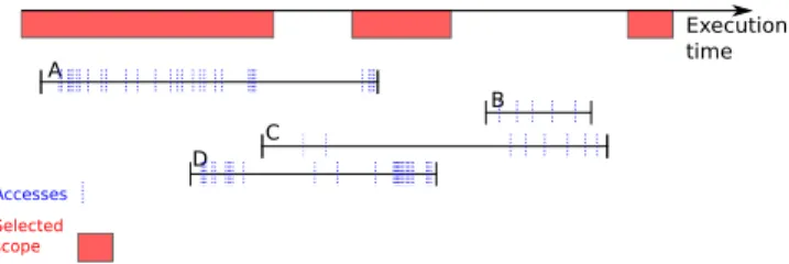
other. The figure 1 represents an exemple of data A, B, C and
2This is similar to a hot spots method profiling one can achieve with gprof
on a sequential program
D which belong to the setsW , U , U and V respectively, and
their accesses. Execution time A B C D Accesses Selected scope
Figure 1. Lifespan and accesses distribution over time
N = W ∪ U ∪ V (13)
Data accessed exclusively inside or outside of selected scopes Data which are only accessed in non selected scopes are not considered as potential candidates to be allocated on studied memory. For each of these data, either the speedup induced would be marginal (cold-spot) or there would be
a slowdown induced because∀j ∈ [[1; M]], t[i j] > t. That
means, for the metrics used, there is no way to speedup the application execution time by storing the data on a memory
different from the main memory. ThusU is excluded from
the set of data to consider when solving DAMMLP, and data in this set will remain allocated on main memory. Besides, the set D defining capacity constraint complexity is also reduced, as these data will never be considered in overlap-ping lifespan groups. On the contrary, data accessed only in selected scopes, in contrast to data accessed in both type of scopes, are marked as important data to the DAMMLP resolution. Their objective coefficient value is updated in consequence.
Data accessed in both selected and non selected scopes For these data accessed in both types of scopes, selection is more complex. A conservative approach is to consider removing them from the search space. Since these data can be used in non selected scopes, these accesses may infer
some slowdown. By removing them, the new set of dataNs
considered when solving the DAMMLP is only composed of
data accessed only in selected scopes. Thus,Ns=W . However
this may remove a lot of data from the search space, including data which may have brought speedup, hence leading to a less optimal solution.
To avoid that, we will consider the new set of data as
composed of all data accessed in selected scopes (Ns=W ∪V ),
and we will try to remove data bringing no speedup. Focusing
on one of these datai, the program execution time can be
divided into three parts. The timexi spent in the union of
selected scopes in which this data is accessed, the timeyi
spent in the union of non selected scopes in which this data
Data Allocation Method MEMSYS’18, October 2018, The Washington DC Area, DC, United States
is accessed, and the timeziof the remaining scopes in which
this data is not accessed. The program execution time can be
expressed as the sum of these three times:ti = xi + yi + zi.
Focusing on one of the HMA memory different from the
main memory,S is the maximum speedup reachable and s is
the minimum slowdown. On the one hand, memory accesses in non selected scopes are slowing down the application by a
factors at worst. On the other hand, the selected scopes are
speeding-up the application by a factorS at best. Allocating
studied data on this memory, program execution time can
be expressed as a function ofxi,yi, zi, s and S (see equation
14).
Ti = xi/S + yi/s + zi (14)
Thus, to keep this data in our search space,Ti must be
less thanti, which leads to a threshold of 1−1/S1/s −1 ×yi forxi,
depending onyi,s and S, as detailed in equation 15.
Ti < ti xi/S + yi/s + zi < xi+ yi+ zi xi/S + yi/s < xi+ yi yi.(1/s − 1) < xi.(1 − 1/S) xi > 1/s − 1 1 − 1/S.yi (15)
If the threshold is respected, memory accesses in non selected scope can be ignored for evaluating data allocation
profit. Thus the datai is considered as being accessed only
in selected scopes and are kept in the search space. On the
contrary, if the threshold is not respected, the datai should
be considered as being accessed only in non selected scopes, and should be removed from the new set.
3.2.2 Comparing data accessed in the same scope
So far, we focused on the data selection out of scope based metrics. However, several data may be accessed in one scope. Each data does not contribute with the same force to mem-ory trafic. To be able to allocate each data differently, data specific weight should be available, and not only scope-wise weight. Data specific weight can be obtain with state-of-the-art methods based on data oriented analysis [23]. Based on state-of-the-art methods which provide weights to data al-location linear problem variables, our method reduces the number of variables while refining the grain of the previous analyses.
4
Design and Implementation
In this section we present the implementation of our scope-based profile-guided method. First, we detail the framework, which is divided into two sections: Scope Selection and Data Extraction. Afterwards, the metric we used to apply our framework to a specific Heterogeneous Memory Architec-ture is described. Finally, we detail the tool we developed to
automatically allocate dynamically allocated data according to ensued allocation strategy during program execution.
4.1 Scope Selection part
Our method is based on a precise, user guided, time profile of the application. Thus, we have implemented a dynamic library managing scope timers, as well as a GCC-6.3.0 plugin to automatically instrument functions and OpenMP parallel regions. A configuration file allows to precisely select which functions to instrument. It is also possible to insert more probes manually if one wants more specific and meaningful scopes.
Finally, the target application time profile is generated by analyzing a trace obtain with our dynamic library. If one does not want an OpenMP pragma granularity, but just function profile, other time profiling tools like Oprofile [16], which is a tool based on hardware counter sampling allowing to have a precise profile of relative time spent inside each program function, may be used.
4.2 Data Extraction part
To extract program data accessed in selected scope, we have implemented a dynamic library wrapping dynamic alloca-tions.
A GCC plugin allows to easily instruments load and store in scopes of interests. This plugin reads a configuration file containing identifiers for scope of interests to focus on. This library implements a function intrument_load_store, which will be called before every load or store one wants to instrument. The library also provides glibc functions malloc, realloc and calloc wrappers. Using LD_PRELOAD mecha-nism, the library wraps dynamic allocations. During the execution, instrumented load and store are registered inside structure linking them to the dynamic allocation they access. This library also implements the algorithm 1 building the set D for respecting memory capacity constraints.
4.3 Metric used
In this section, the metric used for profiling application on a Heterogeneous Memory Architectures – HMA – made of one High Bandwidth Memory – HBM – and one Low Bandwidth Memory – LBM –is detailed. The HBM has less capacity than the LBM which is the system main memory.
Bandwidth Bandit based metric The Bandwidth Ban-dit [4, 8] consists in a banBan-dit application robbing some of the available bandwidth to stress the performance of an application. Our Bandwidth Bandit tool, by sketching the performance derivative with respect to the available memory-bandwidth, makes it possible to qualitatively predict an appli-cation performance variation between HBM and LBM. The Bandwidth Bandit metric is the slowdown factor computed
for each scope between two application runs: one with band-width bandit activated, other without bandband-width bandit. We used this metric for our scope selection.
Load Store count metric As seen in section 3.2.2, some scopes may contain access to distinct dynamically allocated data. In this case, to attribute different profit coefficient to each data, it is necessary to use a metric inside every selected scope. We use the dynamic count of load and store.
4.4 Finding and applying an allocation strategy
The goal of the framework is to profile a scientific application in order to solve the Data Allocation on Multiple Memories Linear Problem. Once the profiling is done using our scope-based method and state of the art metric, the trace text file is read by some python scripts which implements a greedy algorithm for finding a solution. This algorithm sorts data in decreasing profit value order and allocates data on HBM while the memory capacity constraints (cf section 2.3.2) is respected. Once a solution to the DAMMLP has been found, the application can be executed with the allocation strategy implemented. To automatically allocate dynamic data on HBM or LBM according to the strategy, a dynamic allocation wrapper (SwitchTender) has been implemented. The library intercepts allocations and allocates on different memory ac-cording to the inserted probes. The final decision of inserting these probes according the allocation strategy given by our framework or not are left to the end-user.
5
Experimental Environment
In this section we detail the environment used for the method experimental evaluation.
5.1 Hardware setup
The profiling is done on a two sockets Non Uniform Mem-ory Access (NUMA) Architecture. Each node is equipped with a 8 cores Intel Sandy Bridge processor 2,7 GHz, with 32 GB of memory DDR-3 with about 36 GB/s –measured with STREAM, running with 8 threads– and 20MB of LLC. NUMA nodes are linked with Intel Quick Path Interconnect tech-nology, STREAM bandwidth between NUMA nodes yielded about 18 GB/s with 8 threads.
The method evaluation consists in comparing different execution of the same application using different data place-ment or allocation strategies. The material used for the method evaluation is a 68-core KNL processor, of which 4 cores are locked for kernel use. It is configured with 96 GB of DDR4 and 16 GB of MCDRAM. Measuring memory band-width with STREAM benchmark, results show that memory bandwidth usage of a scope-data couple is very complex. Indeed it depends on the static operational intensity, the number of threads, the accesses regularity, threads place-ment on NUMA nodes and hyperthreads processing units, optimization flags (for example on vectorization), etc. On
MCDRAM, it varies from about 10GB/s with any STREAM benchmark running with only one thread and no vectoriza-tion to about 475 GB/s on STREAM benchmark Add compiled with vectorization flag -xMIC-AVX512 with 64 threads scat-tered on all cores. On DDR4 it varies from approximately 10 to about 90 GB/s with same best optimized configura-tion. Note that running only one thread, memory bandwidth usage are equivalent on DDR4 or MCDRAM KNL memories. The measured access latency is 10% longer on MCDRAM than on DDR4. It was measured with a pointer chasing like application extract and tuned from LMBENCH2 benchmarks suite. Thus on the INTEL Knight’s Landing used for our ex-periments the MCDRAM has approximately 6x less capacity, about 5x better bandwidth and approximately 10% worst latency than the DDR4.
5.2 Benchmarks and Mini-applications
In this section we quickly describe the benchmarks used for our method evaluation.
LULESH [11, 12] represents a typical hydrocode. It is a highly simplified application, hard-coded to only solve a simple Sedov blast problem with analytic answers. It repre-sents the numerical algorithms, data motion, and program-ming style typical in scientific C or C++ based applications. LULESH approximates the hydrodynamics equations dis-cretely by partitioning the spatial problem domain into a collection of volumetric elements defined by a mesh. A node on the mesh is a point where mesh lines intersect. LULESH is built on the concept of an unstructured hex mesh. Whereas the default test case for LULESH appears to be a regular Cartesian mesh, the unstructured data structures are repre-sentative of a more complex geometry. We used the OpenMP version 2.0 of the available benchmark.
miniFE is a Finite Element mini application which imple-ments a couple of kernels representative of implicit finite element applications. Running on one node solving a
prob-lem size about 2563is considered as a small problem, contrary
to medium and large problem. This application comes from the Mantevo project [9].
HydroMM is a mini-application which solves a similar problem to that solved by the Hydro2D [27] application. The primary difference between HydroMM and Hydro2D is the presence of multiple materials. HydroMM is highly parallel, based on OpenMP pragma.
5.3 Software setup
During profile phase, each application is compiled with GCC version 6.3.0, optimization flag O3. A part from HydroMM which is compiled with ICC, because it has been optimized for it.
Data Allocation Method MEMSYS’18, October 2018, The Washington DC Area, DC, United States
6
Evaluation
In this section we evaluate our 3 distinct phase approach. First, we profile the application using our scope-based pro-filing tool. This first part allows to reduce the initial data allocation problem complexity, together with attributing val-ues to each dynamic data considered. Second, we solve the data allocation linear reduced problem with an heuristic, implemented in python scripts. Finally, we use our dynamic library wrapper tool to switch the dynamic allocation to the chosen memory at run time.
6.1 Profiling part
We have compared, the sensitivity of tested applications to our bandwidth bandit tool against different input parameters. This confirm the idea that, for tested applications, above a certain threshold, the profiling step of our method does no longer depends on some chosen input parameters such as problem size or number of iterations. Thus a solution obtained with small execution time on small size can easily be extended to bigger problem size of the same application.
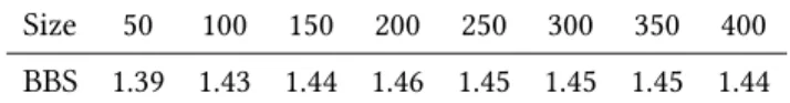
Size BBS 50 1.12 100 1.20 150 1.34 200 1.37 250 1.38 300 1.39
(a) Different sizes. 30 iterations Iterations BBS 1 1.13 10 1.20 20 1.20 30 1.20 40 1.22 50 1.22 (b) Different iterations. Size 100 Iterations BBS 1 1.20 10 1.32 20 1.33 30 1.34 40 1.34 50 1.35 (c) Different iterations. Size 150
Figure 2. LULESH Bandwidth Bandit sensitivity (BBS) against input parameters
Size 50 100 150 200 250 300 350 400
BBS 1.39 1.43 1.44 1.46 1.45 1.45 1.45 1.44
Figure 3. MiniFE Bandwidth Bandit sensitivity (BBS) against input parameters, 200 iterations
The table in figure 2 shows the whole application sensitiv-ity to our Bandwidth Bandit tool (explained in section 4.3), when ran on INTEL sandy nodes. Each Bandwidth Bandit Sensitivity (BBS) represents the slowdown between the
appli-cation run with and without bandit impact3. The bandwidth
sensitivity increases with problem size up to a certain thresh-old depending on the application. These experiments show
3It could be tested by placing data directly on the memory one wants to
test, but the Bandit allows to test memories not available, and problem size with memory usage bigger than MCDRAM capacity
that the problem size must be big enough to profile the ap-plication with our tool, but to run a bigger problem size the application must not be profiled again, the bandwidth sensi-tivity remains correct. In figures 2 and 3, each result is the mean of ten runs and the relative standard deviation for each result is less than 0.5%.
0 50 100 150 200 250
LULESH MINIFE HYDROMM
Number of data objects
Different benchmarks
Total Number of Data Objects Number of Data Objects selected with our method
Figure 4. Number of data objects as Data Allocation Problem variables
Applying our scope-based dataset reduction method (cf section 3.2.1, inequation 15) to the Intel Knight’s Landing
HMA,S = 5 (MCDRAM bandwidth maximum speedup over
DDR4) ands = 0.9 (MCDRAM latency minimum slowdown
over DDR4), thusx > 0.14 × y. In theory, the time spent
inside selected scopes accessing a specific data must be at least 0.14 times greater than the time spent accessing this data inside non selected scopes, if one wants to be sure that the data is a good candidate for MCDRAM. In practice, we have made the assumption that the inequation is always true. This way, we were not obliged to instrument load and store inside non selected scopes and profiling overhead have been kept to an acceptable level (between x5 and x30, comparing with x100 of Valgrind based profiling).
Our method allows to reduce the number of data which must be treated in order to solve the data placement problem. The number of data dynamically allocated may depend on application input parameters. On LULESH for example, at runtime, the number of dynamically allocated data increases with the number of iterations. Nevertheless, our method is applied to the code location of dynamically allocated data. This is named data object (or memory object) in some previous work [10, 19, 24]. More precisely, in our paper a data object is uniquely defined by the call stack obtained when wrapping the malloc (or realloc or calloc) glibc call. This call stack is obtained with a call to the backtrace and backtrace_symbols functions (glibc 2.1). Thus different dynamically allocated arrays may correspond to the same data object. The num-ber of application data objects does not depend on input parameters such as problem size or number of iterations. Consequently, the reduction of the data allocation problem complexity does not depend on application input parameters like problem size or number of iterations.
The graph in figure 4 shows the dynamic data allocation problem complexity reduction obtained with our method. One third for LULESH, two third for HydroMM and 98% for MiniFE. The drastic reduction in MiniFE programs is due to the use of YAML based library which induces great amount of dynamically allocated data. Our method allows to not consider the part of the code accessing to these data, thus drastically reducing the data object to consider in the data allocation problem resolution.
6.2 KNL speedup evaluation
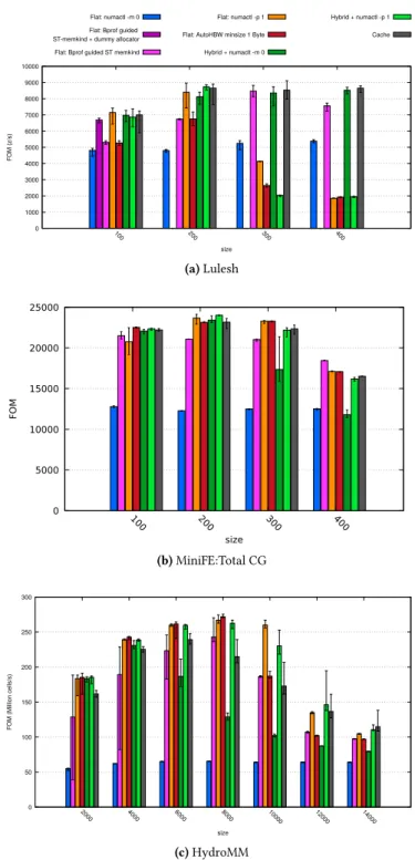
In this section we compare our method to other known pos-sibility to manage MCDRAM on INTEL Knight’s Landing processor. The graphs in figure 7 show the applications mem-ory usage peak against problem size as well as the KNL MC-DRAM memory capacity (16GB). The memory usage peak does not depends on number of iterations count, that is why the graph shows only one value per size. We note that for a problem size between 250 and 300 the memory usage ex-ceed MCDRAM memory capacity for LULESH. For MiniFE it is between 300 and 400. As HydroMM is concerned, the threshold is located between problems of size 6500 and 7000. The graphs contained in figures 5 and 6 shows the differ-ent application Figure Of Merit (FOM) against problem sizes. The programs are executed on a single INTEL KNL node of 64 cores, each core contains 4 Processing Unit (hyper-threads technology). We ran LULESH and MiniFE OpenMP version with 64 threads each, one per core. We ran HydroMM with 128 threads because this number of threads, two hyper-threads per core, maximizes the application performance.
For each graph the different configurations, in the legend, are:
• numactl -m 0: KNL with MCDRAM in flat mode, using numactl command to put all data on DDR4.
• Flat: Bprof guided ST memkind: using our profiling tool Bprof (Bandwidth Bandit Profiler) to select the data. Then, during program execution the dynamically allocated data are allocated by our dynamic library wrapper: SwitchTender.
• Flat: Bprof guided ST memkind + dummy allocator: same as precedent plus a dummy allocator. This locator is just here to avoid doing many dynamic al-locations when allocating data on MCDRAM through a call to hbw_malloc/realloc/calloc. It shows that for small problem size on LULESH, the memkind library adds a non marginal overhead.
• numactl -p 1: KNL with MCDRAM in flat mode, using numactl command to try to put data on MCDRAM, the strategy is first-come first-served.
• AutoHBW: using dynamic library AutoHBW, built upon memkind library [3, 6]. AutoHBW uses the same strategy as numactl -p 1 but it let the possibility to
0 1000 2000 3000 4000 5000 6000 7000 8000 9000 10000 100 200 300 400 FOM (z /s) size Flat: numactl -m 0
Flat: Bprof guided ST-memkind + dummy allocator Flat: Bprof guided ST memkind
Flat: numactl -p 1 Flat: AutoHBW minsize 1 Byte Hybrid + numaclt -m 0 Hybrid + numactl -p 1 Cache (a) Lulesh 0 5000 10000 15000 20000 25000 100 200 300 400 FOM size (b) MiniFE:Total CG 0 50 100 150 200 250 300 2000 4000 6000 8000 10000 12000 14000 FOM (M illion ce lls/s) size (c) HydroMM Figure 5. KNL performances
precise a minimum data size threshold from which to allocate data on MCDRAM.
• Hybrid + numactl -m 0: KNL with MCDRAM in hybrid mode, half as a cache, and half in flat mode. Besides the command numactl -m 0, data are store on DDR4, none of the flat capacity of the MCDRAM is used. Then
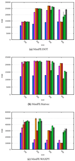
Data Allocation Method MEMSYS’18, October 2018, The Washington DC Area, DC, United States 0 5000 10000 15000 20000 25000 30000 100 200 300 400 FOM size (a) MiniFE:DOT 0 5000 10000 15000 20000 25000 100 200 300 400 FOM size (b) MiniFE:Matvec 0 10000 20000 30000 40000 50000 60000 100 200 300 400 FOM size (c) MiniFE:WAXPY
Figure 6. MiniFE performance details on KNL
this is as if the MCDRAM cache was half of its usual capacity.
• Hybrid + numactl -p 1: KNL with MCDRAM in hybrid mode, half as a cache, and half in flat mode. Besides the command numactl -p 1 is used.
• Cache: KNL with MCDRAM in cache mode.
For each graph, the result is the mean of 10 runs with error bars. The graph 5a shows the Figure Of Merit (FOM) obtained
executing LULESH. On small size (100= 1GB < 16GB), our
method allows to select only the right data object to store on MCDRAM in order to have the same speedup as if all
0 10 20 30 40 50 60 70 100 150 200 250 300 350 400 V irtual Memory P eak (GB)
Different problem sizes Memory Usage
MCDRAM memory capacity
(a) Lulesh 0 5 10 15 20 25 100 200 300 400 V irtual Memory P eak (GB)
Different problem sizes (nx=ny=nz) Memory Usage
MCDRAM memory capacity
(b) MiniFE 0 5 10 15 20 25 30 35 40 2000 3000 4000 5000 6000 6500 7000 8000 9000 10000 11000 12000 V irtual Memory P eak (GB)
Different problem sizes Memory Usage
MCDRAM memory capacity
(c) HydroMM
Figure 7. Application memory usage
data were store on MCDRAM (numactl -p 1). This is only true using our dummy allocator to avoid the overhead due to multiple call to memkind allocator. For a size of 200, the result with dummy allocator is not possible because there are too much allocations for it to handle. For sizes bigger than MCDRAM capacity (300 and 400) our method allows to select the right data to keep on MCDRAM and it is as good as MCDRAM in cache mode.
The graph 5b shows the FOM obtained executing MiniFE. MiniFE is composed of a dot, a matvec and a waxpy opera-tions. Thus the graphs in figure 6 detail the result of MiniFE Total CG (Conjugate Gradient). These graphs show that, considering the total execution time, our method stick with the best method’s result. Looking at the decomposition of MiniFE results, we see that our method does not allocated data object used in WAXPY operation on MCDRAM. This is because these data are automatically and statically allocated
on the stack. Thus our dynamic library wrapping dynami-cally allocated data can not consider them as potential data objects to be stored on MCDRAM. This is a limitation which could be overcome with a binary instrumentation as it is possible to do with PIN. Nevertheless, the other data ob-jects responsible for the memory bandwidth sensitivity of MiniFE kernels are dynamically allocated. Then, despite this limitation, our method successfully highlights data objects which, once allocated on MCDRAM, bring speedup to the application execution time.
The graph 5c shows the FOM obtained executing Hy-droMM. For problem size between 2000 and 6000 (memory usage peak is below the MCDRAM memory capacity), our method gives erratic results. Our dynamic allocation library contains threads locks, then the time to make allocation decisions may be erratic because of the non synchronized threads behavior. Thus, the error bars may be linked to the ratio of number of allocations per seconds. Indeed, the total execution time for these problem sizes is short (less than one second), thus it is more sensitive to the time spent in our library decision making execution. For other problem size we have similar results compare to other methods. The performance drop visible from size 10000 is due to the fact that the memory usage of the data objects considered as sensitive to memory bandwidth exceed MCDRAM capacity. Indeed, in HydroMM there are not so much data objects, but they contain all data, so their memory usage is big. As it is not possible for our tool to cut data objects in pieces to just place some bandwidth sensitive data on MCDRAM, the High Bandwidth Memory is underutilized. Whereas with the MC-DRAM in Cache mode or with MCMC-DRAM in flat mode but using numactl -p 1 command, the system manipulates 4kB page size (even less for cache). Then these methods continue to have speedup, they have not our underutilization limit problem. Finally, with a finer grain, our method could con-tinue to allocate data on the high bandwidth memory, that is why some future works go in the direction of an allocator able to use our method insights.
7
Related Work
In the introduction some objectives have been highlighted as key steps to follow in the data allocation problem resolution. For reminder there are four: (I ) Formulation, (II ) objective function coefficients evaluation, (III ) solver (heuristic) design and (IV ) data allocation technical solution. All these four points have been partially tackled by some previous work. Formulation (I) In [13], the authors developped a frame-work for generating High Performance Fortran-style data layout specifications in a way which is close to our approach. But, to the best of our knowledge, a clear formulation of the Data Allocation on HMA problem has never been written. In [26] there is a reference to the knapsack problem. Ac-cording to the authors, because of potentially hundreds of
memory objects and large memory levels, computing a pure 0/1 knapsack problem has proved to be impractical in their experiments. Nevertheless, as shown at the end of section 6.1, the number of variables is not excessive if the data objects, opposed to every single dynamically allocated data, are con-sidered as variables. Moreover, our method shows that even in code with hundreds of data objects such as MiniFE it may be possible to reduce drastically this number with a temporal then spatial analysis (cf section 6.1).
Objective function coefficients evaluation (II) Some
works have proposed metrics to evaluate data regarding the different memories on which it could be allocated. Whereas Profile-Guided evaluation based on LLCmiss hardware coun-ters [26] are architecture dependent, our metric based on a bandwidth bandit [4, 8] allows to sketch the application sensitivity to any memory bandwidth. Morever, LLCmiss count may not be precise enough to evaluate bandwidth sen-sitivity, and hardware counters must be carefully measured to extract relevent information [10].
Instead of attributing weight to the data objects, Ivy Bo Peng et al. [25] enunciate some rules, based on mini-benchmark evaluations, to choose on which memory one data should be allocated. Since they build their heuristic without trying to weight the different data objects, they limit the problem resolution to their unique heuristic.
Some static metrics have been tested [14], but they are difficult to manage on mini-application bigger than small benchmarks, and the information extracted are not relevant enough. Besides, pointer aliasing makes it very difficult, if not impossible, to have good information on all data objects. Finally, static load and store count gives not enough informa-tion about how much the memory performances are stressed. This is due to CPU caching and it is possible to analyse this effect statically [1, 5], or dynamically [31].
Problem solving and heuristics (III) From Benchmarks evaluation Ivy Bo Peng et al. have developed a heuristic tuned to the INTEL Knight’s Landing processor Heteroge-neous Memory Architecture to attribute to each dynamically or statically allocated data object a memory between MC-DRAM flat, MCMC-DRAM cache and DDR4. The choice is based on several metrics: number of threads accessing the data, data memory usage, operational intensity and access pattern. Then, their heuristic follows these rules to allocate data ob-jects on the appropriate memory. These rules allow them to make the difference between latency and bandwidth sen-sitive data object, thus they manage to exceed MCDRAM as a cache performance on memory latency sensitive codes (Graph500, XSBench). Our scope-based method could en-hance this analysis by highlighting the scope to analyze, therefore maybe reducing the analysis overhead.
In [26] the authors use a greedy algorithm: data object are sorted against LLC miss count, or LLC miss count divided by the data object size. Then they allocate on MCDRAM the
Data Allocation Method MEMSYS’18, October 2018, The Washington DC Area, DC, United States element of the sorted list until the memory capacity limit
is reached. Nevertheless, their method does not take over-lapping data lifespan, thus they must give their framework a false High Bandwidth Memory size in order for it to put enough data to have good performance. It is not the case with our framework, as it is based on a more accurate data allocation problem formulation which takes data lifespan into account in the constraints.
In [17], the authors study the impact of two different on-package memories on some HPC kernels performance (Dense and sparse matrices operations, cholesky, FFT, stencil and STREAM). The two memories are the KNL MCDRAM (cache, hybrid and flat mode) and the broadwell eDRAM (only cache mode). They develop a new model, the stepping model, which allow them to give some advice on how to place data on heterogeneous memory architecture. Never-theless, they do not differentiate the different dynamically allocated data inside an application.
In [7], the authors have made a PIN based profiling tool which captures load and store accesses. They also have imple-mented two heuristics to solve the data allocation problem. Our method permit to leverage their approach in reducing the amount of data which are necessary to be studied to solve the data allocation problem.
Data allocation technical solution (IV) In [26] the au-thors present an automatic allocation based on dynamic allo-cation wrapper library. Nevertheless, there is a non marginal overhead due to glibc backtrace function call on each dy-namic data allocation wrapped. Indeed, to know if a dynami-cally allocated data must be allocated on the KNL MCDRAM, they compare the data object call stack with each call stack contained in a text file filled during application profiling. On the contrary, our framework is based on code instrumenta-tion with probes wrapping the funcinstrumenta-tion call which includes the less other data objects (cf data object definition in sec-tion 6.1). Finally, our method is more user demanding in pre-program execution stage, because the user (or compiler pass) must instrument the code, but there is no overhead during the program execution.
In [14] the authors suggest a LLVM pass to change calls to malloc into calls to hbw_malloc, from the memkind dynamic library. The approach is too limited to work on C++ mini-application because of the presence of objects wrapping malloc calls.
8
Conclusion
In this paper we have formulated the Data Allocation Prob-lem towards the goal of minimizing the application execu-tion time. From this formulaexecu-tion we have deduced, under the assumption that each data allocation does not influence memory performance, a linear formulation: the Data Alloca-tion Linear Problem. Then this problem can be solved as a
linear optimization problem. The difficulty lies in the com-putation of the objective coefficients, and the great number of variables (program dynamically allocated data). Thus, we have develop a Profile-Guided Scope-Based method to re-duce the problem complexity, removing data which are only used in execution time cold-spot, as data which are not used in memory sensitive hot-spot.
Focusing on a Heterogeneous Memory Architecture made of one High Bandwidth Memory/Low Bandwidth Memory (HBM/LBM-HMA), we use a bandwidth sensitive metric and our method to approximate the Data Allocation Linear Prob-lem objective coefficients. We validate our results using Intel Knight’s Landing many-core processor as a HBM/LBM-HMA real architecture. Whereas our Scope Based Profiling method shows great results, the Load Store count metric (cf sec-tion 4.3) used to distinct data inside each scope should be enhanced with program locality analysis in future work, therefore completing our scope selection based on Band-width Bandit.
In our problem formulation we have chosen to minimize the execution time as objective of our optimization prob-lem, but the formulation could be easily adapted to other objective. For example, the objective function could focus on energy consumption. The difficulty would then be to have an efficient metric to predict the energy consumption coefficient of the objective function. Finally, the problem for-mulation could take critical memory usage into its objective function. This would lead to find an optimal solution to the data allocation problem relative to the problem of storing the most critical data on Non Volatile Memory for a program using checkpoint/restart paradigm. Here again, the difficulty would be to have the right objective coefficient for the data: how much a data is critical to the program ?
A
Headings in Appendices
References
[1] Wenlei Bao, Sriram Krishnamoorthy, Louis-Noel Pouchet, and P. Sa-dayappan. 2017. Analytical Modeling of Cache Behavior for Affine Programs. Proc. ACM Program. Lang. 2, POPL, Article 32 (Dec. 2017), 26 pages. https://doi.org/10.1145/3158120
[2] E. Bolotin, D. Nellans, O. Villa, M. O’Connor, A. Ramirez, and S.W. Keckler. 2015. Designing Efficient Heterogeneous Memory Architec-tures. Micro, IEEE 35, 4 (July 2015), 60–68. https://doi.org/10.1109/ MM.2015.72
[3] Christopher Cantalupo, Vishwanath Venkatesan, Jeff Hammond, Krzysztof Czurlyo, and Simon David Hammond. 2015. memkind: An Extensible Heap Memory Manager for Heterogeneous Memory Platforms and Mixed Memory Policies. (3 2015).
[4] Marc Casas and Greg Bronevetsky. 2014. Active Measurement of Mem-ory Resource Consumption. In 2014 IEEE 28th International Parallel and Distributed Processing Symposium, Phoenix, AZ, USA, May 19-23, 2014. IEEE Computer Society, 995–1004. https://doi.org/10.1109/IPDPS. 2014.105
[5] Dong Chen, Fangzhou Liu, Chen Ding, and Sreepathi Pai. 2018. Local-ity Analysis through Static Parallel Sampling. In Proceedings of the 39th 13
ACM SIGPLAN Conference on Programming Language Design and Im-plementation, PLDI 2018, Philadelphia, Pennsylvania, the United States, June 18-22, 2018.
[6] Intel Corporation. [n. d.]. hbwmalloc man page. https://www.mankier. com/3/hbwmalloc. ([n. d.]). [Online; accessed 26-june-2017]. [7] T. Effler, Adam Howard, Tong Zhou, Michael R. Jantz, Kshitij A. Doshi,
and Prasad A. Kulkarni. 2018. On Automated Feedback-Driven Data Placement in Multi-tiered Memory.
[8] David Eklov, Nikos Nikoleris, David Black-Schaffer, and Erik Hager-sten. 2013. Bandwidth Bandit: Quantitative characterization of mem-ory contention. In CGO. IEEE Computer Society, 10. https://doi.org/ 10.1109/CGO.2013.6494987
[9] Michael A Heroux, Douglas W Doerfler, Paul S Crozier, James M Willenbring, H Carter Edwards, Alan Williams, Mahesh Rajan, Eric R Keiter, Heidi K Thornquist, and Robert W Numrich. 2009. Improving Performance via Mini-applications. Technical Report SAND2009-5574. Sandia National Laboratories.
[10] Marty Itzkowitz, Brian J. N. Wylie, Christopher Aoki, and Nicolai Kosche. 2003. Memory Profiling Using Hardware Counters. In Proceed-ings of the 2003 ACM/IEEE Conference on Supercomputing (SC ’03). ACM, New York, NY, USA, 17–. https://doi.org/10.1145/1048935.1050168 [11] Ian Karlin, Abhinav. Bhatele, Bradford L.. Chamberlain, Jonathan.
Co-hen, Zachary Devito, Maya Gokhale, Riyaz Haque, Rich Hornung, Jeff Keasler, Dan Laney, Edward Luke, Scott Lloyd, Jim McGraw, Rob Neely, David Richards, Martin Schulz, Charle H. Still, Felix Wang, and Daniel Wong. 2012. LULESH Programming Model and Performance Ports Overview. Technical Report LLNL-TR-608824. 1–17 pages. [12] Ian Karlin, Jeff Keasler, and Rob Neely. 2013. LULESH 2.0 Updates and
Changes. Technical Report LLNL-TR-641973. 1–9 pages.
[13] Ken Kennedy and Ulrich Kremer. 1998. Automatic Data Layout for Distributed-memory Machines. ACM Trans. Program. Lang. Syst. 20, 4 (July 1998), 869–916. https://doi.org/10.1145/291891.291901 [14] Dounia Khaldi and Barbara M. Chapman. 2016. Towards Automatic
HBM Allocation Using LLVM: A Case Study with Knights Landing. In Third Workshop on the LLVM Compiler Infrastructure in HPC, LLVM-HPC@SC 2016, Salt Lake City, UT, USA, November 14, 2016.
[15] Min Lee, Vishal Gupta, and Karsten Schwan. 2013. Software-controlled Transparent Management of Heterogeneous Memory Resources in Virtualized Systems. In Proceedings of the ACM SIGPLAN Workshop on Memory Systems Performance and Correctness (MSPC ’13). ACM, New York, NY, USA, Article 5, 6 pages. https://doi.org/10.1145/2492408. 2492416
[16] John Levon and Philippe Elie. 2004. Oprofile: A system profiler for linux. (2004).
[17] Ang Li, Weifeng Liu, Mads R. B. Kristensen, Brian Vinter, Hao Wang, Kaixi Hou, Andres Marquez, and Shuaiwen Leon Song. 2017. Exploring and Analyzing the Real Impact of Modern On-package Memory on HPC Scientific Kernels. In Proceedings of the International Conference for High Performance Computing, Networking, Storage and Analysis (SC ’17). ACM, New York, NY, USA, Article 26, 14 pages. https://doi.org/ 10.1145/3126908.3126931
[18] Felix Xiaozhu Lin and Xu Liu. 2016. Memif: Towards Programming Heterogeneous Memory Asynchronously. In Proceedings of the Twenty-First International Conference on Architectural Support for Programming Languages and Operating Systems (ASPLOS ’16). ACM, New York, NY, USA, 369–383. https://doi.org/10.1145/2872362.2872401
[19] Margaret Martonosi, Anoop Gupta, and Thomas Anderson. 1992. Mem-Spy: Analyzing Memory System Bottlenecks in Programs. SIGMETRICS Perform. Eval. Rev. 20, 1 (June 1992), 1–12. https://doi.org/10.1145/ 149439.133079
[20] M.R. Meswani, S. Blagodurov, D. Roberts, J. Slice, M. Ignatowski, and G.H. Loh. 2015. Heterogeneous memory architectures: A HW/SW approach for mixing die-stacked and off-package memories. In High Performance Computer Architecture (HPCA), 2015 IEEE 21st International
Symposium on. 126–136. https://doi.org/10.1109/HPCA.2015.7056027 [21] Mitesh R. Meswani, Gabriel H. Loh, Sergey Blagodurov, David Roberts, John Slice, and Mike Ignatowski. 2014. Toward Efficient Programmer-managed Two-level Memory Hierarchies in Exascale Computers. In Proceedings of the 1st International Workshop on Hardware-Software Co-Design for High Performance Computing (Co-HPC ’14). IEEE Press, Piscataway, NJ, USA, 9–16. https://doi.org/10.1109/Co-HPC.2014.8 [22] Sparsh Mittal and Jeffrey S. Vetter. 2016. A Survey Of Techniques for
Architecting DRAM Caches. IEEE Trans. Parallel Distrib. Syst. 27, 6 (2016), 1852–1863. https://doi.org/10.1109/TPDS.2015.2461155 [23] Antonio Peña and Pavan Balaji. 2016. A data-oriented profiler to assist
in data partitioning and distribution for heterogeneous memory in HPC. 51 (01 2016).
[24] A. J. Peña and P. Balaji. 2014. A Framework for Tracking Memory Ac-cesses in Scientific Applications. In 2014 43rd International Conference on Parallel Processing Workshops. 235–244. https://doi.org/10.1109/ ICPPW.2014.40
[25] Ivy Bo Peng, Roberto Gioiosa, Gokcen Kestor, Pietro Cicotti, Erwin Laure, and Stefano Markidis. 2017. RTHMS: A Tool for Data Placement on Hybrid Memory System. In Proceedings of the 2017 ACM SIGPLAN International Symposium on Memory Management (ISMM 2017). ACM, New York, NY, USA, 82–91. https://doi.org/10.1145/3092255.3092273 [26] H. Servat, A. J. Peña, G. Llort, E. Mercadal, H. C. Hoppe, and J. Labarta. 2017. Automating the Application Data Placement in Hybrid Memory Systems. In 2017 IEEE International Conference on Cluster Computing (CLUSTER). 126–136. https://doi.org/10.1109/CLUSTER.2017.50 [27] Jason Sewall and Guillaume Colin de Verdière. 2015. From “Correct” to
“Correct & Efficient”. 7–42 pages.
[28] A. Sodani, R. Gramunt, J. Corbal, H. S. Kim, K. Vinod, S. Chinthamani, S. Hutsell, R. Agarwal, and Y. C. Liu. 2016. Knights Landing: Second-Generation Intel Xeon Phi Product. IEEE Micro 36, 2 (Mar 2016), 34–46. https://doi.org/10.1109/MM.2016.25
[29] Wm. A. Wulf and Sally A. McKee. 1995. Hitting the Memory Wall: Implications of the Obvious. SIGARCH Comput. Archit. News 23, 1 (March 1995), 20–24. https://doi.org/10.1145/216585.216588 [30] W. Zhang and T. Li. 2009. Exploring Phase Change Memory and 3D
Die-Stacking for Power/Thermal Friendly, Fast and Durable Memory Architectures. In Parallel Architectures and Compilation Techniques, 2009. PACT ’09. 18th International Conference on. 101–112. https: //doi.org/10.1109/PACT.2009.30
[31] Y. Zhong, S. G. Dropsho, X. Shen, A. Studer, and C. Ding. 2007. Miss Rate Prediction Across Program Inputs and Cache Configurations. IEEE Trans. Comput. 56, 3 (March 2007), 328–343. https://doi.org/10. 1109/TC.2007.50