Abstract.
Water managers are concerned about the poor structural state of their water
pipe networks and are confronted with the lack of tools to analyze their data in order to
evaluate both the present and future state of their networks. Researchers have developed
statistical models with the annual number of pipe breaks as an indicator of the structural
state of their networks. Unfortunately, most statistical modeling strategies do not perform
well when used in municipalities with short recorded pipe break histories. Pipe breaks
must have been recorded since the installation of the first pipes, and this is rarely the case
in most municipalities. This paper presents a methodology to estimate calibration
parameters of statistical models in municipalities with short recorded pipe break histories.
The application of this methodology to a municipality with a century-old water pipe
network and a recorded pipe break history of 21 years is also presented.
1. Introduction
The last decades have seen an important number of studies related to the structural state and aging of urban infrastruc-tures in North America. Roads, sidewalks, sewers, water facil-ities, bridges, and other infrastructures are reported to be in poor condition and deteriorating rapidly. In 1985 the Federa-tion of Canadian Municipalities (FCM) published a report on the state of municipal infrastructures based on a survey in many Canadian municipalities. The cost of updating these in-frastructures was estimated to be around 18 billion dollars [Desbiens, 1997]. In 1995 a new survey undertaken by McGill University in conjunction with FCM concluded that the cost had risen to 44 billion dollars for all of Canada [Siddiqui and Mirza, 1996].
“Out of sight, out of mind” aggravates the problem for underground water infrastructure. In the United States, two milestones were at the origin of the realization that major problems existed with older water distribution networks. The first was the passage of the Safe Drinking Water Act of 1974, which mandated that the U.S. Environmental Protection Agency be concerned with the supply of drinking water to consumers. The second was the publication of the report by Choate and Walter [1981], which attempted to draw attention to the “infrastructure crisis.” With pipe breaks and sewer over-flows occurring more frequently, water managers are asking questions about the state of their water and sewer networks, concerned that these infrastructure systems did not receive adequate preventive maintenance.
Although it is quite clear that major interventions are needed on most networks, budget constraints make it essential to better plan and optimize these interventions. The manage-ment of water networks, in terms of optimizing the cost of intervention by better planning repair, rehabilitation, and
re-placement of pipes, has become very complex, and researchers have developed methodologies to help water managers in that task [e.g., Goulter et al., 1993; Kleiner et al., 1998a, 1998b; Villeneuve et al., 1998]. Before cost optimization can be achieved, one must first develop modeling strategies to evalu-ate the present stevalu-ate and predict the evolution of the structural state of networks using available (or easily obtainable) data. The performance of a modeling strategy will depend on the identification of good indicators of the structural state. The resulting pipe break model can serve both as a diagnostic tool (e.g., identification of pipes with high breakage rates) and an optimization tool (e.g., best replacement strategies), but also, when coupled with an economic assessment model, it becomes a powerful tool for decision making for water managers [O’Day et al., 1986].
Survival analysis is a statistical method used for analysis of time-to-failure data. The main advantage of survival analysis is that it takes into account information from pipes that have failed one or more times during the observation period as well as pipes that have not failed during the same period. The main disadvantage is that this type of analysis requires detailed in-formation on the characteristics of pipe segments in the net-work and a long history of pipe breaks. Time to failure between successive breaks was observed to be very different than time to failure from pipe installation to first break [e.g., Clark et al., 1982, 1988; Andreou et al., 1987]. The survival time between different break orders needs to be described by different sta-tistical distributions since they exhibit different breakage be-haviors. The most commonly used statistical distributions for time-to-failure data associated with pipe breaks are the expo-nential and the Weibull distributions [e.g., Andreou et al., 1987; Eisenbeis, 1994]. In order to use survival analysis, time to fail-ure must be known for the entire sequence of pipe breaks, that is, from pipe installation to first break, from first break to second, etc. This is rarely the case, especially for municipalities with older water pipe networks, since their recorded pipe break histories rarely cover the entire history of their network. Copyright 2000 by the American Geophysical Union.
Paper number 2000WR900185. 0043-1397/00/2000WR900185$09.00
Therefore time to failure is only known for breaks that happen within an observation period that usually only covers recent years. Knowledge of the order of breaks (first, second, third, etc.) is only available if the pipe was installed during the time covered by the observation period. This considerably limits the applicability of standard survival analysis in modeling the struc-tural state of water pipe networks.
Many researchers have used survival analysis successfully to evaluate past and present breakage rates and to predict break-age trends in the near future. For example, Karaa and Marks [1990] used Cox’s proportional hazard model to analyze the city of New Haven’s data divided into six installation periods. In Canada, pioneer work has been done by I. C. Goulter’s team on the city of Winnipeg’s water pipe network’s data. Kettler and Goulter [1985] analyzed the breakage rates of grey cast iron and asbestos-cement pipes in relation to pipe diameter and pipe age. Goulter and Kazemi [1988] observed that 22% of pipe breaks occurred within 1 m from one another, and 46% oc-curred within 20 m. Goulter et al. [1993] developed a method-ology to quantify the temporal and spatial groupings of these pipe breaks. Jacobs and Karney [1994] developed two indica-tors of the reliability of a water pipe network: first, the prob-ability of having a day without a pipe break and, second, the probability of having an independent break (not in the vicinity of a recent break). In Germany, Herz [1996] developed his own statistical distribution and used a cohort survival model to estimate breakage and renewal rates on 10 European net-works. In France, Eisenbeis [1994] used Cox’s proportional hazard model to analyze breakages rates on two urban net-works with recorded pipe break histories of 40 and 54 years.
To our knowledge the only two studies that dealt with brief recorded pipe break histories are the ones by Kleiner and Rajani [1999] and Eisenbeis [1994]. These researchers obtained parameter values for different categories of pipes from a gen-eral model developed with recorded pipe break histories cov-ering many decades. The general model used by Kleiner and Rajani [1999] is based on an exponential relationship devel-oped by Shamir and Howard [1979], while, as mentioned above, Eisenbeis [1994] used Cox’s proportional hazard model.
In this paper, we present a methodology which extends the applicability of survival analysis to networks with brief re-corded pipe break histories. The proposed methodology is
different from that of Eisenbeis [1994] and Kleiner and Rajani [1999], since it is formally exact and it explicitly takes into account the fact that we do not know how many and when pipe breaks occurred during the nonrecorded period. It is then possible to include the “older” part of the network in the analysis and to compare the evolution of its structural state with the “younger” part. Comparison of different pipe break models is also possible.
First, we present basic concepts and some terminology, and then we elaborate on mathematical developments and calcu-lations of the likelihood function. Application of this method-ology to the municipality of Chicoutimi (Province of Quebec, Canada) is then presented, and we finally show how two pipe break models can be compared in order to estimate which one is the most significant statistically.
2. Modeling Water Pipe Network Structural
State: Basic Elements
2.1. Discretization of the Network Into Pipe Segments
The water pipe network must be discretized into pipe seg-ments. A pipe segment is a series of pipes with relatively homogeneous characteristics, in terms of what affects the rate of pipe degradation, that usually runs from one street corner to the next (see Figure 1). Previous studies have highlighted the fact that pipe characteristics, such as pipe diameter and type of material, have an impact on the breakage rate [Clark et al., 1982; Andreou et al., 1987]. For example, Kettler and Goulter [1985] have observed that pipe failure rates are much higher for smaller diameters, probably because of the thinner pipe walls. A pipe segment is also the smallest element where a pipe break can be located.
2.2. Modeling Strategy
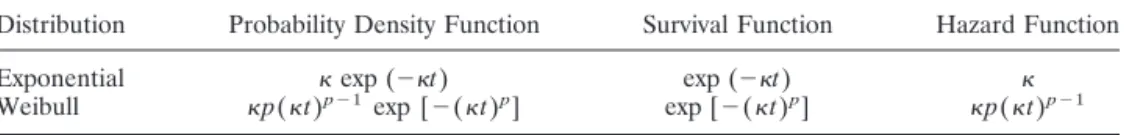
Once the pipe network has been discretized into pipe seg-ments, one must specify the type of probability distribution that will be used to describe each break order. In the present study, two types of probability distribution were considered for modeling time between breaks: a two-parameter Weibull dis-tribution and a one-parameter exponential disdis-tribution (Table 1). These two distributions were applied to different orders of breaks in various combinations as depicted in Table 2. The
age probability with time for each pipe segment. Equations for the survival function F(t), the hazard function(t), and prob-ability density function f(t) for these two distributions are presented in Table 1 (for a definition of these functions see Kalbfleisch and Prentice [1980] or Cox and Oakes [1994]). It is important to note that the developed methodology is applica-ble no matter the types of distributions considered to describe the different break orders. Table 2 presents the different pipe break models considered for our case study. The number of calibration parameters depends on the distributions used and on the number of break orders considered.
Survival analysis is then used to build the likelihood function and to estimate model parameters. The main advantage of survival analysis in modeling pipe breaks is that it takes into account the occurrence of one or many breaks, and the ab-sence of breaks on pipe segments, when estimating the param-eters of the distributions. When a pipe segment has yet to fail at the time of analysis, its time to failure is said to be right-censored [Miller, 1981]. The likelihood function at the time of analysis t is built considering both the break probability for pipe segments that have failed and the survival probability for pipe segments that have not [Miller, 1981; Kalbfleisch and Pren-tice, 1980].
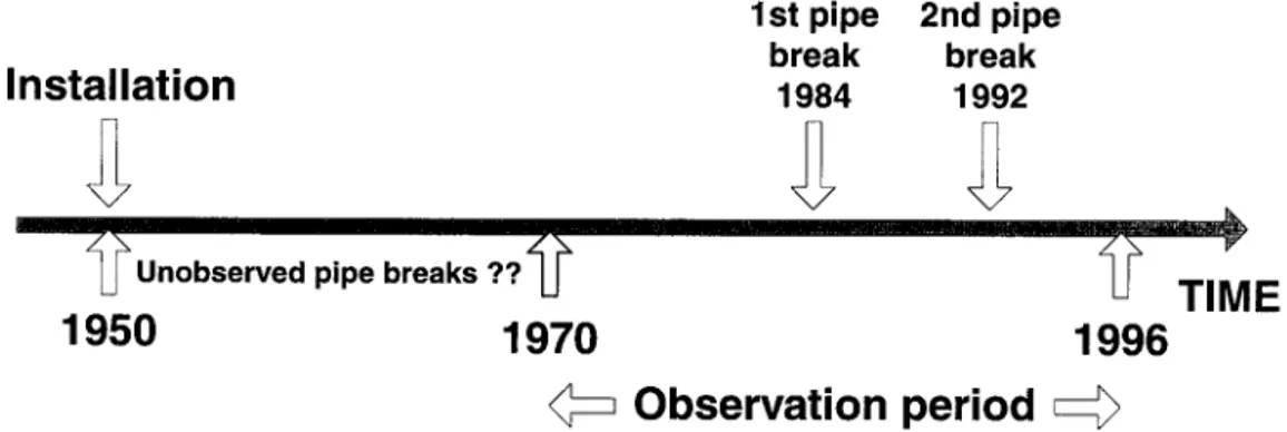
2.3. Specific Problems Associated With Brief Recorded Pipe Break Histories
In order to apply standard survival analysis, it is necessary to have the entire break record since the installation of the first pipes. This is not the case for municipalities with brief re-corded pipe break histories. Figure 2 illustrates this problem for a pipe segment laid in 1950. If pipe breaks have been recorded at least since 1950, then we know that the pipe break in 1985 is the first break and the one in 1990 is the second. However, if pipe breaks began to be recorded in 1976, it is not possible to know if the pipe break observed in 1985 is actually
be noted that unknown information “left” of 1976 cannot be associated to the so-called “left censoring” [Miller, 1981]. Left censoring could only be used if the number of breaks that occurred before 1976 was known, without knowing when these breaks did occur. Knowing the exact order of breaks is key to successfully using survival analysis for modeling pipe breaks, and since this information is not available in municipalities with brief recorded pipe break histories, a new methodology was developed to use at best the information at hand during the observation period.
3. Description of the Proposed Methodology
Our goal is to develop a likelihood function that, once max-imized, will give us the values of the calibration parameters of the distributions associated with the different break orders. The time step used is 1 year. Figure 3 illustrates the case of a pipe segment i that failed  times during the observation period, at times t1, t2, 䡠 䡠 䡠 , and t, and failed␣ times duringthe nonrecorded history, at times t⬘1, t⬘2, 䡠 䡠 䡠 , and t⬘␣. Time t⫽
0 is the time of installation of pipe segment i, Tb is the time when recording began, and Ta is the time of analysis (present time). The nth break order (there are  ⫹ ␣ break orders during a pipe segment’s life) is associated with a statistical distribution and its corresponding probability density function fn(t), survival function Fn(t), and hazard functionn(t).
Probability P(␣, ; {tj}) for a pipe segment i is defined as the probability of occurrence of breaks at times t1, t2, 䡠 䡠 䡠 ,
and tduring the observation period, considering that the pipe
segment already failed␣ times during the nonrecorded history at unknown times t⬘1, t⬘2, 䡠 䡠 䡠 , and t⬘␣. In terms of the different
statistical functions describing the break orders, this probabil-ity is defined by
Table 2. List and Characteristics of Models Considered for the Municipality of Chicoutimi
Models Break Order Distribution Number ofParameters
Weibull-Exponential first break Weibull (1, p1) 3
(W-E) second break and up exponential (2)
Weibull-Exponential-Exponential first break Weibull (1, p1) 4
(W-E-E) second break exponential (2)
third break and up exponential (3)
Weibull-Weibull-Exponential first break Weibull (1, p1) 5
(W-W-E) second break Weibull (2, p2)
third break and up exponential (3)
Weibull-Weibull-Exponential first break Weibull (1, p1) 6 Exponential (W-W-E-E) second break Weibull (2, p2)
third break exponential (3) fourth break and up exponential (4)
P共␣, ; 兵tj其兲 ⫽
冕
0 Tb dt⬘1f1共t⬘1兲冕
t1⬘ Tb dt⬘2f2共t⬘2⫺ t⬘1兲 . . . 䡠冕
t␣⫺1⬘ Tb dt⬘␣f␣共t⬘␣⫺ t⬘␣⫺1兲 f␣⫹1共t1⫺ t⬘␣兲 . . . 䡠 f␣⫹共t⫺ t⫺1兲F␣⫹⫹1共Ta⫺ t兲 dt1. . . dt. (1)Breaks that occur during the nonrecorded history do so in a sequence of arbitrary times {t⬘1, t⬘2, 䡠 䡠 䡠 , t⬘␣}. Since these
times are unknown, the probability of occurrence of the first nonrecorded break is equal to the integral of the probability density function associated with this break order, between the time of installation of the pipe segment (t ⫽ 0) and the time Tbwhen recording began. Each following integral in the equa-tion represents the probability of failure for each higher break order during the nonrecorded history. Obviously, the sequence of breaks must respect the constraint 0ⱕ t⬘1ⱕ t⬘2ⱕ t⬘3䡠 䡠 䡠 ⱕ t⬘␣.
The probability of occurrence of the first recorded break is equal to the probability density function corresponding to break order␣ ⫹ 1. Each following probability density function in the equation corresponds to the probability of failure of each higher break order during the observation period (up to the last recorded break order ␣ ⫹ ). The last part of the equation is the survival function which is used to estimate the probability of not having a (␣ ⫹  ⫹ 1) break between the time of occurrence of the last recorded break and the time of anal-ysis Ta. This expression, though quite difficult to estimate in its general form, becomes much simpler for particular cases, as the one presented hereafter.
Once probability P(␣, ; {tj}) is estimated for each pipe segment (for clarity, we omit for now pipe segment indices), we must calculate probability P⬘(; {tj}), which corresponds to the probability of observing the break sequence t1, t2, 䡠 䡠 䡠 , t
during the observation period, no matter how many and when
breaks occurred during the nonrecorded period. In terms of P(␣, ; {tj}) this probability is defined as
P⬘共; 兵tj其兲 ⫽
冘
␣⫽0 ⬁
P共␣, ; 兵tj其兲. (2) For each pipe segment i we know the number of breaks during the observation periodi, times when these breaks occurred {tj}i, time when recording began Tbi, and time of analysis Tai. Function P⬘i(i; {tj}i) can therefore be calculated. The like-lihood function L({␥k}), which depends on the k calibration parameters ␥k is obtained by calculating the product of this probability over every pipe segment in the water pipe network:
L共兵␥k其兲 ⫽
写
iP⬘i共i; 兵tj其i兲. (3) Values for the calibration parameters are obtained by maxi-mizing the likelihood function. The number of parameters and the complexity of the likelihood function depend on the dis-tributions used to describe each break order and on the num-ber of break orders considered. Here is an example of calcu-lations for the model consisting of a Weibull distribution for the first break and an exponential distribution for all subse-quent breaks.
Time to failure for the first break is modeled by a Weibull distribution with two parameters,1and p1, and time to failure
for all subsequent breaks is modeled by an exponential distri-bution with one parameter, 2. Therefore, in this example,
three parameters must be calibrated by maximizing the likeli-hood function. Probability density functions for these distribu-tions are presented in Table 1.
First, we must calculate probability, P(␣, 0), for each pipe segment. This corresponds to the probability for a given pipe segment to experience no breaks during the observation period and␣ breaks during the nonrecorded history. From the general
Figure 2. Example of a brief recorded pipe break history for a given pipe segment.
⫽ p11p1exp共⫺2Ta兲 䡠
冕
0 Tb dt⬘ 共t⬘兲p1⫺1exp关⫺共 1t⬘兲p1兴 exp 共2t⬘兲. (5)This expression can be generalized to define the probability P(␣, 0), when ␣ ⱖ 1, and we find
P共␣, 0兲 ⫽ p11p12␣⫺1exp共⫺2Ta兲
冕
0 Tb dt⬘ 共t⬘兲p1⫺1 䡠 exp 关⫺共1t⬘兲p1兴 exp 共2t⬘兲冋
共Tb⫺ t⬘兲␣⫺1 共␣ ⫺ 1兲!册
. (6) It can be shown that probability P(␣, ; {ti}) can be ex-pressed as a function of P(␣, 0), when ␣ ⱖ 1, and we findP共␣, ; 兵tj其兲 ⫽2P共␣, 0兲. (7)
According to (7), when a pipe break has occurred during the nonrecorded period, the probability to observe a pipe break during the observation period does not depend on the time when the nonrecorded pipe break occurred. This is related to the nature of the exponential distribution associated with sub-sequent pipe breaks. It can also be shown that probabilities of the type P(0,; {tj}) can be expressed in the general form for  ⱖ 1:
P共0,; 兵tj其兲 ⫽ p11p12⫺1t1p1⫺1exp关⫺2共Ta⫺ t1兲兴
䡠 exp 关⫺共1t1兲p1兴. (8)
It should be noted that the only tjthat appears in the right-hand side of (8) is the time of occurrence of the first recorded break t1. Again, this is related to the nature of the exponential
distribution chosen to model time to failure of higher order of breaks.
The expression for probability P⬘(; {tj}) which is, as a reminder, the probability of observing  breaks during the observation period at times {tj}, no matter how many and when breaks have occurred during the nonrecorded history, is then
P⬘共; 兵tj其兲 ⫽ P共0,; 兵tj其兲 ⫹
冘
␣⫽1 ⬁
P共␣, ; 兵tj其兲. (9) Using (7), this expression can be written in the following form:
P⬘共; 兵tj其兲 ⫽ P共0, ; 兵tj其兲 ⫹2
冘
␣⫽1 ⬁P共␣, 0兲. (10) The first term is given by (8). Considering (6) for P(␣, 0), we can show that this sum reduces to
⫹2exp共2Tb兲关1 ⫺ exp 共⫺共1Tb兲p1兲兴其. (12)
It should be noted that in this example, this probability only depends on the number of breaks during the observation pe-riod  and on the time of occurrence of the first recorded break t1. The probability, P⬘(0), of no breaks occurring during
the observation period can be written as P⬘共0兲 ⫽ exp 关⫺共1Ta兲p1兴
⫹ exp 关2共Tb⫺ Ta兲兴兵1 ⫺ exp 关⫺共1Tb兲p1兴其. (13) The likelihood function can therefore be written as
L共 p1, 1, 2兲 ⫽
写
i兩⫽0
P⬘i共0兲
写
i兩ⱖ1P⬘i共i; t1i兲. (14)
The subscript i refers to pipe segments. The first term accounts for pipe segments for which no breaks have been recorded ( ⫽ 0), and the second term accounts for pipe segments that have failed once or more ( ⱖ 1). Probabilities for the first term are calculated using (13), and probabilities for the second term are calculated with (12). It should be noted that times Tb and Ta appearing in both (12) and (13) vary for each pipe segment. Developing (14) and taking the logarithm of L( p1,
1, 2), we finally obtain the following expression:
ln关L共 p1, 1, 2兲兴 ⫽
冘
i兩⫽0
ln兵exp 关⫺共1Tai兲p1兴
⫹ exp 关2共Tbi⫺ Tai兲兴关1 ⫺ exp 共⫺共1Tbi兲p1兲兴其
⫹ n⬘ ln2⫺2
冘
i兩ⱖ1 Tai ⫹冘
i兩ⱖ1 ln兵 p11p1t1ip1⫺1exp关⫺共1t1i兲p1兴 exp 共2t1i兲⫹2exp共2Tbi兲关1 ⫺ exp 共⫺共1Tbi兲p1兲兴其. (15)
In this expression, n⬘ ⫽ (nb⫹ n0⫺ nt), where nbis the total number of recorded breaks for the entire water pipe network, n0is the number of pipe segments that have not failed during
the observation period, and nt is the total number of pipe segments. Optimization of the likelihood function will give the values of calibration parameters, p1, 1, and 2, that once
injected in the model, will best approximate pipe break behav-ior. In this example, and for all the models considered, no analytical form could be derived to obtain the optimal values of calibration parameters. Therefore it was necessary to use nu-merical methods of optimization to find the optimal set of calibration parameters that maximized the likelihood functions.
Even if (15) seems complex, it is easily applied to a given network. The likelihood function only depends on model pa-rameters, p1, 1, and 2, and for each pipe segment on the
times when the observation period began Tbi, on the times of analysis Tai, on the number of breaks observedi, and on the times of the first recorded break in the observation period t1i.
Table 3 shows how the input values in (15) can be easily estimated and formated from basic information on pipe seg-ments. It is important to note that Tbiis equal to zero for pipe segments installed during the observation period. Pipe seg-ments that have been replaced during the observation period must also be included in the input file, as one entry for the replaced pipe segment and another for the new pipe segment. In that case, time of analysis for the replaced pipe and time of installation of the new one are given by the time of replacement. Using a simple pipe break model, this example illustrates the different steps used in the calculation of the likelihood func-tion. Section 4 presents the application of the proposed meth-odology to the municipality of Chicoutimi’s water pipe net-work. Many other pipe break models were considered for Chicoutimi, but the calculations for each model will not be presented here since the methodology is similar. It is important to note, however, that the expressions and calculations, al-though straightforward, become more and more demanding as the pipe break models considered become more complex [Pel-letier, 2000].
4. Application to the Municipality of Chicoutimi
4.1. Water Pipe Network Characteristics and Recorded Pipe Break History
Chicoutimi is a municipality of around 65,000 inhabitants, located on the shores of the Saguenay River, 150 km north of Quebec City. In 1996 the total length of Chicoutimi’s water pipe network was approximately 352 km. The water pipe net-work was discretized into 2096 pipe segments, and information on six characteristics of each pipe segment was saved in a database, namely, pipe diameter, pipe material, year of
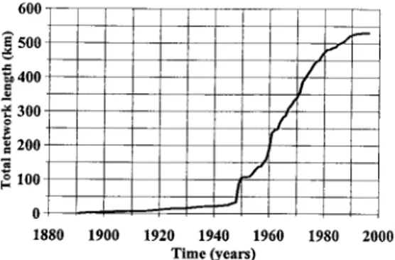
instal-lation, pipe length, soil type, and land use above pipe. More than 89% of pipe segments are under 300 m in length, with an average length of around 150 m. Figure 4 shows the evolution of total pipe length since the first pipes were laid in 1891. The municipality experienced a major growth in 1949, and urban development remained rapid until recent years.
Systematic recording of pipe breaks began in 1976. The observation period covers 21 years (1976–1996). There are some data missing for part of the year in 1978. Figure 5 pre-sents the evolution of the number of pipe breaks during the observation period. There is a net increase with time. The total number of breaks archived is 2289, but only 1719 breaks could be associated with a single pipe segment. These breaks all occurred on pipes and joints. Breaks on all other parts of the water pipe network, like fire hydrants and valves, are excluded from the analysis. In 1996, 163 pipe breaks occurred on the water pipe network. This corresponds globally to a break rate of 46 breaks per 100 km, which is considered high and a symptom of a degraded network according to a study done by McDonald et al. [1994] of the National Research Council of Canada. The average break rate in municipalities in Ontario (Canada) was estimated at 25 breaks per 100 km [Canada Mortgage and Housing Corporation, 1992] and was estimated at 13 breaks per 100 km in a sample of American cities [American Water Works Association, 1994].
4.2. Models Considered and Parameter Estimation Using Likelihood Functions
Table 2 presents the different models considered for the municipality of Chicoutimi. Four models were examined, with an increasing number of parameters. For each of these models the likelihood function was derived. A numerical method of optimization was used, namely, Powell’s algorithm [Press et al., 1988], to estimate the values of the calibration parameters. Validation of the likelihood function formulations and of the
Figure 4. Evolution of the total network length for the mu-nicipality of Chicoutimi.
Figure 5. Annual number of recorded breaks from 1976 to 1996 in the municipality of Chicoutimi.
Table 3. Example of Input File Needed to Estimate the Likelihood Function (Equation (15))
Pipe
Number InstallationYear of
Number of Breaks Observed Year of First Observed Break Time of Beginning of Observation Period (Tb)a Time of Analysis (Ta)a Time of First Observed Break (t1) 1 1950 1 1971 20 49 21 2 1972 0 䡠 䡠 䡠 0 18 䡠 䡠 䡠
aWe suppose, in this example, that the observation period begins in 1970 and that the time analysis is
method used for maximization were done by considering syn-thetic data generated with the proposed models. A sequence of pipe breaks was randomly generated for every pipe of a net-work. An “unrecorded” period was then assumed, and maxi-mization of the likelihood function was performed using infor-mation from the recorded period only. Resulting parameter values were compared to the actual ones used to generate the pipe break records, and they were found to be in close agree-ment.
After this verification the method was applied to Chicouti-mi’s data. At first, because of the complexity of the functions to optimize and the number of parameters (up to six), optimiza-tion was performed with only the pipe segments installed from the beginning of the recording period (1976–1996). For these pipe segments, “standard” survival analysis can be used, and therefore it was possible to verify that the likelihood functions of the different models considered were formulated appropriately.
4.3. Results
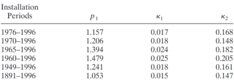
Tables 4 to 7 present the different values of the calibration parameters for all the models considered. Analyses were per-formed on pipe segments installed during these six periods: 1976 –1996, 1970 –1996, 1965–1996, 1960 –1996, 1949 –1996, and 1891–1996. The total number of pipe segments considered (including replaced and new pipes) in each case is 679, 1033, 1243, 1510, 2184, and 2404, respectively.
Tables 4–7 show that parameter values vary noticeably for different installation periods for all the models considered. Hence taking into account only pipe segments laid during the years covered by the observation period when estimating pa-rameter values will lead to significantly different results than when all pipe segments are used for the analysis. This suggests, as expected, that the installation period or another time-related factor (e.g., pipe material) has a strong impact on the probability of pipe failure.
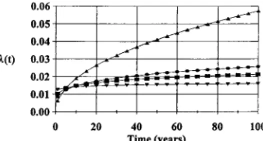
Figure 6 presents the hazard function of the Weibull distri-bution associated with the first break order for some installa-tion periods. Adding pipe segments installed in the 1960s
(in-stallation periods 1960–1996 and 1965–1996) has a strong influence on the shape of the hazard function: The risk of failure is much higher. It is important to note that the number of pipes installed during the 1960s (422 pipe segments) is comparable to the number of pipes installed in the 1950s (329 pipe segments) and in the 1970s (454 pipe segments). Since it is not only the weight of the number of pipes installed in the 1960s that can justify the higher failure risk, one must conclude that there is some unknown risk factor associated with this period. It could be related to some pipe characteristics or to some other factors such as the installation techniques used, the quality of pipe material, etc. The lowest risk of failure is found when all pipe segments are included (installation period 1891– 1996). The value of this function associated with all subsequent breaks is also higher for installation periods 1960–1996 and 1965–1996 (0.205 and 0.182, respectively) compared to all other installation periods (all values below 0.170). The lowest risk of subsequent breaks is also associated with the 1891–1996 installation period.
Comparing parameter values obtained for the different models (Tables 4–7), we observe that values of p1are
signif-icantly different from one. It should be noted that the expo-nential distribution is a special case of the Weibull distribution with p⫽ 1. Therefore the first break order (parameters p1and
1) is better described by a Weibull than an exponential
dis-tribution. The only exception is for period 1891–1996 for the Weibull-exponential (W-E) model (Table 4) since the p1value
is very close to 1. In that case an exponential distribution could be used. For the second break the p2values (Tables 6 and 7)
are often smaller than 1, meaning that the risk of failure de-creases with time, which would not be expected. However, in all cases but one (installation period 1891–1996 with the Weibull-Weibull-exponential model), the values of p2 cannot
be considered significantly different from 1. Therefore an ex-ponential distribution should be considered to model second breaks. In the case of exception the use of a Weibull distribu-tion is justified. Secdistribu-tion 5 presents a simple method to evaluate if exponential (W-W-E) and
Weibull-Table 5. Results of the W-E-E Model for Different Installation Periods Installation Periods p1 1 2 3 1976–1996 1.155 0.017 0.076 0.331 1970–1996 1.193 0.018 0.078 0.246 1965–1996 1.369 0.024 0.082 0.291 1960–1996 1.461 0.025 0.075 0.342 1949–1996 1.249 0.020 0.048 0.284 1891–1996 1.154 0.018 0.038 0.261
Table 7. Results of the W-W-E-E Model for Different Installation Periods Installation Periods p1 p2 1 2 3 4 1976–1996 1.157 0.922 0.017 0.070 0.166 0.521 1970–1996 1.184 0.991 0.018 0.079 0.130 0.374 1965–1996 1.342 0.993 0.023 0.084 0.140 0.407 1960–1996 1.404 1.008 0.025 0.081 0.119 0.494 1949–1996 1.243 0.955 0.020 0.061 0.071 0.438 1891–1996 1.123 0.917 0.018 0.055 0.049 0.420
exponential-exponential (W-E-E) models are significantly dif-ferent, permitting us to determine if a Weibull distribution is a better choice than an exponential distribution to model second break orders.
Is there a gain to be made by distinguishing between the second, third, and fourth break orders? Discriminating be-tween the second breaks and all subsequent breaks for the W-E-E model leads to significantly different values for the2
and3parameters compared to the2parameter of the W-E
model. However, parameter values for2of the W-E model
are roughly equal to the midvalue between the 2 and 3
parameter values of the W-E-E model, which is consistent with the fact that it is the average behavior that is modeled.
The same conclusion can be drawn for parameter values for 3of the W-W-E model compared to the3and4parameter
values of the Weibull-Weibull-exponential-exponential (W-W-E-E) model. With the W-W-E-E model the values of4(fourth
break order) are roughly 3 times higher than the values of parameter3(third break order). This could be symptomatic
of the fact that a group of pipe segments is largely responsible for the high number of subsequent breaks observed in recent years. This hypothesis should be further examined. Globally, we observe that as we have more breaks on a pipe segment, the probability of subsequent breaks increases (in Table 74 ⱖ
3ⱖ2). This has been reported by many authors [Clark et al.,
1982; Goulter and Kazemi, 1988]. Therefore there is a gain to be made by distinguishing between higher break orders as long as the number of pipes in the sample used to estimate the parameter values is statistically significant.
5. Discrimination Between W-W-E and W-E-E
Models
To evaluate if W-W-E and W-E-E models are significantly different, we verified the hypothesis p2 ⫽ 1 for the W-W-E
model. Given, a vector of parameters, the likelihood ratio R( ), which can be used for inference about , was calculated [Kalbfleisch and Prentice, 1980]. The statistic⫺2 log R(0) has
an asymptotic2distribution if ⫽
0, and an approximate
95% confidence interval for can be obtained. Refer to Kalb-fleisch and Prentice [1980] for details. Table 8 presents the minimum and maximum values of the 95% confidence interval for the p2 parameter of the W-W-E model.
When the value 1 for parameter p2is included in the 95%
confidence interval, the difference between a Weibull and an exponential distribution for the second break order is not sig-nificant at that confidence level. As presented in Table 8, the only case where the difference is significant is for the
installa-tion period 1891–1996. Also, since p2 is significantly smaller
than 1, it means that the hazard function decreases with time; thus, as time goes by, the probability of having a second pipe break on a given pipe segment decreases. This behavior is atypical, not consistent with the physical processes going on. Many hypotheses can be put forward. Among these it is pos-sible that the Weibull distribution is inappropriate to describe the second break order for older pipe segments or is inappro-priate to describe long-term behavior for these pipes. In order to verify this, a more precise analysis would be necessary, and that is beyond the scope of this paper. From this example we see that likelihood ratio is useful for comparing different types of models and for estimating if the available data make it possible to discriminate between them.
6. Summary and Conclusion
Rare are the municipalities that have recorded pipe breaks since the installation of the first pipes of their water pipe networks. In the case study presented here, the water pipe network of Chicoutimi is more than a century old, but the recorded pipe break history only covers 21 years (1976–1996). Different modeling strategies have been proposed in the liter-ature to describe the physical degradation of pipes with time. The most often used indicator of the physical degradation is the annual number of pipe breaks on the network. Many of the strategies used to model pipe breaks are based on statistical methods, especially survival analysis, to model pipe break be-havior and estimate the calibration parameters of those mod-els. Using “standard” survival analysis is not possible in the case where the recorded pipe break history does not cover the entire history of the water pipe network. The main reason is that the exact order of breaks that occurred during the obser-vation period is unknown. Survival analysis necessitates strat-ification of the times to failure depending on the exact break order so that each break order can be modeled with an appro-priate distribution. To use survival analysis, one would need to use only pipe segments that were installed during the obser-vation period, which is often only a small portion of the infor-mation available.
To model the evolution of the number of pipe breaks in a municipality with a brief recorded pipe break history, we have developed a rigorous approach inspired by survival analysis that permits the estimation of calibration parameters of a sta-tistical pipe break model while integrating all the available information, even though the pipe break history is only par-tially known for most pipe segments. The approach is based on likelihood functions that once maximized yield the optimal set of calibration parameters for the pipe break model considered. For the application in the municipality of Chicoutimi, four pipe
Figure 6. First-order break hazard function for the Weibull-exponential model. The different curves correspond to the following periods: (square) 1976–1996, (triangle) 1960–1996, (circle) 1949–1996, and (inverted triangle) 1891–1996.
Table 8. The 95% Confidence Interval for the p2
Parameter of the W-W-E Model for Different Installation Periods
Installation
Periods Average Minimum Maximum 1976–1996 0.924 0.692 1.195 1970–1996 0.999 0.825 1.196 1960–1996 1.043 0.915 1.185 1949–1996 0.968 0.853 1.107 1891–1996 0.779 0.711 0.924
dure enabled us to identify the 1960s as a critical period for Chicoutimi, since pipe segments installed during that time failed more rapidly than all other pipe segments. These results show that two or even three models of pipe break behavior should be used: one for pipe segments installed before the 1960s, one for those installed in the 1960s, and finally one for after the 1960s. There can be many possible explanations for the change of behaviors, but the most probable causes are related to the pipe materials and installation techniques used. Many authors have also observed that pipe breakage varies considerably between installation periods [e.g., Kleiner and Ra-jani, 1999] and thus should be taken into account by using different parameter sets (or even different distributions) for different installation periods.
It is also possible to assess, on a statistical basis, the relative performance of a Weibull distribution compared to an expo-nential distribution for a particular break order. An example was presented for the W-W-E and the W-E-E models. The likelihood ratio was used to calculate a 95% confidence inter-val on the inter-value of the p parameter which distinguishes a Weibull from an exponential distribution, since p ⫽ 1 in the latter case. In the presented example, we could conclude that the use of a Weibull distribution was only justified in the case of the 1891–1996 installation period, which represents the en-tire history of the water pipe network. In fact, it is interesting to note that very old pipe segments seem to have a much better break record than “younger” pipe segments. The reason for this behavior has yet to be elucidated.
The application of the developed approach to other munic-ipalities with brief recorded pipe break histories is currently being done. We are further investigating the impact of the duration of the recorded history on the quality of the results, and we plan to assess the impact of different risk factors (e.g., pipe material and pipe diameter) on the analysis.
Notation
f(t) probability density function.
n0 number of pipe segments that have not
failed during the observation period. nb total number of recorded breaks.
nt total number of pipe segments.
p “scale” parameter of the Weibull distribution. F(t) survival function.
L likelihood function.
P(␣, ; {tj}) probability to have␣ nonrecorded pipe breaks no matter when these breaks occurred and pipe breaks in the observation period at times {tj}. P⬘(; {tj}) probability to have pipe breaks in the
observation period at times {tj} no matter
Acknowledgments. This research was financed in part by the Min-istry of Municipal Affairs of Quebec. The authors would like to thank Normand Bouchard of the municipality of Chicoutimi for providing all the useful data and his expertise on the water pipe network and the reviewers of the paper for their useful comments.
References
American Water Works Association, An assessment of water distribu-tion systems and associated research needs, report, Am. Water Works Assoc. Res. Found., Denver, Colo., 1994.
Andreou, S. A., D. H. Marks, and R. M. Clark, A new methodology for modelling break failure patterns in deteriorating water distribution systems: Theory, Adv. Water Resour., 10(3), 2–10, 1987.
Canada Mortgage and Housing Corporation, Urban infrastructure in Canada, report, Ottawa, Ont., Canada, 1992.
Choate, P., and S. Walter, America in ruins, report, Counc. of State Plann. Agencies, Washington, D. C., 1981.
Clark, R. M., C. L. Stafford, and J. A. Goodrich, Water distribution systems: A spatial and cost evaluation, J. Water Resour. Plann.
Man-age., 108(3), 243–256, 1982.
Clark, R. M., R. G. Eilers, and J. A. Goodrich, Distribution system: Cost of repair and replacement, in Proceedings of the Conference on
Pipeline Infrastructure, edited by B. A. Bennett, pp. 428–440, Am.
Soc. of Civ. Eng., Reston, Va., 1988.
Cox, D. R., and D. Oakes, Analysis of Survival Data, 201 pp., Chapman and Hall, New York, 1994.
Desbiens, M.-E., La proble´matique des infrastructures urbaines: Sa re´solution par les voies de la me´thodologie et de la technologie, in
Annual Conference of the Canadian Society of Civil Engineering
(CSCE), edited by P. Labossie`re, R. Crysler, and D. T. Lau, pp. 37–43, Can. Soc. Civ. Eng., Montreal, Que., Canada, 1997. Eisenbeis, P., Mode´lisation statistique de la pre´vision des de´faillances
sur les conduites d’eau potable, in E´tudes du CEMAGREF, Se´r.
E´quip. Environ. 17, CEMAGREF, Bordeaux, France, 1994.
Goulter, I. C., and A. Kazemi, Spatial and temporal groupings of water main pipe breakage in Winnipeg, Can. J. Civ. Eng., 15, 91–97, 1988. Goulter, I. C., J. Davidson, and P. Jacobs, Predicting water-main breakage rates, J. Water Resour. Plann. Manage., 119(4), 419–436, 1993.
Herz, R. K., Ageing processes and rehabilitation needs of drinking water distribution networks, J. Water SRT Aqua, 45(5), 221–231, 1996.
Jacobs, P., and B. Karney, GIS development with application to cast iron water main breakage rate, paper presented at the 2nd Interna-tional Conference on Water Pipeline Systems, BHR Group Ltd., Edinburgh, Scotland, May, 1994.
Kalbfleisch, J. D., and R. L. Prentice, The Statistical Analysis of Failure
Time Data, Wiley Series in Probability and Mathematical Statistics,
321 pp., John Wiley, New York, 1980.
Karaa, F. A., and D. H. Marks, Performance of water distribution networks: Integrated approach, J. Performance Constr. Facil., 4(1), 51–67, 1990.
Kettler, A. J., and I. C. Goulter, An analysis of pipe breakage in urban water distribution networks, Can. J. Civ. Eng., 12, 286–293, 1985. Kleiner, Y., and B. B. Rajani, Using limited data to assess future
needs, J. Am. Water Works Assoc., 91(7), 47–62, 1999.
Kleiner, Y., B. J. Adams, and J. S. Rogers, Long-term planning meth-odology for water distribution system rehabilitation, Water Resour.
Res., 34(8), 2039–2051, 1998a.
Kleiner, Y., B. J. Adams, and J. S. Rogers, Selection and scheduling of rehabilitation alternatives for water distribution systems, Water
McDonald, S., L. Daigle, and G. Fe´lio, Re´seaux d’aqueduc et syste`mes d’e´gouts, report, Infrastruct. Lab., Inst. for Res. in Construct., Natl. Res. Counc. of Can., Ottawa, Ont., 1994.
Miller, R. G., Survival Analysis, 238 pp., John Wiley, New York, 1981. O’Day, D. K., R. Weiss, S. Chiavari, and D. Blair, Water main evalu-ation for rehabilitevalu-ation/replacement, report, Am. Water Works As-soc. Res. Found., Denver, Colo., 1986.
Pelletier, G., Impact du remplacement des conduites d’aqueduc sur le nombre annuel de bris, Ph.D. thesis, Inst. Natl. de la Rech. Sci., Sainte-Foy, Que´., Canada, 2000.
Press, W. H., B. P. Flannery, S. A. Teukolsky, and W. T. Vetterling,
Numerical Recipes in C, 735 pp., Cambridge Univ. Press, New York,
1988.
Shamir, U., and C. Howard, Analytic approach to scheduling pipe replacement, J. Am. Water Works Assoc., 71(5), 248–258, 1979. Siddiqui, S., and S. Mirza, Canadian municipal infrastructure—The
present state, in Annual Conference of the Canadian Society of Civil
Engineering (CSCE)—1st Transportation Specialty Conference, pp.
519–530, Can. Soc. of Civ. Eng., Montreal, Que., Canada, 1996. Villeneuve, J.-P., S. Duchesne, A. Mailhot, E. Musso, and G. Pelletier,
E´valuation des besoins des municipalite´s que´be´coises en re´fection et construction d’infrastructures d’eaux—Rapport final—INRS-Eau, research report, Inst. Natl. de la Rech. Sci., Sainte-Foy, Que´., Can-ada, 1998.
A. Mailhot, J.-F. Noe¨l, G. Pelletier, and J.-P. Villeneuve, Institut National de la Recherche Scientifique, INRS-Eau 2800, rue Einstein, C. P. 7500, Sainte-Foy, Que´bec, Canada C1V 4C7. (Alain_Mailhot@ inrs-eau.uquebec.ca)
(Received June 21, 1999; revised April 13, 2000; accepted June 6, 2000.)