HAL Id: cea-02623807
https://hal-cea.archives-ouvertes.fr/cea-02623807
Submitted on 26 May 2020HAL is a multi-disciplinary open access archive for the deposit and dissemination of sci-entific research documents, whether they are pub-lished or not. The documents may come from teaching and research institutions in France or abroad, or from public or private research centers.
L’archive ouverte pluridisciplinaire HAL, est destinée au dépôt et à la diffusion de documents scientifiques de niveau recherche, publiés ou non, émanant des établissements d’enseignement et de recherche français ou étrangers, des laboratoires publics ou privés.
Upgrade of apollo3® internal thermohydraulic feedback
model with THEDI, and application to a control-rod
ejection accident
Cyril Patricot, Roland Lenain, Dominic Caron
To cite this version:
Cyril Patricot, Roland Lenain, Dominic Caron. Upgrade of apollo3® internal thermohydraulic feed-back model with THEDI, and application to a control-rod ejection accident. M&C2019, ANS, Aug 2019, Portland, United States. �cea-02623807�
UPGRADE OF APOLLO3
®INTERNAL THERMOHYDRAULIC
FEEDBACK MODEL WITH THEDI, AND APPLICATION TO A
CONTROL-ROD EJECTION ACCIDENT
Cyril PATRICOT
1, Roland LENAIN
1, and Dominic CARON
11
DEN-Service d’études des réacteurs et de mathématiques appliquées (SERMA)
CEA, Université de Paris-Saclay, F-91191, Gif-sur-Yvette, France
cyril.patricot@cea.fr, roland.lenain@cea.fr, dominic.caron@cea.fr
ABSTRACT
In the frame of APOLLO3® project (new generation CEA code system for core physics
analysis based on deterministic neutron transport), it was decided to develop a new internal thermohydraulic feedback model: THEDI, a multi-1D, two-phase flow solver. This paper is dedicated to the presentation of the integration of THEDI in the APOLLO3® code. After a
brief presentation of THEDI and of its APOLLO3®’s interface, some code-to-code
verification cases are presented. First, APOLLO3®, using THEDI, is compared to CRONOS2
(a neutronic CEA code of the previous generation with its own feedback model) for steady-state and depletion calculations on a small PWR core. Then, APOLLO3® is compared to a
CRONOS2 – FLICA4 (a two-phase, four-equation three-dimensional thermohydraulic CEA code) coupling for control-rod ejection accidents, on a similar core. The objective of these comparisons is to verify the coupling between APOLLO3® neutronic solvers and THEDI.
They are therefore all made with identical models and data, and they all lead to very close results. Thanks to THEDI integration, APOLLO3®’s capabilities to model a nuclear reactor
core are improved. Thermohydraulic feedbacks can now be taken into account, in both steady-state and transient, for possibly diphasic flows.
KEYWORDS: APOLLO3®, THEDI, multi-physic coupling, control-rod ejection, CORPUSSALOME
1. INTRODUCTION
Data used in neutron transport calculations vary with the temperatures and the densities of media, issued from thermohydraulics. In the same time, thermohydraulics needs the power distribution in the core, which is provided by neutronics. As a consequence, it is mandatory to couple these two physics in order to correctly compute a nuclear reactor.
The strategy followed by CEA to address this issue is twofold. On the one hand, specialized codes are developed, for example APOLLO3® [1] (new generation CEA code system for core physics analysis
based on deterministic neutron transport) and FLICA4 [2] (a two-phase, four-equation three-dimensional thermohydraulic code), coupled in the multi-physics platform CORPUSSALOME [3] (“external” coupling).
On the other hand, and complementarily with the previous approach, neutronic codes dedicated to core calculations often have their own simplified thermohydraulic model (“internal” coupling). It simplifies routine nuclear reactor calculations which do not always need a very accurate thermohydraulic model. In
that respect, CRONOS2 [4], the production CEA deterministic neutron transport code, dedicated to PWR core analysis, uses THERMOC, a three-equations multi-1D model.
In the frame of APOLLO3® project, it was decided to develop a new thermohydraulic model for internal
coupling: THEDI (THErmohydraulique DIphasique) [5]. THEDI is a multi-1D, two-phase flow solver. It improves the modeling, compared to THERMOC, thanks to a four-equation model (instead of three), and to some new system modeling capabilities. Moreover, THEDI is written in C++ (instead of FORTRAN) with the objective to improve code flexibility, maintainability and performance. It was also conceived as an independent tool in order to allow future sharing with other neutronic codes (like the Monte Carlo code TRIPOLI-4® [6]). It is linked as an external library by client codes.
The integration of THEDI in APOLLO3®, its coupling with neutron transport solvers and the new abilities
provided to APOLLO3® by this work are presented in this paper. Some verification cases are also
presented: comparisons with CRONOS2, using THERMOC or coupled with FLICA4 within the multi-physics platform CORPUSSALOME, for control-rod ejection accidents on a small PWR core.
2. THEDI MODELING
THEDI is presented in a dedicated paper [5]. Some elements are recalled here.
The main thermohydraulic model is one-dimensional and treats a four-equation system composed of total mass conservation, vapor mass conservation, total motion equation and total internal energy conservation. The core is therefore divided into separated 1D channels sharing consistent boundary conditions: this is the “multi-1D approach”, already used by THERMOC. Each mesh of each thermohydraulic channel can contain several solid objects, such as fuel rods. THEDI computes the temperature distribution in each of them, by solving one-dimensional heat transfer diffusion equation. THEDI is also able to compute the power evolution during a transient by solving the neutronic point kinetic equations.
THEDI is, at the moment, able to model light water and sodium-cooled reactors in normal and accidental (with possible two phase flow) conditions.
3. INTEGRATION OF THEDI IN APOLLO3®
APOLLO3® is a multipurpose neutronic code which permits to carry out lattice calculations
(self-shielding and flux calculations used to produce multi-parametrized cross-section libraries) up to full core calculations (from multi-parametrized cross-section libraries) with several solvers using different angular approximation (Sn, PN, SPN and diffusion).
APOLLO3® has integrated THEDI as its internal thermohydraulic module since September 2018. An
interface to THEDI has been developed in APOLLO3®, based on APOLLO3® data model, to initialize
THEDI module (definition of a coherent geometry between neutronics and thermohydraulics) and to manage coupled calculations (it transfers power to thermohydraulics and temperatures and densities to neutronics). The interface proposed allows specifying a 2D-1D thermohydraulic grid, in which each column is a hydraulic channel. This grid forms a 3D unstructured mesh where each region can receive specific hydraulic properties. Each mesh of the hydraulic grid can receive solid objects. The assignment of solid objects within each hydraulic region can be done with a spatial distribution over the mesh allowing modeling every fuel rod distinctly in the core. This forms an unstructured solid object grid. The inputs for THEDI’s interface are 3D power distributions for each grid: hydraulic and solid object ones. THEDI outputs are given on the different grids. All the quantities exchanged are based on APOLLO3® data model, allowing easy use in APOLLO3® framework. Consequently, the final user does
not need to know THEDI’s data model to run coupled calculation as the interface is in charge of format conversion between APOLLO3® data model and THEDI’s. Moreover, coupling calculation can be carried
out with every neutronic solver of APOLLO3® without any additional effort.
4. COMPARISON WITH CRONOS2
In order to verify the integration of THEDI in APOLLO3®, a comparison has been made with CRONOS2.
CRONOS2 is the CEA neutron transport code, dedicated to core scale PWR applications, of the previous code generation. CRONOS2 is particularly relevant for this code-to-code benchmark because its neutron diffusion solver (MINOS) has been ported in APOLLO3®. Neutronics results should therefore be in very
good agreements (as long as diffusion solver is used in APOLLO3®).
CRONOS2 has its own thermohydraulic module, THERMOC. Like THEDI, THERMOC is multi-1D. However, THERMOC’s thermohydraulic model is three-equation instead of four (no vapor mass conservation equation). Correlations can be used in order to compute the gas volume fraction. Vapor and liquid have the same velocity. Only steady-state THERMOC calculations are presented in this paper. 4.1. Benchmark Definition
A small PWR core, with 32 assemblies (Fig. 3 shows a sketch of the core), is considered for this benchmark. Each assembly has a reduced height, but is otherwise representative of a standard PWR. This core is not functional and is only used for numerical benchmarks. The comparison is made first for a beginning of life steady-state calculation, and then for a simple depletion calculation.
Neutron transport computations are made, by the two neutronic codes, in diffusion with 4 energy groups, on homogenous rod-cell mesh. Cross-sections were generated by APOLLO2 [7] with Method Of Characteristic calculations [8] and 281 energy groups [9]. No control-rods are considered here.
Thermohydraulic computations are made with one channel per assembly. Fuel temperatures are calculated on a mean fuel rod per assembly for the code-to-code comparisons. APOLLO3® results with the
calculation of all fuel rods are also included for physical analysis. Exchanged data are, here, always pin averaged. Rowland formula [10] is used to compute the fuel effective temperature, used by neutronic solvers, from the radial temperature distribution calculated in fuel pellets by THERMOC or THEDI. The axial mesh is shared by all physics, and is made of meshes of about 3 cm.
4.2. Beginning of Life Steady-State
Without feedback, APOLLO3® and CRONOS2 both give a reactivity of 14718 pcm and a 3D power
peaking factor of 2.945. Results with feedback are given in the Table I and show a good agreement between codes. The effect on reactivity of the calculation of every fuel rod is small here, about 17 pcm.
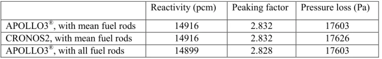
Table I. Reactivity and pressure loss from APOLLO3® and CRONOS2 in steady-state.
Reactivity (pcm) Peaking factor Pressure loss (Pa) APOLLO3®, with mean fuel rods 14916 2.832 17603
CRONOS2, with mean fuel rods 14916 2.832 17626
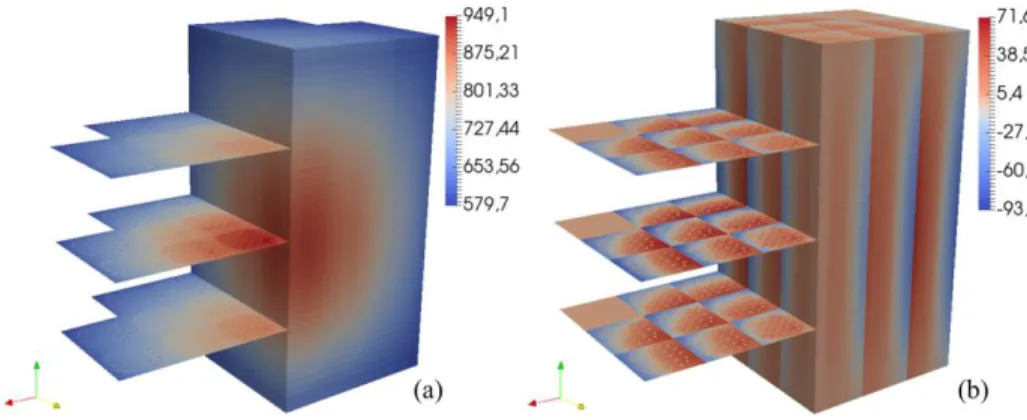
Fig.1.a shows the fuel effective temperature from APOLLO3® calculation with every fuel rods, and
Fig.1.b shows the map of the difference of fuel effective temperature between calculations with one mean fuel rod per assembly and with every fuel rods in the core. In Fig.1.b, the effect visible in each assembly is directly linked to the gradient of power. This effect is found to be quite important here, up to 100 K, although the impact on the reactivity, visible in Table I, is small. This new capability of APOLLO3®
improves its ability to compute local phenomena.
Figure 1. (a) Fuel effective temperature (K). (b) Fuel effective temperature difference (K) between one mean fuel rod per assembly and the calculation of every fuel rods.
4.3. Depletion
A very simple depletion calculation is done here: macroscopic cross-sections (generated by APOLLO2) are parametrized with respect to the local burnup. At the core scale, the burnup is computed at each time step and is used to update the cross-sections. The process is repeated until a criterion is reached (here, a given mean burnup). No depletion chain is thus needed at the core level. When a thermohydraulic feedback is used, a coupled computation is made at each time-step, instead of a simple neutronic one. During the depletion, the multiplication factor varies from 1.17 to 0.92 (that is to say, a variation of about 25,000 pcm). An initial reactivity drop of about 2,500 pcm is foreseen, corresponding to absorbing fission product (135Xe) production. The differences in reactivity of different calculations are given in Fig. 2 (the
first two curves are repeated with an adapted scale on the right). The effect of the thermohydraulic feedback varies from 200 pcm to 600 pcm here. The agreement between APOLLO3® and CRONOS2
with thermohydraulic feedback is very good: the difference in reactivity is always less than 30 pcm. The reactivity effect of the calculation of every fuel rod is pretty constant during the depletion.
5. COMPARISON WITH CORPUSSALOME
APOLLO3® can model multi-physic transients by coupling THEDI with kinetic neutron transport solvers.
In order to verify this new APOLLO3®’s capability, a comparison has been made with CORPUSSALOME,
for control-rod ejection accidents on a small PWR core.
CORPUSSALOME is a coupling platform developed by CEA for reactor physics analysis. It is based on
Salome, an open source platform which provides, among others, generic tools for code coupling. The main CEA codes for core physics analysis can be coupled within CORPUSSALOME:
- Core neutronics can be computed by either CRONOS2 or APOLLO3®, - Core thermohydraulics can be computed by FLICA4,
- Reactor system computations can be done by either CATHARE2 [11] or CATHARE3 [12], - Fuel physics simulations can be performed by ALCYONE2 [13].
CORPUSSALOME was first made for PWR applications, but fast reactor capabilities are under-development.
In the following, CORPUSSALOME isused to couple CRONOS2 and FLICA4. As already mentioned,
CRONOS2 is chosen because its diffusion solver is identical to APOLLO3®’s one. The time-schemes
used for kinetics calculations are, here, nevertheless slightly different. Similarly, the set of equations solved by THEDI and FLICA4 are the same (but the solver implementations are different). They should thus provide a similar answer to the same problem. FLICA4 was already used to verify THEDI in [5]. 5.1. Benchmark Definition
For this benchmark, a core similar to the one used in section 4 is considered. The core geometry is the same, but the detailed compositions are different. The following calculations are always made with a core at beginning of life.
In order to have quick calculations, we use a coarser discretization, identical in both APOLLO3® and CORPUSSALOME. Neutronics is computed with diffusion and 2 energy groups, on a homogenous assembly
mesh. Cross-sections were generated by APOLLO2 using the process presented in the previous section. Thermohydraulic computations are made with one channel per assembly. Fuel temperatures are calculated on one mean fuel rod per assembly. The axial mesh is common and fixed, and meshes are about 3cm. The mass flow in each assembly is imposed (the same for all assemblies), and does not vary during the accidents. The core pressure drop is therefore not precisely defined.
For the code-to-code benchmark, FLICA4 model used in CORPUSSALOME calculations uses “closed”
channels in order to reproduce the multi-1D modelling of THEDI. However, CORPUSSALOME results with
open channels in FLICA4 are also included for physical analysis. It is important to note that a 3D thermohydraulic best estimate calculation would not only use open channels, but also refined radial mesh. Two control-rod ejection accidents are considered:
1. The core is initially at a full power steady-state (100 MW), with the control-rod 1 fully inserted (see Fig. 3). This control-rod is then ejected in 0.1 s. Sub-cooled vapor production correlations are not used, the transient is strictly monophasic.
2. The core is initially at a full power steady-state (100 MW), with the four control-rods fully inserted (see Fig. 3). The control-rod number 1 is then ejected in 0.1 s. Two-phase flows with high void fractions are observed during this transient.
In both cases, the initial reactivity is made equal to 0 by dividing fission cross-sections by the multiplication factor of the initial steady-state.
Figure 3. Control-rod position.
Both transients are computed with 10−4 s time-steps for both neutronics and thermohydraulics. An
explicit time-scheme is used for coupled variables. 5.2. Ejection Scenario 1
5.2.1. Steady-state
The main results on the initial steady-state are given in Table II. APOLLO3® and CORPUS are in perfect agreement. The ejected control-rod weight is about 1 $ here. The opening of channels in CORPUS has no impact (the forced convection is dominant at the assembly scale here).
Table II. Main results on the initial steady-state of the 1st ejection.
Reactivity (pcm) Peak power Ejected control-rod weight (pcm)
APOLLO3® 17091 2.733 800 (0.99 $)
CORPUS 17092 2.733 800 (0.99 $)
CORPUS with open channels 17092 2.733 800 (0.99 $)
The initial power map (from either APOLLO3® or CORPUS) is given in Fig. 4. On the left, a 2D slice of the middle of the core is shown, and, on the right, the axial power distribution in the hot fuel assembly is given. The control-rod position is indicated with a yellow square. The impact of the control-rod on the power distribution is clearly visible.
5.2.2. Transient
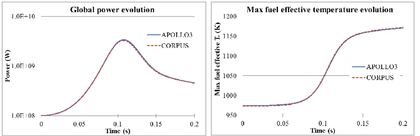
The global power and max fuel effective temperature evolutions are given in Fig. 5, and the main results are repeated in Table III. A very good agreement is found between APOLLO3® and CORPUSSALOME. The opening of channels in CORPUS has no impact on this transient. We recall that there is no sub-cooled vapor production here, this transient is strictly monophasic.
Figure 4. Initial power map of the 1st ejection.
Figure 5. Total power (left) and max fuel effective temperature (right) evolutions during 1st ejection.
Table III. Main results of the 1st ejection.
Max power (W) Max fuel effective temperature (K)
APOLLO3 3.41 109 1171
CORPUS 3.28 109 1172
CORPUS with open channels 3.28 109 1172
In order to analyze the local difference during the transient, the maximum and average differences between the power maps renormalized to the same value at each time step are given in Fig. 6. These quantities are given as a ratio to the average power. They are defined in equations (1) to (3), with 𝑃𝑖 being
the power density of mesh 𝑖 for each time step, and 𝑉𝑖 the volume of mesh 𝑖. 𝑃𝑎𝑣𝑒𝑟𝑎𝑔𝑒=∑ 𝑃𝑖 𝑖𝑉𝑖 ∑ 𝑉𝑖 𝑖 , (1) 𝑀𝑎𝑥 𝑑𝑖𝑓𝑓𝑒𝑟𝑒𝑛𝑐𝑒 = max𝑖|𝑃𝑖𝐶𝑂𝑅𝑃𝑈𝑆 𝑃𝑎𝑣𝑒𝑟𝑎𝑔𝑒𝐴𝑃𝑂𝐿𝐿𝑂3 𝑃𝑎𝑣𝑒𝑟𝑎𝑔𝑒𝐶𝑂𝑅𝑃𝑈𝑆 − 𝑃𝑖 𝐴𝑃𝑂𝐿𝐿𝑂3| / 𝑃 𝑎𝑣𝑒𝑟𝑎𝑔𝑒𝐴𝑃𝑂𝐿𝐿𝑂3 (2) 𝐴𝑣𝑒𝑟𝑎𝑔𝑒 𝑑𝑖𝑓𝑓𝑒𝑟𝑒𝑛𝑐𝑒 =∑ 𝑉1 𝑖 𝑖 ∑ 𝑉𝑖|𝑃𝑖 𝐶𝑂𝑅𝑃𝑈𝑆 𝑃𝑎𝑣𝑒𝑟𝑎𝑔𝑒𝐴𝑃𝑂𝐿𝐿𝑂3 𝑃𝑎𝑣𝑒𝑟𝑎𝑔𝑒𝐶𝑂𝑅𝑃𝑈𝑆 − 𝑃𝑖 𝐴𝑃𝑂𝐿𝐿𝑂3| 𝑖 ⁄𝑃𝑎𝑣𝑒𝑟𝑎𝑔𝑒𝐴𝑃𝑂𝐿𝐿𝑂3 (3)
It can be seen that local differences are always small during the transient, and stay below 1.5%. This shows the good agreement between APOLLO3® and CORPUSSALOME on local power. The shape of the max difference curve may be due to differences in the time-integration techniques of the neutron diffusion solvers (in particular for precursor concentrations from 0.13 s).
Figure 6. Power map max and average differences during 1st ejection
The final power map (from either APOLLO3® or CORPUS) is given in Fig. 7 (slice in the middle of the core on the left and the axial distribution in the assembly with the power peak on the right). It is interesting to note that the final power map is not perfectly symmetric. The power is maximized nearby the initial position of the control-rod: the core was initially cooler there, leading to a more reactive zone. A longer calculation would obviously lead a symmetric final state.
Figure 7. Final power map of 1st ejection.
5.3. Ejection Scenario 2 5.3.1. Steady-state
The main results on the initial steady-state are given in Table IV. Here again, APOLLO3® and CORPUS are in perfect agreement, and the opening of channels has no impact. The ejected control-rod weight is very strong here, about 2 $. The reader has to keep in mind that this reactivity is not injected instantaneously: the control-rod is ejected in 0.1 s (as in the 1st ejection).
The initial power map (from either APOLLO3® or CORPUS) is given in Fig. 8, and is perfectly symmetric. Yellow squares indicate the control-rod positions.
Table IV. Main results on the initial steady-state of the 2nd ejection.
Reactivity (pcm) Peak power Ejected control-rod weight (pcm)
APOLLO3 13457 2.694 1648 (2.05 $)
CORPUS 13457 2.694 1648 (2.05 $)
CORPUS with open channels 13457 2.694 1648 (2.05 $)
Figure 8. Initial power map of the 2nd ejection.
5.3.2. Transient
The global power, max fuel effective temperature and max void fraction evolutions are given in Fig. 9 and 10, and the main results are repeated in Table V. A good agreement is found between APOLLO3® and CORPUSSALOME. Some little differences can be suspected in the treatment of diphasic flow between FLICA4 and THEDI. The opening of channels in CORPUS has a small impact on the results here.
Figure 9. Total power (left) and max fuel effective temperature (right) evolutions during 2nd
Figure 10. Max void fraction evolutions during 2nd ejection.
Table V. Main results of the 2nd ejection. Max power (W) Max fuel effective
temperature (K)
Max void fraction
APOLLO3 3.98 1010 1830 0.40
CORPUS 3.78 1010 1827 0.38
CORPUS with open channels
3.75 1010 1816 0.44
The maximum and average differences between the normalized power maps are given in Fig. 11 (these quantities are defined in equations (1) to (3)). The differences are higher than in the first ejection, but are still small: the average power difference reach a maximum of about 1.5%, while the maximum difference goes up to 12% at the end of the transient. These differences are probably due to thermohydraulic effects.
Figure 11. Power map max and average differences during 2nd ejection.
Final power and void fraction maps (from APOLLO3® on the left of figures and CORPUS on the right) are given in Fig. 12 and 13. Yellow squares indicate the control-rod positions. The power maps are given on a slice in the middle of the core, together with the axial distribution in the assembly with the maximum power. The void fraction maps are given on a slice at the height of the maximum void fraction, together with the axial distribution in the assembly with the maximum void fraction.
The shapes of these maps are in good agreement, although the differences in the power distribution are maximize at this time (end of transient) according to Fig. 11. The small difference in total power and maximum void fraction, visible in Fig. 9 and 10 is visible in the color shift of these maps. The final power map is here clearly shifted to the bottom of the core. This is due to the heating of the upper part of the core, and is thus a good example of the impact of thermohydraulic convection on neutronics.
Figure 12. Final power maps of the 2nd ejection (left: APOLLO3®, right: CORPUS)
Figure 13. Final void fraction maps of the 2nd ejection (left: APOLLO3®, right: CORPUS)
6. CONCLUSIONS
This paper presents the integration of THEDI in APOLLO3®. THEDI is a thermohydraulic solver
developed to enhance the internal thermohydraulic models of CEA neutronic codes. A more detailed presentation of THEDI can be found in [5].
This integration is verified by a comparison with CRONOS2 in steady-state and CORPUSSALOME (used to
couple CRONOS2 and FLICA4) in transient.
CRONOS2 is a CEA neutron transport code of the previous generation. It also has an internal thermohydraulic module, THERMOC. The comparison is made for coupled neutronic and thermohydraulic steady-state and depletion calculations, on a small PWR core. Models and data are the same (in particular, only monophasic flows are considered), leading to very close results.
CORPUSSALOME is a CEA coupling platform dedicated to reactor physics analysis. Main CEA codes for
reactor physics can be coupled within CORPUSSALOME. A coupling between CRONOS2 and FLICA4 (a
two-phase, four-equation thermohydraulic code) is used in this case. Two rod-ejection accidents are considered. Coupled neutronic and thermohydraulic kinetic calculations are compared. Here again, models and data are the same, and results found by APOLLO3® and CORPUSSALOME are very similar.
This time, strongly diphasic flows are studied.
Thanks to THEDI integration, APOLLO3®’s capabilities to model nuclear reactor cores are improved.
Thermohydraulic feedbacks can now be taken into account, in both steady-state and transient, for possibly diphasic flows and with local fuel rod temperature calculation. However, THEDI is a simplified tool, and should be substituted by specialized thermohydraulic codes when a multi-1D four-equation model is not adequate.
ACKNOWLEDGMENT
The authors wish to thank Framatome & EDF for financial support on APOLLO3®.
REFERENCES
1. D. Schneider, et al., “APOLLO3®: CEA/DEN deterministic multi-purpose code for reactor physics analysis”, Proceedings of PHYSOR2016, Sun Valley, Idaho, USA, May 1-5 (2016).
2. I. TOUMI, et al., “FLICA-4: a three-dimensional two-phase flow computer code with advanced numerical methods for nuclear applications”, Nuclear Engineering and Design 200(1-2), pp. 139-155 (2000).
3. J.-C. Le Pallec, K. Mer-Nkonga and N. Crouzet, “Neutronics/fuel thermomechanics coupling in the framework of a REA (Rod Ejection Accident) transient scenario calculation”, Proceedings of PHYSOR2016, Sun Valley, Idaho, USA, May 1-5 (2016).
4. J. J. Lautard, S. Loubière, and C. Fedon-Magnaud, “CRONOS: a modular computational system for neutronic core calculations”. Proceedings of IAEA, Cadarache, France, September 10-14 (1992). 5. C. Patricot, “THEDI: a multi-1D two-phase flow solver for neutronic codes”, Proceedings of
ICAPP2019, Juan-les-Pins, France, May 12-15 (2019).
6. E. Brun, et al., “Tripoli-4®, CEA, EDF and AREVA reference Monte Carlo code”, Proceedings of SNA + MC 2013, Paris, France, October 27-31 (2013).
7. R. Sanchez, et al. "APOLLO2 year 2010." Nuclear Engineering and Technology 42(5), pp. 474-499 (2010).
8. S. Santandrea, et al., “A neutron transport characteristics method for 3D axially extruded geometries coupled with a fine group self-shielding environment,” Nuclear Science and Engineering 186(3), pp. 239-276 (2017).
9. A. Santamarina, and N. Hfaiedh, “The SHEM energy mesh for accurate fuel depletion and BUC calculations”, Proceedings of ICNC2007, St Petersburg, Russia (2007).
10. G. Rowlands, “Resonance absorption and non-uniform temperature distributions” J. Nuclear Energy, Pts. A & B. Reactor Sci. and Technol. 6 (1962).
11. G. Geffraye, et al. “CATHARE 2 V2. 5_2: a single version for various applications” Nuclear Engineering and Design 241(11), pp. 4456-4463 (2011).
12. P. Emonot, et al. “CATHARE-3: A new system code for thermal-hydraulics in the context of the NEPTUNE project” Nuclear Engineering and Design 241(11), pp. 4476-4481 (2011).
13. V. Marelle, et al. “Validation of PLEIADES/ALCYONE 2.0 fuel performance code” Proceedings of Water Reactor Fuel Performance Meeting, Jeju Island, Korea, September 10-14 (2017).