Collective motion of self-propelled particles interacting without cohesion

HAL Id: hal-00517100

https://hal.archives-ouvertes.fr/hal-00517100

Submitted on 31 Jul 2014

HAL is a multi-disciplinary open access

archive for the deposit and dissemination of

sci-entific research documents, whether they are

pub-lished or not. The documents may come from

teaching and research institutions in France or

abroad, or from public or private research centers.

L’archive ouverte pluridisciplinaire HAL, est

destinée au dépôt et à la diffusion de documents

scientifiques de niveau recherche, publiés ou non,

émanant des établissements d’enseignement et de

recherche français ou étrangers, des laboratoires

publics ou privés.

without cohesion

Hugues Chaté, Francisco Ginelli, Guillaume Grégoire, Franck Raynaud

To cite this version:

Hugues Chaté, Francisco Ginelli, Guillaume Grégoire, Franck Raynaud. Collective motion of

self-propelled particles interacting without cohesion. Physical Review E : Statistical, Nonlinear, and Soft

Matter Physics, American Physical Society, 2008, 77, pp.046113. �hal-00517100�

Collective motion of self-propelled particles interacting without cohesion

Hugues Chaté and Francesco Ginelli

CEA—Service de Physique de l’État Condensé, Centre d’Etudes de Saclay, 91191 Gif-sur-Yvette, France

Guillaume Grégoire

Matière et Systèmes Complexes, CNRS UMR 7057, Université Paris–Diderot, Paris, France

Franck Raynaud

CEA—Service de Physique de l’État Condensé, Centre d’Etudes de Saclay, 91191 Gif-sur-Yvette, France and Matière et Systèmes Complexes, CNRS UMR 7057, Université Paris–Diderot, Paris, France

共Received 12 December 2007; published 18 April 2008兲

We present a comprehensive study of Vicsek-style self-propelled particle models in two and three space dimensions. The onset of collective motion in such stochastic models with only local alignment interactions is studied in detail and shown to be discontinuous共first-order-like兲. The properties of the ordered, collectively moving phase are investigated. In a large domain of parameter space including the transition region, well-defined high-density and high-order propagating solitary structures are shown to dominate the dynamics. Far enough from the transition region, on the other hand, these objects are not present. A statistically homogeneous ordered phase is then observed, which is characterized by anomalously strong density fluctuations, superdif-fusion, and strong intermittency.

DOI:10.1103/PhysRevE.77.046113 PACS number共s兲: 05.65.⫹b, 64.70.qj, 87.18.Gh

I. INTRODUCTION

Collective motion phenomena in nature have attracted the interest of scientists and other authors for quite a long time 关1兴. The question of the advantage of living and moving in groups, for instance, is a favorite one among evolutionary biologists 关2兴. In a different perspective, physicists are mostly concerned with the mechanisms at the origin of col-lective motion, especially when it manifests itself as a true, nontrivial, emerging phenomenon, i.e., in the absence of some obvious cause like the existence of a leader followed by the group, a strong geometrical constraint forcing the dis-placement, or some external field or gradient felt by the whole population. Moreover, the ubiquity of the phenom-enon at all scales, from intracellular molecular cooperative motion to the displacement in groups of large animals, raises, for physicists at least, the question of the existence of some universal features possibly shared among many different situations.

One way of approaching these problems is to construct and study minimal models of collective motion: if universal properties of collective motion do exist, then they should appear clearly within such models and thus could be effi-ciently determined there, before being tested for in more elaborate models and real-world experiments or observa-tions. Such is the underlying motivation of recent studies of collective motion by a string of physicists 关3–8兴. Among them, the group of Vicsek has put forward what is probably the simplest possible model exhibiting collective motion in a nontrivial manner.

In the Vicsek model关9兴, point particles move off lattice at constant speed v0, adjusting their direction of motion to that of the average velocity of their neighbors, up to some noise term accounting for external or internal perturbations 共see below for a precise definition兲. For a finite density of par-ticles in a finite box, perfect alignment is reached easily in

the absence of noise: in this fluctuationless collective motion, the macroscopic velocity equals the microscopic one. On the other hand, for strong noise particles are essentially nonin-teracting random walkers and their macroscopic velocity is zero, up to statistical fluctuations.

Vicsek et al. showed that the onset of collective motion occurs at a finite noise level. In other words, there exists, in the asymptotic limit, a fluctuating phase where the macro-scopic velocity of the total population is, on average, finite. Working mostly in two space dimensions, they concluded, on the basis of numerical关5,9兴 simulations, that the onset of this ordered motion is well described as a novel nonequilibrium continuous phase transition leading to long-range order, at odds with equilibrium where the continuous XY symmetry cannot be spontaneously broken in two space dimensions and below关10兴. This brought support to the idea of universal properties of collective motion, since the scaling exponents and functions associated with such phase transitions are ex-pected to bear some degree of universality, even out of equi-librium.

The above results caused a well-deserved stir and prompted a large number of studies at various levels 关3,4,6–8,11–37兴. In particular, two of us showed that the on-set of collective motion is in fact discontinuous关38兴, and that the original conclusion of Vicsek et al. was based on numeri-cal results obtained at too small sizes关5,9兴. More recently, the discontinuous character of the transition was challenged in two publications, one by Vicsek and co-workers关39兴 and another by Aldana et al.关40兴.

Here, after a definition of the models involved共Sec. II兲, we come back, in Sec. III, to this central issue and present a rather comprehensive study of the onset of collective motion in Vicsek-style models. In Sec. IV, we describe the ordered, collective motion phase. Section V is devoted to a general discussion of our results together with some perspectives. Most of the numerical results shown were obtained in two

space dimensions, but we also present three-dimensional re-sults. Wherever no explicit mention is made, the default space dimension is 2. Similarly, the default boundary condi-tions are periodic in a square or cubic domain.

II. THE MODELS A. Vicsek model: Angular noise

Let us first recall the dynamical rule defining the Vicsek model关9兴. Point particles labeled by an integer index i move off lattice in a space of dimension d with a velocity vជi of

fixed modulus v0=兩vជi兩. The direction of motion of particle i

depends on the average velocity of all particles共including i兲 in the spherical neighborhood Siof radius r0 centered on i. The discrete-time dynamics is synchronous: the direction of motion and the positions of all particles are updated at each time step ⌬t, in a driven, overdamped manner,

vជ_i共t + ⌬t兲 = v₀共R_␩ⴰ␽兲

冉

兺

j僆Si

vជ_j共t兲

冊

where␽ is a normalization operator关␽共wជ兲=wជ/兩wជ兩兴 and R_␩ performs a random rotation uniformly distributed around the argument vector: in d = 2, R␩vជ is uniformely distributed

around vជ inside an arc of amplitude 2␲␩; in d = 3, it lies in the solid angle subtended by a spherical cap of amplitude 4␲␩and centered around vជ. The particle positions rជiare then

simply updated by streaming along the chosen direction as in

r

ជi共t + ⌬t兲 = rជi共t兲 + ⌬tvជi共t + ⌬t兲. 共2兲

Note that the original updating scheme proposed by Vicsek

et al.in关9兴 defined the speed as a backward difference, al-though we are using a forward difference. The simpler up-dating above, now adopted in most studies of Vicsek-style models, is not expected to yield different results in the asymptotic limit of infinite size and time.

B. A different noise term: Vectorial noise

The “angular” noise term in the model defined above can be thought of as arising from the errors committed when particles try to follow the locally averaged direction of mo-tion. One could argue, on the other hand, that most of the randomness stems from the evaluation of each interaction between particle i and one of its neighbors, because, e.g., of perception errors or turbulent fluctuations in the medium. This suggests the replacement of Eq.共1兲 by

vជ_i共t + ⌬t兲 = v₀␽

冉

兺

j僆Si

vជ_j共t兲 +␩N_i␰ជ

冊

where ␰ជ is a random unit vector and Ni is the number of

particles in Si. It is easy to realize that this “vectorial” noise

acts differently on the system. While the intensity of angular noise is independent of the degree of local alignment, the influence of the vectorial noise decreases with increasing lo-cal order.

C. Repulsive force

In the original formulation of the Vicsek model as well as in the two variants defined above, the only interaction is

alignment. In a separate work 关22兴, we introduced a two-body repulsion or attraction force, to account for the possi-bility of maintaining the cohesion of a flock in an infinite space 共something the Vicsek model does not allow兲. Here, we only study models without cohesion. Nevertheless, we have considered, in the following, the case of a pairwise repulsion force, to estimate in particular the possible influ-ence of the absinflu-ence of volume exclusion effects in the basic model, which leaves the local density actually unbounded. We thus introduce the short ranged, purely repulsive interac-tion exerted by particle j on particle i:

f

ជ_ij= − eជij⫻关1 + exp共兩rជj− rជi兩/rc− 2兲兴

−1

, 共4兲

where eជijis the unit vector pointing from particle i to j and

rc⬍ r0 is the typical repulsion range. Equations共1兲 and 共3兲 are then respectively generalized to

vជ_i共t + ⌬t兲 = v₀共R_␩ⴰ␽兲

冉

兺

兺

冊

冉

兺

兺

冊

D. Control and order parameters

The natural order parameter for our polar particles is sim-ply the macroscopic mean velocity, conveniently normalized by the microscopic velocity v0,

␸ជ共t兲 = 1

v₀具vជi共t兲典i

, 共7兲

where具·典istands for the average over the whole population.

Here, we mostly consider its modulus␸共t兲=兩␸ជ共t兲兩, the scalar

order parameter.

In the following, we set, without loss of generality, ⌬t = 1 and r0= 1, and express all time and length scales in terms of these units. Moreover, the repulsive force will be studied by fixing rc= 0.127 and␤= 2.5.

This leaves us with two main parameters for these mod-els: the noise amplitude␩and the global density of particles

␳. Recently, the microscopic velocity v0 has been argued to play a major role as well关39兴. All three parameters 共␩,␳, and

v₀兲 are considered below.

III. ORDER-DISORDER TRANSITION AT THE ONSET OF COLLECTIVE MOTION

As mentioned above, the original Vicsek model attracted a lot of attention mostly because of the conclusions drawn from the early numerical studies关5,9兴: the onset of collective motion was found to be a novel continuous phase transition spontaneously breaking rotational symmetry. However, it was later shown in关38兴 that beyond the typical sizes consid-ered originally the discontinuous nature of the transition emerges, irrespective of the form of the noise term. Recently,

the discontinuous character of the transition was argued to disappear in the limit of small v0 关39兴. We now address the problem of the nature of the transition in full detail.

Even though there is no rigorous theory for finite-size scaling共FSS兲 for out-of-equilibrium phase transitions, there exists now ample evidence that one can safely rely on the knowledge gained in equilibrium systems关41–43兴. The FSS approach关44,45兴 involves the numerical estimation of vari-ous moments of the order parameter distribution as the linear system size L is systematically varied. Of particular interest are the variance

␴共␩,L兲 = Ld_共具␸2_典

t−具␸典t

2 兲 and the so-called Binder cumulant

G共␩,L兲 = 1 − 具␸ 4_典 t 3具␸2_典 t 2, 共8兲

where 具·典t indicates time average. The Binder cumulant is

especially useful in the case of continuous phase transitions, because it is one of the simplest ratios of moments which takes a universal value at the critical point␩t, where all the

curves G共␩, L兲, obtained at different system sizes L, cross each other. At a first-order transition point, on the other hand, the Binder cumulant exhibits a sharp drop toward negative values关46兴. This minimum is due to the simultaneous con-tributions of the two phases coexisting at threshold. More-over, it is easy to compute that G共␩, L兲⬇2/3 in the ordered phase, while for a disordered state with a continuous

rota-tional symmetry one has G共␩, L兲⬇1/3 in d=2 and G共␩, L兲 ⬇4/9 in d=3.

A. Overture

As an overture, we analyze systems of moderate size in two dimensions共N⬇104_{particles兲 at the density␳}

= 2, typi-cal of the initial studies by Vicsek et al., but with the slightly modified update rule 共2兲 and for both angular and vectorial noise. The microscopic velocity is set to v0= 0.5.

For angular noise, the transition looks indeed continuous, as found by Vicsek et al. On the other hand, the time-averaged scalar order parameter 具␸典t displays a sharp drop

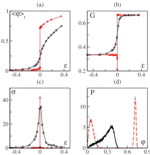
for vectorial noise, and the Binder cumulant exibits a mini-mum at the transition point, indicating a discontinuous phase transition关Figs.1共a兲and1共b兲兴. Simultaneously, the variance is almost␦ peaked. The difference between the two cases is also recorded in the probability distribution function 共PDF兲 of ␸ which is bimodal 共phase coexistence兲 in the vectorial noise case关Figs.1共c兲and1共d兲兴.

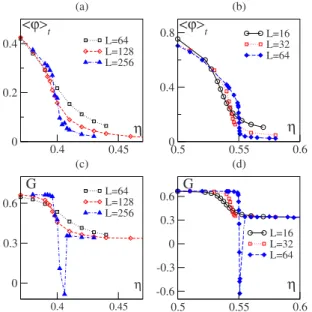
The qualitative difference observed upon changing the way noise is implemented in the dynamics is, however, only a finite-size effect. As shown in 关38兴, the transition in the angular noise case reveals its asymptotic discontinuous char-acter provided large enough system sizes L are considered 关Figs. 2共a兲 and 2共b兲兴. Remaining for now at a qualitative level, we show in Fig.2共c兲a typical time series of the order parameter for the angular noise case in a large system in the transition region. The sudden jumps from the disordered phase to the ordered one and vice versa are evidence for metastability and phase coexistence.

Note that the system size beyond which the transition re-veals its discontinuous character for the angular noise case at

-0.4 0 0.4 ε 0 0.5 1 _<ϕ> t (a) -0.4 0 0.4 ε 0.2 0.4 0.6 G (b) -0.4 0 0.4 ε 0 20 40 σ (c) 0 0.3 0.6 0.9 ϕ 0 5 10 P (d)

FIG. 1. 共Color online兲 Typical behavior across the onset of col-lective motion for moderate-sized models 共␳=2, v0= 0.5, L = 64兲

with angular共black circles兲 and vectorial noise 共red triangles兲. The reduced noise amplitude ␧ = 1 −␩/␩tis shown on the abscissa

共tran-sition points estimated at␩_t= 0.6144共2兲—vectorial noise—and ␩_t = 0.478共5兲—angular noise兲. 共a兲 Time-averaged order parameter 具␸共t兲典t.共b兲 Binder cumulant G. 共c兲 Variance ␴ of ␸. 共d兲 Order

pa-rameter distribution function P at the transition point. Bimodal dis-tribution for vectorial noise dynamics共red dashed line兲; unimodal shape for angular noise共black solid line兲. Time averages have been computed over 3 ⫻ 105_{time steps.}

0.45 0.5 0.55 η 0 0.2 0.4 <ϕ>t L=64 L=128 L=256 (a) 0.45 0.5 0.55 η -0.6 -0.3 0 0.3 0.6 G L=64 L=128 L=256 (b) 0 _2×105 4×105 6×105 8×105 t 0 0.1 0.2 0.3 ϕ (c)

FIG. 2. 共Color online兲 FSS analysis of angular noise dynamics 共␳=2, v0= 0.5, time averages computed over 2 ⫻ 107 time steps兲.

Time-averaged order parameter共a兲 and Binder cumulant 共b兲 as a function of noise for various system sizes L.共c兲 Piece of an order parameter time series close to the transition point 共L=256, ␩ = 0.476兲.

density ␳= 2 and velocity v0= 0.5—the conditions of the original papers by Vicsek et al.—is of the order of L = 128, the maximum size then considered. It is clear also from Fig. 1that the discontinuous nature of the transition appears ear-lier, when the system size is increased, for vectorial noise than for angular noise. Thus, finite-size effects are stronger for angular noise. The same is true when one is in the pres-ence of repulsive interactions共Fig.3兲. Finally, the same sce-nario holds in three space dimensions, with a discontinuous phase transition separating the ordered from the disordered phases for both angular and vectorial noise共Fig.4兲.

Before proceeding to a study of the complete phase dia-gram, we detail now how a comprehensive FSS study can be performed on a particular case.

B. Complete FSS analysis

For historical reasons, the following study has been per-formed on the model with vectorial noise and repulsive force 关Eq. 共6兲兴. It has not been repeated in the simpler case of the “pure” Vicsek model because its already high numerical cost would have been prohibitive due to the strong finite-size ef-fects.

As a first step, we estimated the correlation time ␶共L兲, whose knowledge is needed to control the quality of time averaging: the duration T of numerical simulations has been taken much larger than␶共L兲 共T=100␶in the largest systems, but typically 10 000␶for smaller sizes兲. Moreover,␶is also useful to correctly estimate the statistical errors on the vari-ous moments 共as 具␸典t, ␴, and G兲 of the PDF of the order

parameter, for which we used the jackknife procedure关47兴. The correlation time was estimated near the transition共where it is expected to be largest兲 as function of system size L

measuring the exponential decay rate of the correlation func-tion关Fig.5共a兲兴

C共t兲 = 具␸共t0兲␸共t0+ t兲典t−具␸共t0兲典t₀

2

⬃ exp

冉

␶

冊

We found␶to vary roughly linearly with L关see Fig.5共b兲兴. It is interesting to observe that, at equilibrium, one would ex-pect␶to scale as关48兴

␶= Ld/2exp共␬Ld−1兲,

where␬is the surface tension of the metastable state. There-fore, our result implies a very small or vanishing surface tension ␬Ⰶ 1 / L, a situation reminiscent of observations made in the cohesive case关22兴, where the surface tension of a cohesive droplet was found to vanish near the onset.

0.4 0.45 η 0 0.2 0.4 <ϕ>_t L=64 L=128 L=256 (a) 0.4 0.45 η 0 0.3 0.6 G _L=64 L=128 L=256 (c) 0.5 0.55 0.6 η 0 0.4 0.8<ϕ>t _L=16 L=32 L=64 (b) 0.5 0.55 0.6 η -0.6 -0.3 0 0.3 0.6 G L=16 L=32 L=64 (d)

FIG. 3. 共Color online兲 Transition to collective motion with short-range repulsive interactions. Left panels: angular noise. Right panels: vectorial noise.共a兲,共b兲 Order parameter vs noise amplitude at different system sizes.共c兲,共d兲 Binder cumulant G as a function of noise amplitude.共␳=2, v0= 0.3, time averages carried over 107time

steps.兲 0.3 0.4 η 0 0.2 0.4 <ϕ>_t L = 96 L = 128 (a) 0.3 0.4 η -0.6 0 0.6 G L = 96 L = 128 (c) 0.4 0.6 0.8 η 0 0.4 0.8 <ϕ>_t L = 16 L = 32 (b) 0.4 0.6 0.8 η 0 0.3 0.6 G L = 16 L = 32 (d)

FIG. 4. 共Color online兲 Transition to collective motion in three spatial dimensions. Left panels: angular noise. Right panels: vecto-rial noise.共a兲,共b兲 Time-averaged order parameter vs noise amplitude at different system sizes.共c兲,共d兲 Binder cumulant G as a function of noise amplitude.共␳=0.5, v0= 0.5, time averages carried over 105

time steps.兲 0 100 200 300 t 0 0.4 0.8 C (a) 0 64 128 L 20 30 40 50 τ (b) 0 100 200 t -4 -2 0 _ln(C)

FIG. 5. Correlation time ␶ of the order parameter near the tran-sition point for vectorial noise dynamics with repulsion. System parameters are ␳ = 2, v₀= 0.5, and␩⬇␩_t.共a兲 Time correlation func-tion C共t兲 at L=128. The lin-log inset shows the exponential decay. 共b兲 Correlation time ␶ as a function of system size L. The dashed line marks linear growth with L. Correlation functions were com-puted on samples of⬇106_{realizations for typically 10}3_{time steps.}

Following Borgs and Kotecky关49兴, the asymptotic coex-istence point␩t共i.e., the first-order transition point兲 can be

determined from the asymptotic convergence of various mo-ments of the order parameter PDF. First, the observed dis-continuity in 具␸共t兲典t, located at ␩␸共L兲, is expected to con-verge exponentially to␩twith L. Second, the location of the

susceptibility peak␩␴共L兲—which is the same as the peak in

␴ provided some fluctuation-dissipation relation holds 共see the Appendix兲—also converges to ␩t, albeit algebraically

with an exponent␥_␴. Third, the location of the minimum of

G, ␩G共L兲, is also expected to converge algebraically to ␩t

with an exponent␥G=␥␴.

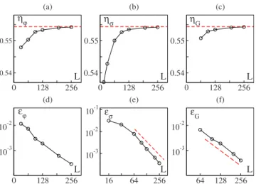
Interestingly, the value taken by these exponents actually depends on the number of phases and of the dimension d of the system: for two-phase coexistence one has␥G=␥␴= 2d, while for more than two phases ␥_G=␥_␴= d. In Fig. 6, we show that our data are in good agreement with all these pre-dictions. The three estimates of␩t are consistent with each

other within numerical accuracy. Moreover, ␩␸共L兲 is found to converge exponentially to the transitional noise amplitude, while both ␩␴共L兲 and ␩G共L兲 show algebraic convergence

with an exponent close to 2. This agrees with the fact that, due to the continuous rotational symmetry, the ordered phase is degenerate and amounts to an infinite number of possible phases.

C. Hysteresis

One of the classical hallmarks of discontinuous phase transitions is the presence, near the transition, of the

hyster-esis phenomenon: on ramping the control parameter at a fixed共slow兲 rate up and down through the transition point, a hysteresis loop is formed, inside which phase coexistence is manifest 关see Fig. 7共a兲 for the d = 3 case with vectorial noise兴. The size of such hysteresis loops varies with the ramping rate. An intrinsic way of assessing phase coexist-ence and hysteresis is to study systematically the nucleation time ␶↑ needed to jump from the disordered phase to the ordered one, as well as␶↓, the decay time after which the ordered phase falls into the disordered one. Figure 7共b兲 shows, in three space dimensions, how these nucleation and decay rates vary with␩at two different sizes. A sharp diver-gence is observed, corresponding to the transition point. At a given time value␶, one can read, from the distance between the “up” and the “down” curves, the average size of hyster-esis loops for ramping rates of the order of 1 /␶.

D. Phase diagram

The above detailed FSS study would be very tedious to realize when the main parameters ␩, ␳, and v0 are varied systematically, as well as the nature of the noise and the presence or not of repulsive interactions. From now on, to characterize the discontinuous nature of the transition, we rely mainly on the presence, at large enough system sizes L, of a minimum in the variation of the Binder cumulant G with

␩共all other parameters being fixed兲. We call Lⴱ_{the crossover} size marking the emergence of a minimum of G共␩兲.

We are now in the position to sketch the phase diagram in the共␩,␳,v0兲 parameter space. The numerical protocol used is, at given parameter values, to run a large enough system so that the discontinuous character of the transition is seen共i.e.,

L⬎ Lⴱ_{兲. For larger sizes, the location of the transition point} typically varies very little, so that, for most practical pur-poses, locating the 共asymptotic兲 transition point from sys-tems sizes around Lⴱ _{is satisfactory.}

The results presented below are in agreement with simple mean-field-like arguments in the diluted limit: in the small-␳

regime, one typically expects that the lower the density, the

0 128 256 L 10-3 10-2 ε_ϕ (d) 0 128 256 L 0.54 0.55 η_ϕ (a) 16 64 256 L 10-3 10-2 10-1 ε_σ (e) 0 128 256 L 0.54 0.55 η_σ (b) 64 128 256 L 10-3 10-2 ε_G (f) 0 128 256 L 0.54 0.55 η_G (c)

FIG. 6.共Color online兲 FSS analysis of vectorial dynamics with short-range repulsive force 共␳=2, v0= 0.3兲. Convergence of the

finite-size transition points measured from different moments of the order parameter FSS to the asymptotic transition point␩_t共see Fig.

3兲. Upper panels: finite-size transition points estimated from 共a兲 time average,共b兲 variance, and 共c兲 Binder cumulant. The horizontal dashed line marks the estimated asymptotic threshold ␩_t = 0.5544共1兲. Lower panels: scaling of the finite-size reduced noise ␧ = 1 −␩/␩_t transition point. 共d兲 Exponential convergence for the jump location in the time-averaged order parameter.共e兲 Power-law behavior of the variance peak position.共f兲 Power-law behavior of the Binder cumulant minimum. The dashed lines in共e兲 and 共f兲 mark the estimated exponents␥␴= ␥G= 2.

0.6 0.62 0.64 η 0 0.2 0.4 0.6 ϕ (a) 0.55 0.6 0.65 η 102 103 104 τ_↑, τ_↓ L=24 L=32 (b)

FIG. 7. 共Color online兲 Hysteresis in three spatial dimensions with vectorial noise.共a兲 Order parameter vs noise strength along the hysteresis loop observed with a ramp rate of 2 ⫻ 10−6_{per time step}

共␳=1/2, v0= 0.5, L = 32兲. Empty circles mark the path along the

adiabatic increase of noise amplitude; full triangles for adiabatic decrease. 共b兲 Nucleation times from the disordered phase to the ordered phase共␶↑, left curves兲 and vice versa 共␶↓, right curves兲 for

two system sizes关other parameters as in 共a兲兴. Each point is aver-aged over 1000 realizations.

lower the transitional noise amplitude␩t. Indeed, for ⌬tv0of the order of or not much smaller than the interaction range r0 and in the low-density limit␳Ⰶ 1 / r0d, the system can be seen as a dilute gas in which particles interact by short-range or-dering forces only. In this regime, the persistence length of an isolated particle共i.e., the distance traveled before its ve-locity loses correlation with its initial direction of motion兲 varies as v0/␩. To allow for an ordered state, the noise am-plitude should be small enough so that the persistence length remains larger than the average interparticle distance, i.e., 1 /␳1/d

. Thus the transition noise amplitude is expected to behave as

␩t⬃ v0␳1/d. 共10兲 In 关5兴, it was indeed found that ␩t⬃␳␣ with ␣⯝

1 2 in two dimensions. Our own data关Figs.8共a兲–8共c兲兴 now confirm Eq. 共10兲 for both the angular and vectorial noise in two and three spatial dimensions, down to very small ␳ values. The data deviate from the square-root behavior as the average inter-particle distance becomes of the order of or smaller than the interaction range.

Finally, we also investigated the transition line when v0is varied关Fig.8共d兲兴. For the vectorial noise case, at fixed den-sity, the threshold noise value ␩t is almost constant 共data

obtained at ␳=1₂, not shown兲. For the angular noise, in the small-v0limit where the above mean-field argument does not

apply, we confirm the first-order character of the phase tran-sition down to v0⬇0.05 for both angular and vectorial noise 关Figs. 9共b兲 and 9共d兲兴. For even smaller values of v0, the investigation becomes numerically too costly 共see the next subsection兲. Note that␩tseems to be finite when v0→ 0+, a limit corresponding to the XY model on a randomly con-nected graph. Still, for angular noise, the large-velocity limit is also difficult to study numerically. Again, we observe that the transition is discontinuous as far as we can probe it, i.e.,

v₀= 20关Figs.9共a兲and9共b兲兴.

E. Special limits and strength of finite-size effects We now discuss particular limits of the models above to-gether with the relative importance of finite-size effects. Re-call that these are quantified by the estimated value of the crossover size Lⴱ _{beyond which the transition appears} dis-continuous. All the following results have been obtained for

d= 2. Partial results in three dimensions indicate that the same conclusions should hold there. Keep in mind that in all cases reported the transition is discontinuous. We are just interested here in how large a system one should use in order to reach the asymptotic regime.

Figure10共a兲shows that finite-size effects are stronger for angular noise than for vectorial noise for all densities ␳ at which we are able to perform these measurements. Note in particular that, at␳= 2, the density originally used by Vicsek

et al., Lⴱ_{⬃128 for angular noise, while it is very small for} vectorial noise, confirming the observation made in Sec. III A.

In the small-␳ limit, the discontinuous character of the transition appears later and later, with Lⴱ _{roughly diverging}

0 1 2 3 ρ 0 0.2 0.4 0.6 ηt (b) 0 0.2 0.4 v₀ 0 0.2 0.4 η_t (d) 0.01 1 ln(ρ) 0.2 1_ln(η t) 0.01 1 ρ 0.04 0.2 η_t 0 2 4 ρ 0 0.2 0.4 η_t (a) 0 1 2 ρ 0 0.4 0.8 η_t (c) 0.01 1 ρ 0.25 0.5 η_t

FIG. 8.共Color online兲 Asymptotic phase diagrams for the tran-sition to collective motion. 共a兲 Two space dimensions: threshold amplitude ␩t for angular noise as a function of density ␳ at v0

= 0.5. Inset: Log-log plot to compare the low-density behavior with the mean-field predicted behavior␩t⬃

冑

in共a兲, but with vectorial noise dynamics. 共c兲 Noise-density phase diagram in three dimensions for vectorial noise dynamics at fixed velocity v₀= 0.5. In the log-log inset the transition line can be com-pared with the predicted behavior␩t⬃␳1/3共dashed red line兲. 共d兲

Two space dimensions: threshold amplitude␩_tfor angular noise as a function of particle velocity v0 at fixed density ␳ = 1 / 2 共black

circles兲 and 1/8 共red triangles兲. The horizontal dashed line marks the noise amplitude considered in Ref.关39兴 共see Sec. III F兲.

0.64 0.65 0.66 0.67 η 0 0.1 0.2 〈ϕ〉t v0=5, L=200 v0=10, L=250 v0=20, L=300 (a) 0.64 0.65 0.66 0.67 η -0.5 0 0.5 G (c) 0.15 0.2 0.25 η 0 0.2 0.4 0.6 〈ϕ〉t (b) 0.15 0.2 0.25 η 0.2 0.4 0.6 G L=1024 L=256 (d)

FIG. 9. 共Color online兲 First-order transition for angular noise dynamics at high共left panels兲 and low 共right panels兲 velocity v0.

Typical averaging time is⬇106_{time steps.共a兲 Time-averaged order}

parameter and 共c兲 Binder cumulant at large particle velocity for angular noise in two spatial dimensions at increasing velocities and Lⲏ Lⴱ_{共␳=2兲. 共b兲 Time-averaged order parameter and 共d兲 Binder}

as 1 /

冑

The large-␳limit reveals a difference between angular and vectorial noise: while Lⴱ_{remains small for vectorial noise, it} seems to diverge for angular noise关Fig.10共a兲兴, making this case difficult to study numerically.

We also explored the role of the microscopic velocity v0 in the strength of finite-size effects. Qualitatively, the effects observed are similar to those just reported when the density is varied 关Fig. 10共b兲兴. In the small-v0 limit, we record a strong increase of Lⴱ_{as v}

0→ 0 for both types of noise. In the large-velocity limit, Lⴱ_{decreases for vectorial noise, whereas} it increases for angular noise.

F. Summary and discussion

The summary of the above lengthy study of the order-disorder transition in Vicsek-like models is simple: for any finite density␳, any finite velocity v0, and both types of noise introduced, the transition is discontinuous. This was ob-served even in the numerically difficult limits of large or small ␳ or v0. These results contradict recent claims made about the angular noise case 共original Vicsek model兲. We now comment on these claims.

Vicsek and co-workers 关39兴 showed that, when the den-sity and the noise intenden-sity are kept fixed, a qualitative change is observed when v0is decreased: for not too small v0 values, in the ordered phase, particles diffuse anisotropically 共and the transition is discontinuous兲, while diffusion be-comes isotropic at small v0, something interpreted as a sign of a continuous transition in this region. Rather than the con-voluted arguments presented there, what happens is in fact rather simple: by decreasing v0 at fixed␳ and␩, one can in fact cross the transition line, passing from the ordered phase 共where particles obviously diffuse anisotropically due to the transverse superdiffusive effects discussed in Sec. IV C兲 to the disordered phase. Our Fig. 8共d兲, obtained in the same conditions as in 关39兴 共apart from harmless change of the time-updating rule兲, shows that if one keeps ␩= 0.1 共as in 关39兴兲, one crosses the transition line at about v0⯝0.1, the

value invoked by Vicsek and co-workers to mark a crossover from discontinuous to “continuous” transitions.

In a recent Letter关40兴, Aldana et al. study order-disorder phase transitions in random network models and show that the nature of these transitions may change with the way noise is implemented in the dynamics共they consider the an-gular and vectorial noises defined here兲. Arguing that these networks are limiting cases of Vicsek-like models, they claim that the conclusions reached for the networks carry over to the transition to collective motion of the Vicsek-model-like systems. They conclude in particular that in the case of “angular” noise the transition to collective motion is continuous. We agree with the analysis of the network mod-els, but the claim that they are relevant as limits of Vicsek-like models is just wrong: the data presented there共Fig. 1 of 关40兴兲 to substantiate this claim are contradicted by our Figs. 9共a兲and9共c兲共see also 关50兴兲 obtained at larger system sizes. Again, for large enough system sizes, the transition is indeed discontinuous. Thus, at best, the network models of Aldana

et al.constitute a singular v0→ ⬁ limit of Vicsek-like mod-els.

IV. NATURE OF THE ORDERED PHASE

We now turn our attention to the ordered, symmetry-broken phase. In previous analytical studies, it has often been assumed that the density in the ordered phase is spatially homogeneous, albeit with possibly large fluctuations 共see, e.g., 关8兴兲. This is indeed what has been reported in early numerical studies, in particular by Vicsek et al. 关9兴. In the following, we show that this is not true in large enough sys-tems, where, for a wide range of noise amplitudes near the transition point, density fluctuations lead to the formation of localized, traveling, high-density, and high-order structures. At low enough noise strength, though, a spatially homoge-neous ordered phase is found, albeit with unusually strong density fluctuations.

A. Traveling in bands

Numerical simulations of the ordered phase dynamics 共␩⬍␩t兲, performed at large enough noise amplitudes, are

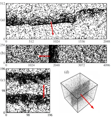
characterized by the emergence of high-density moving bands共d=2兲 or sheets 共d=3兲. Typical examples are given in Figs. 11 and 12. These moving structures appear for large enough systems after some transient. They extend transver-sally with respect to the mean direction of motion, and have a center of mass velocity close to v0. While particles inside bands are ordered and, in the asymptotic regime, move co-herently with the global mean velocity, particles lying out-side bands—in low-density regions—are not ordered and perform random walks.

As shown in Fig. 11共a兲–11共c兲 for the angular noise dy-namics共1兲, there exists a typical system size Lb, below which

the bands or sheets cannot be observed. Numerical simula-tions indicate that Lbdepends only weakly on the noise

am-plitude and is of the same order of magnitude as the cross-over size marking the appearance of the discontinuous character of the transition: Lb⬇Lⴱ. It is therefore numerically

0.01 0.1 1 ρ 101 102 103L * 0.1 1 10 v₀ 10 100 1000 L * (b) 0 2 4 ρ 0 300 600 L* (a)

FIG. 10.共Color online兲 Crossover system size Lⴱ_{above which}

the discontinuous character of the transition appears关as testified by the existence of a minimum in the G共␩兲 curve兴. Black circles: an-gular noise. Red triangles: vectorial noise.共a兲 Lⴱ_{vs ␳ for v}

0= 0.5.

Inset: the low-density behavior in log-log scales; the dashed line marks a power-law divergence proportional to 1 /

冑

0at

easier to observe bands in the ordered phase of vectorial noise dynamics共3兲, as in Fig.11共d兲.

Bands may be observed asymptotically without and with a repulsive interaction关Fig.12共c兲兴 and for both kinds of noise. They appear for various choices of boundary conditions关see, for instance, Figs.12共a兲and12共b兲, where reflecting bound-ary conditions have been employed兴, which may play a role in determining the symmetry-broken mean direction of mo-tion. For instance, bands traveling parallel to one of the axes are favored when periodic boundary conditions are employed in a rectangular box 共they represent the simplest way in which an extended structure can wrap around a torus, and are thus reached more easily from disordered initial conditions兲, but bands traveling in other directions may also appear, al-beit with a smaller probability.

Bands can be described quantitatively through local quan-tities, such as the local density ␳ᐉ共xជ, t兲, measured inside a domain V共xជ兲 centered around xជ, and the local order param-eter

␸ᐉ共xជ,t兲 = 1

v₀兩具vជi共t兲典rជi僆V共xជ兲兩. 共11兲

Further averaging these local quantities perpendicularly to the mean velocity 共7兲, one has the density profile ␳_⬜共x储, t兲

=具␳ᐉ共xជ, t兲典_⬜ and the order parameter profile ␸_⬜共x储, t兲

=具␸ᐉ共xជ, t兲典_⬜, where x储 indicates the longitudinal direction

with respect to the mean velocity. Bands are characterized by a sharp kink in both the density and the order parameter profiles关see Figs.13共a兲,13共c兲, and13共d兲兴. They are typically

asymmetric, as can be expected for moving structures, with a rather sharp front edge, a well-defined mid-height width

w—which typically is of the same order as Lb—and an

ex-ponentially decaying tail with a characteristic decay length of the order of w关Fig.13共b兲兴.

Large systems may accommodate several bands at the same time, typically all moving in the same direction关see, for instance, Fig.11共c兲and the density profile in Fig.14共e兲兴. However, they do not form well-defined wave trains, but rather a collection of solitary objects, as hinted by the fol-lowing numerical experiments.

We investigated the instability of the density-homogeneous, ordered state in a series of numerical simula-tions starting from particles uniformly distributed in space but strictly oriented along the major axis in a large rectangu-lar domain. Figures14共a兲and14共b兲show space-time plots of the density profile: initially flat, it develops structures with no well-defined wavelength关Fig.14共c兲兴. Density fluctuations destroy the initially ordered state in a rather unusual way: a dynamical Fourier analysis of the density profile show a weakly peaked, wide band of wavelengths growing

subexpo-nentially 关Fig. 14共d兲兴. This is at odds with a finite-wavelength supercritical instability, which would lead to a wave train of traveling bands. Furthermore, the asymptotic

0 32 64 0 32 64 (a) 0 512 1024 0 512 1024 (c) 0 128 256 0 128 256 (b) 0 32 64 0 32 64 (d)

FIG. 11.共Color online兲 Typical snapshots in the ordered phase. Points represent the position of individual particles and the red ar-row points along the global direction of motion. 共a兲–共c兲 Angular noise, ␳ = 1 / 2, v0= 0.5,␩= 0.3, and increasing system sizes,

respec-tively, L = 64, 256, and 1024. Sharp bands can be observed only if L is larger than the typical bandwidth w.共d兲 Vectorial noise, ␳=1/2, v₀= 0.5,␩= 0.55, and L = 64: bands appear at relatively small system sizes for this type of noise. For clarity, only a representative sample of 10 000 particles is shown in共b兲 and 共c兲. Boundary conditions are periodic. 0 512 1024 1536 2048 0 512 0 1024 2048 3072 4096 0 256 0 98 196 0 98 196 0 98 196 0 98 196 (c) (b) (a) (d)

FIG. 12. 共Color online兲 Same as Fig.11but in different geom-etries and boundary conditions or space dimensions.共a兲,共b兲 Vecto-rial noise共␩= 0.325, ␳ = 1 / 8, and v0= 0.5兲; boundary conditions are

periodic along the y 共vertical兲 axis and reflecting in x. 共a兲 A long single band travels along the periodic direction.共b兲 The domain size along the periodic direction is too small to accommodate bands, and a single band bouncing back and forth along the nonperiodic direc-tion is observed.共c兲 Angular noise, repulsive force, and periodic boundary conditions共␳=2,␩= 0.23, and v0= 0.3兲. 共d兲 High-density

sheet traveling in a three-dimensional box with periodic boundary conditions 共angular noise with amplitude ␩= 0.355, ␳ = 1 / 2, and v₀= 0.5兲.

共late-time兲 power spectra of the density profiles are not peaked around a single frequency either, but rather broadly distributed over a large range of wave numbers关Fig.14共f兲兴. In the asymptotic regime, bands are extremely long-lived metastable 共or possibly stable兲 objects, which are never equally spaced关a typical late-time configuration is shown in Fig.14共e兲兴.

To summarize, the emerging band or sheet structure in the asymptotic regime is not a regular wave train characterized by a single wavelength, but rather a collection of irregularly spaced localized traveling objects, probably weakly interact-ing through their exponentially decayinteract-ing tails.

B. Low-noise regime and giant density fluctuations As the noise amplitude is decreased away from the tran-sition point, bands are less sharp, and eventually disappear, giving way to an ordered state characterized by a homoge-neous local order parameter and large fluctuations of the lo-cal density.

A quantitative measure of the presence, in the ordered phase, of structures spanning the dimension transverse to the mean motion共i.e., bands or sheets兲 is provided by the vari-ances of the density and order parameter profiles:

⌬␳_⬜2共t兲 = Š关␳_⬜共x储,t兲 − 具␳_⬜共x储,t兲典储兴2‹储,

⌬␸_⬜2共t兲 = Š关␸_⬜共x储,t兲 − 具␸_⬜共x储,t兲典储兴2‹储, 共12兲

where具·典储indicates the average of the profile in the

longitu-dinal direction with respect to mean velocity. Indeed, these

profile widths vanish in the infinite-size limit except if band or sheet structures are present.

In Figs.15共a兲and15共b兲, we plot these profile widths av-eraged over time as a function of noise amplitude. Both quantities present a maximum close to the transition point in the ordered phase, and drop drastically as soon as the disor-dered phase is entered. Lowering the noise away from the transition point, these profiles decrease steadily: bands and

0 x_// 256 0 3 6 ρ_⊥ 0 0.4 0.8 ϕ_⊥ 40 60 80 x_// 0.2 1 ρ_⊥ (b) 0 48 96 0 48 96 (c) 0 x_// 96 0 1 2 3 _ρ ⊥ (d) 0 0.4 0.8 ϕ_⊥ (a)

FIG. 13.共Color online兲 共a兲 Typical density 共black line兲 and or-der parameter共dashed red line兲 profiles for bands in two dimensions 共vectorial noise, ␳=2,␩= 0.6, and v0= 0.5兲. 共b兲 Tail of the density

profile shown in共d兲 共black line兲 and its fit 共blue dashed line兲 by the formula ␳_⬜共x储, t兲⬇a0+ a1共t兲exp共−x储/w兲, with w⬇6.3 共lin-log

scale兲. 共c兲,共d兲 Traveling sheet in three dimensions 共angular noise, ␳ = 1 / 2,␩= 0.355, and v0= 0.5兲. 共c兲 Projection of particle positions

on a plane containing the global direction of motion共marked by red arrow兲. 共d兲 Density 共black line兲 and order parameter 共dashed red line兲 profiles along the direction of motion x储.

0 100 200 k 0 0.4 0.8 S (c) 0 400 800 t 0 0.4 0.8 S k (d) 0 800 1600 x_// 0 4 8 ρ_⊥ (e) 0 100 200 k 0 0.4 0.8 S (f) 0 75 0.05 0.1

FIG. 14. 共Color online兲 Emergence of high-density high-order traveling bands 共d=2兲 from a spatially homogeneous 共uniformly distributed random positions兲 initial condition with all particle ve-locities oriented along the major axis of a 196⫻ 1960 domain with periodic boundary conditions. Vectorial noise of amplitude␩= 0.6, density ␳ = 2, and v₀= 0.5.共a兲 Space-time plot of the density profile. Time is running from left to right from t = 0 to 12 000, while the longitudinal direction is represented on the ordinates. Color scale from blue共low values兲 to red 共high values兲. 共b兲 Same as 共a兲 but at later times共from t=148 000 to 160 000兲. 共c兲 Spatial Fourier power spectrum S of an early density profile共t=12 000兲. 共d兲 Early-time evolution of selected Fourier modes k = 10, 23, 28, 33, 41, 76, and 121共the black lowest curve is for k=10, the other curves are not significantly different兲. Inset: average over 50 different runs. 共e兲 Density profile at a late time关t=160 000, final configuration of 共b兲兴. 共f兲 Same as 共c兲 but for the late-time density profile of 共e兲.

sheets stand less sharply out of the disordered background 关Fig.15共c兲兴. At some point 关␩⬇0.3 for the parameter values considered in Figs. 15共a兲and 15共b兲兴, bands rather abruptly disappear and are no longer well-defined transversal objects. It is difficult to define this point accurately, but it is clear that for lower noise intensities the local order parameter is strongly homogeneous in space. Nevertheless, fluctuations in the density field are strong 关Fig. 15共d兲兴, but can no longer give rise to共meta兲stable long-lived transverse structures.

Density fluctuations in the bandless regime are in fact anomalously strong: measuring number fluctuations in sub-systems of linear size ᐉ, we find that their root mean square ⌬n does not scale like the square root of n =␳ᐉd_{, the mean}

number of particles they contain; rather we find ␴共n兲⬀n␣ with␣⬇0.8 both in d=2 and in d=3 关Fig. 16共a兲兴. This is reminiscent of the recent discovery of “giant density fluctua-tions” in active nematics关14,51,52兴. However, the theoretical argument which initially predicted such fluctuations 关53兴 cannot be invoked directly in the present case. 共Indeed, the above value of␣, although needing to be refined, does not seem to be compatible with the prediction␣=1₂+_d1 made in 关53兴.兲 More work is needed to fully understand under what circumstances the coupling between density and order in sys-tems of “active” self-propelled particles gives rise to such anomalous density fluctuations.

C. Transverse superdiffusion

According to the predictions of Toner and Tu关8,33,34兴, the dynamics of the symmetry-broken ordered phase of polar

active particles should be characterized by a superdiffusive mean square displacement

⌬x_⬜=

冑

in the direction共s兲 transversal to the mean velocity. In par-ticular, in d = 2 one has关34兴

⌬x_⬜2 ⬃ t␯ _共14兲

with␯= 4 / 3. While this analytical result has been success-fully tested by numerical simulations of models with cohe-sive interactions 关34,38兴, numerical simulations in models without cohesion present substantial difficulties, mainly due to the presence of continuously merging and splitting sub-clusters of particles moving coherently共as discussed in Sec. IV D兲. As a consequence, an ensemble of test particles in a cohesionless model is exposed to different “transport” re-gimes共with respect to center of mass motion兲 which are not well separated in time. When the mean displacement is av-eraged at fixed time, this tends to mask the transverse super-diffusion.

To overcome this problem, we chose to follow关54兴 and to measure␶2, the average time taken by two particles to double their transverse separation distance ␦_⬜. From Eq. 共14兲 one immediately has

␶2⬃␦⬜ 2/␯

共15兲 with 2 /␯= 3 / 2 in d = 2. In order to easily separate the trans-verse from the parallel component, we considered an ordered system in a large rectangular domain with periodic boundary conditions and the mean velocity initially oriented along the long side. The mean direction of motion then stays oriented along this major axis, so that we can identify the transverse direction with the minor axis. Furthermore, a high density and a small共angular兲 noise amplitude 共corresponding to the

0.2 0.4 η 0 0.8 1.6 <∆ρ_⊥>t (a) 0.2 0.4 η 0 0.1 0.2 <∆ϕ_⊥>t (b) 0 2 4 6 ρ_⊥ (c) x // 0 2 4 6 ρ_⊥ (d) 0 10240 0.5 1 ϕ_⊥ 0 x_// 10240 0.5 1 ϕ_⊥

FIG. 15.共Color online兲 共a兲,共b兲 Time-averaged profile width for both density 共a兲 and order parameter 共b兲 as a function of noise amplitude in the ordered phase共angular noise, 1024⫻256 domain, global motion along the major axis, ␳ = 2, and v0= 0.5兲. The dashed

vertical blue line marks the order-disorder transition.共c兲,共d兲 Typical instantaneous profiles along the long dimension of the system de-scribed in共a兲 and 共b兲 for intermediate noise value 关共b兲␩= 0.4兴 and in the bandless regime关共c兲␩= 0.15兴.

100 101 102 δ, δ ⊥ 102 104 106 _τ 2 (b) 102 104 <n> 102 104 ∆n (a)

FIG. 16.共Color online兲 Giant density fluctuation and transverse superdiffusion in the bandless ordered phase.共a兲 Anomalous density fluctuations共see text兲: ⌬n scales approximately like n0.8_{共the dashed}

line has slope 0.8兲 both in two dimensions 共black circles, L=256, ␳ = 2, v0= 0.5, angular noise amplitude␩= 0.25兲 and in three

dimen-sions共red triangles, L=64, ␳=1/2 v0= 0.5, vectorial noise

ampli-tude␩= 0.1, values shifted for clarity兲. 共b兲 Average doubling time ␶2

of the transverse共with respect to mean velocity兲 interparticle dis-tance ␦_⬜. Black circles: ordered bandless regime 共␳=4, angular noise amplitude ␩= 0.2 in a rectangular box of size 1024⫻ 256兲. The black dashed line marks the expected growth ␶2⬃␦_⬜3/2. Red

squares: same but deep in the disordered phase共␳=4, angular noise amplitude ␩= 1, L = 512兲. The dot-dashed red line shows normal diffusive behavior: ␶2⬃␦2.

bandless regime兲 have been chosen to avoid the appearance of large, locally disordered patches.

Our results关Fig. 16共b兲兴 confirm the prediction of Toner and Tu: transverse superdiffusion holds at low enough noise, while normal diffusion is observed in the disordered, high-noise phase. Note that the systematic deviation appearing in our data at some large scale is induced by large fluctuations in the orientation of the global mean velocity during our numerical simulations共not shown here兲.

We take the opportunity of this discussion to come back to the superdiffusive behavior of particles observed in the transition region关21兴. There, subclusters emerge and propa-gate ballistically and isotropically due to the absence of a well-established global order. Particle trajectories consist in “ballistic flights,” occurring when a particle is caught in one of these coherently moving clusters, alternated with ordinary diffusion in disordered regions. The mean square displace-ment of particles exhibits the scaling ⌬x2_{=具兩xជ共t兲−xជ共0兲兩}2_典

i

⬀ t5/3_{关21兴. In view of our current understanding of the} dis-continuous nature of the transition, we now tend to believe that this isotropic superdiffusion is probably not asymptotic.

D. Internal structure of the ordered region

We now turn our attention to the internal structure of the ordered regimes. As we noted in the previous section, these regimes do not consist of a single cluster of interacting par-ticles moving coherently. Even in the case where high-density bands or sheets are present, these are in fact dynami-cal objects made of splitting and merging clusters. Note that, for the models considered here, clusters are unambiguously defined thanks to the strictly finite interaction range r0.

As noticed first by Aldana and Huepe关7兴, clusters of size

n are distributed algebraically in the ordered region, i.e.,

P共n兲⬃n−␮_{. But a closer look reveals that the exponent ␮} characterizing the distribution of cluster sizes changes with the distance to the transition point. For noise intensities not too far from the threshold, when bands are observed, we find

␮ values larger than 2, whereas ␮⬍ 2 in the bandless re-gimes present at low noise intensities关Fig.17共a兲and17共b兲兴. Thus, bands are truly complex, nontrivial structures emerging out of the transverse dynamics of clusters with a well-defined mean size共since␮⬎ 2兲. It is only in the band-less regime that one can speak, as do Aldana and Huepe, of “strong intermittency.” We note in passing that the parameter values they considered correspond in fact to a case where bands are easily observed共at larger sizes than those consid-ered in关7兴兲. Thus, clusters do have a well-defined mean size in their case. Consequently, the probability distribution P共␸兲 of the order parameter␸does not show the behavior reported in Fig. 1 of关7兴 as soon as the system size is large enough. Whether in the band and sheet regime or not, P共␸兲 shows essentially Gaussian tails, is strongly peaked around its mean, and its variance decreases with increasing system size 关Figs.17共c兲and17共d兲兴.

Although the picture of intermittent bursts between “lami-nar” intervals proposed by Aldana and Huepe has thus to be abandoned, the anomalous density fluctuations reported in the previous section are probably tantamount to the strong

intermittency of cluster dynamics in the bandless regime. Again, these phenomena, reported also in the context of ac-tive nematics关14,51,53兴, deserve further investigation.

E. Phase ordering

The ordered regimes presented above are the result of some transient evolution. In particular, the bands and sheets are the typical asymptotic structures appearing in finite do-mains with appropriate boundary conditions. In an infinite system, the phase ordering process is, on the other hand, infinite, and worth studying for its own sake.

Numerically, we have chosen to start from highly disor-dered initial conditions which have a homogeneous density and vanishing local order parameter. In practice, we quench a system “thermalized” at strong noise to a smaller, subcritical,

␩value. Typical snapshots show the emergence of structures whose typical scale seems to increase fast共Fig.18兲. During this domain growth, we monitor the two-point spatial corre-lation function of both the density and velocity fields. These fields are defined by a coarse-graining over a small length scale ᐉ 共typically 4兲. These correlation functions have an unusual shape关Fig.19共a兲兴: after some rather fast initial de-cay, they display an algebraic behavior whose effective ex-ponent decreases with time, and finally display a near-exponential cutoff. As a result, they cannot be easily collapsed on a single curve using a simple, unique, rescaling length scale. Nevertheless, using the late exponential cutoff, a correlation length␰can be extracted. Such a length scale␰

grows roughly linearly with time关Fig.19共b兲兴. Qualitatively

102 104 n 102 104 106 _P(n) (a) 102 104 n 102 104 106 _P(n) (b) 0.94 0.96 0.98 ϕ 102 104 P(ϕ) (c) 0 0.3 0.6 ϕ 102 104 _P(ϕ) (d) slope -1.8 slope -2.3

FIG. 17. 共Color online兲 共a兲,共b兲 Cluster size distributions 共arbi-trary units兲 for domain sizes L=32 共black兲, 128 共cyan兲, and 512 共green兲 from left to right 共d=2, ␳=2, v0= 0.5, angular noise兲. 共c兲,共d兲

Probability distribution functions of the order parameter ␸ 共arbi-trary units兲 for the same parameters and system sizes as in 共a兲 and 共b兲. 共The most peaked distributions are for the largest size L=512.兲 Left panels共a兲,共c兲,␩= 0.1, bandless regime; Right panels 共b兲,共d兲, regime with bands at␩= 0.4.

similar results are obtained whether or not the noise strength is in the range where bands and sheets appear in finite boxes. We note that the above growth law is reminiscent of that of the so-called model H of the classification of Halperin and Hohenberg关55兴. Since this model describes, in principle, the phase separation in a viscous binary fluid, the fast growth observed could thus be linked to the hydrodynamic modes expected in any continuous description of Vicsek-like mod-els关8,56兴.

V. GENERAL DISCUSSION AND OUTLOOK A. Summary of main results

We now summarize our main results before discussing them at a somewhat more general level.

We have provided ample evidence that the onset of col-lective motion in Vicsek-style models is a discontinuous

共first-order兲 phase transition, with all expected hallmarks, in agreement with关38兴. We have made the 共numerical兲 effort of showing this in the limits of small and large velocity and/or density.

We have shown that the ordered phase is divided into two regions: near the transition and down to rather low noise intensities, solitary structures spanning the directions trans-verse to the global collective velocity 共the bands or sheets兲 appear, leading to an inhomogeneous density field. For weaker noise, on the other hand, no such structures appear, but strong, anomalous density fluctuations exist and particles undergoes superdiffusive motion transverse to the mean ve-locity direction.

Finally, we have reported a linear growth共with time兲 of ordered domains when a disordered configuration is quenched in the ordered phase. This fast growth can prob-ably be linked to the expected emergence of long-wavelength hydrodynamic modes in the ordered phase of active polar particles models.

B. Role of bands and sheets

The high-density high-order traveling bands or sheets de-scribed here appear central to our main findings. They seem to be intimately linked to the discontinuous character of the transition which can, to some extent, be considered as the stability limit of these objects. In the range of noise values where they are observed, the anomalous density fluctuations present at lower noise intensities are suppressed.

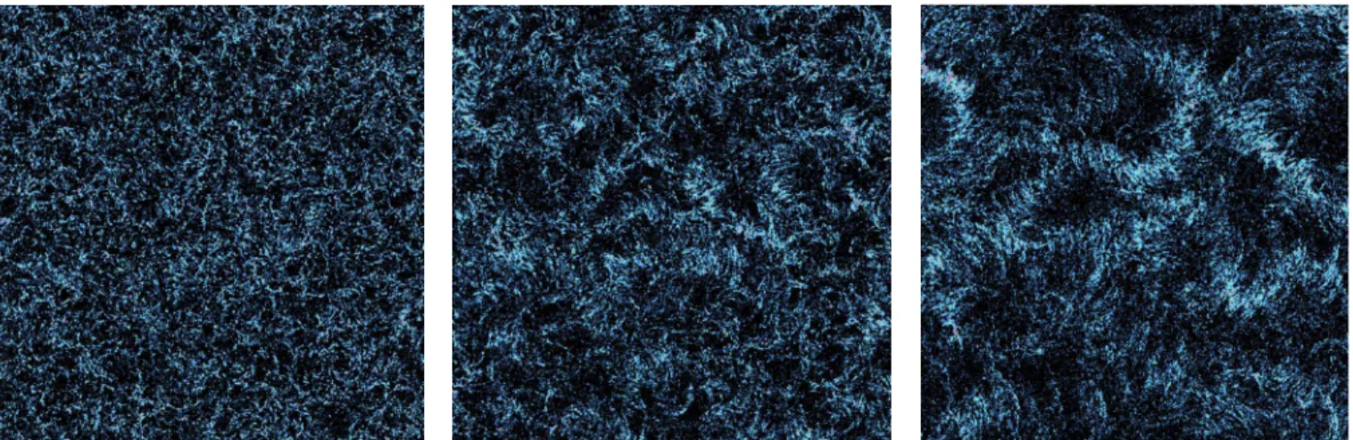
One may then wonder about the universality of these ob-jects. Simple variants of the Vicsek-style models studied here 共e.g., with interactions restricted to binary ones involving only the nearest neighbor兲 do exhibit bands and sheets 关11兴. Moreover, the continuous deterministic description derived by Bertin et al.关11兴 does possess localized, propagating soli-tary solutions rather similar to bands关57兴. Although the sta-bility of these solutions needs to be further investigated, these results indicate that the objects are robust and that their existence is guaranteed beyond microscopic details. How-ever, the emergence of regular, stable, bands and sheets is obviously conditioned to the shape and the boundary condi-FIG. 18.共Color online兲 Phase ordering from disordered initial conditions 共d=2, angular noise amplitude␩= 0.08, ␳ = 1 / 8, v0= 0.5, system

size L = 4096兲. Snapshots of the density field coarse grained on a scale ᐉ=8 at times t=160, 320, and 640 from left to right.

50 100 r 0.3 0.6 C (a) 101 102 103 r 101 102 103 _ξ (b) 10 100 r 10-4 10-2 C

FIG. 19.共Color online兲 Phase ordering as in Fig.18共L=4096, ␳ = 1 / 2, v0= 0.5兲. 共a兲 Two-point density correlation function C共r,t兲

=具␳ᐉ共xជ,t兲␳ᐉ共xជ+rជ,t兲典xជ共coarse grained over a scale ᐉ=4兲 as a

func-tion of distance r =兩rជ兩 at different time steps: from left to right t = 50, 50, 100, 200, 400, 800, and 1600. Noise amplitude is ␩ = 0.25; data have been further averaged over⬇40 different realiza-tions. Inset: log scales reveal the intermediate near-algebraic decay and the quasiexponential cutoff.共b兲 Length scale ␰, estimated from the exponential cutoff positions, as a function of time. Empty black circles:␩= 0.25 as in共a兲 共i.e., regime in which bands are observed asymptotically兲. Red full triangles:␩= 0.1共i.e., in the bandless re-gime兲. The dashed black line marks linear growth.

tions of the domain in which the particles are allowed to move. In rectangular domains with at least one periodic di-rection, these objects can form, span across the whole do-main, and move. But in, say, a circular domain with reflect-ing boundary conditions, they cannot develop freely, bereflect-ing repeatedly frustrated. Nevertheless, simulations performed in such a geometry indicate that the transition remains discon-tinuous, with the ordered phase consisting of one or several dense packets traveling along the circular boundary. Note, though, that these packets intermittently emit elongated structures 共bands兲 traveling toward the interior of the disk before colliding on the boundary. To sum up, bands appear as the “natural” objects in the transition region, but they may be prevented by the boundaries from developing into full-size straight objects.

At any rate, time series of the order parameter such as the one presented in Fig. 2 clearly show that the transition is discontinuous irrespective of the geometry and boundaries of the domain, and thus of whether bands and sheets can de-velop into stable regular structures or not: the sudden, abrupt, jumps from the disordered state to some ordered structure are tantamount to a nucleation phenomenon characteristic of a discontinuous transition.

C. A speculative picture

We would now like to offer the following speculative gen-eral picture. The key feature of the Vicsek-like models stud-ied here—as well as of other models for active media made of self-propelled particles关11,35,56,58,59兴—is the coupling between density and order. Particles are forced to move, and, since they carry information about the order, advection, sity fluctuations, and order are intimately linked. High den-sity means strong local order 共if the noise is low enough兲 because the many particles in a given neighborhood will adopt roughly the same orientation. The reverse is also true: in a highly ordered region, particles will remain together for a long time and thus will sweep many other particles, leading to a denser and denser group.

At a given noise level, one can thus relate, in the spirit of some local equilibrium hypothesis, local density to local or-der. In practice, such an “equation of state” approach can be justified by looking, e.g., at a scatter plot of local order pa-rameter vs local density. Figure 20 reveals that, in the or-dered bandless regime, such a scatter plot is characterized by a plateau over a large range of local density values corre-sponding to order, followed, below some crossover density, by more disordered local patches. The regions in space where local density is below this crossover level do not per-colate in the bandless regime, and order can be maintained very steadily in the whole domain 关this is corroborated by the fact that, in spite of the large, anomalous density fluctua-tions, the order parameter field is, on the other hand, rather constant; see Fig.15共c兲兴. The noise intensity at which bands emerge roughly corresponds to the value where the low-density disordered regions percolate. The remaining discon-nected, dense patches then eventually self-organize into bands or sheets. The emergence of these elongated structures is rather natural: moving packets elongate spontaneously

be-cause they collect many particles; superdiffusion in the di-rections perpendicular to the mean motion endows these na-scent bands and sheets with some “rigidity.” At still stronger noise, the bands and sheets are destroyed and global order disappears.

The above features are at the root of the approach by Toner and Tu关8,33,34兴. Their predictions of strong density fluctuations, transverse superdiffusion, and peculiar sound propagation properties are correct as long as bands or sheets do not exist, i.e., for not too strong noise intensities. This is indeed in agreement with their assumption that the density field is statistically homogeneous in the frame moving at the global velocity共albeit with strong fluctuations兲, which is true only in the bandless regime.

D. Outlook

The results presented here are almost entirely numerical. Although they were obtained with care, they need to be ul-timately backed up by more analytical results. A first step is the derivation of a continuous description in terms of a den-sity and a velocity field共or some combination of the two兲, which would allow one to go beyond microscopic details. In that respect the deterministic equation derived by Bertin et

al. from a Boltzmann description in the dilute limit 关11兴 is encouraging. However, one may suspect that intrinsic fluc-tuations are crucial in the systems considered here if only because some of the effective noise terms will be

multiplica-0 2 4 6 _ρ l 0 0.5 1 1.5 |θlocal -θglobal | (a) 0 2 4 6 _ρ l 0 0.5 1 1.5 |θlocal -θglobal | (b) 0 2 4 6 _ρ l 0 0.5 1 1.5 |θlocal -θglobal | (c) 0 2 4 6 _ρ l 0 0.5 1 1.5 |θlocal -θglobal | (d) η=0.1 η=0.2 η=0.3 η=0.4

FIG. 20.共Color online兲 Scatter plots of local order parameter vs local density in the ordered phase关angular noise, ␳=2, v0= 0.5, in a

domain of size 1024⫻ 256—the same parameters as in Fig.15共a兲兴. The local quantities were measured in boxes of linear size ᐉ = 8. Here, the local order is represented by the angle between the orien-tation ⌰_localof the local order parameter and the global direction of motion ⌰global. The black solid lines are running averages of the

scatter plots. The red solid lines indicate the global density ␳ = 2 共and thus mark the percolation threshold in a two-dimensional square lattice兲. 共a兲,共b兲␩= 0.1 and 0.2: in the bandless regime, the ordered plateau starts below ␳ = 2, i.e., ordered regions percolate.共c兲 Approximately at the limit of existence of bands: the start of the plateau is near ␳ = 2.共d兲 At higher noise amplitude in the presence of bands.